Numerical and Experimental Investigations of the Interactions between Hydraulic and Natural Fractures in Shale Formations

Abstract

Natural fractures (NFs) have been recognized as the dominant factors that increase hydraulic fracture complexity and reservoir productivity. However, the interactions between hydraulic and natural fractures are far from being fully understood. In this study, a two-dimensional numerical model based on the displacement discontinuity method (DDM) has been developed and used to investigate the interaction between hydraulic and pre-existing natural fractures. The inelastic deformation, e.g., stick, slip and separation, of the geologic discontinuities is captured by a special friction joint element called Mohr-Coulomb joint element. The dynamic stress transfer mechanisms between the two fracture systems and the possible location of secondary tensile fracture that reinitiates along the opposite sides of the NF are discussed. Furthermore, the model results are validated by a series of large tri-axial hydraulic fracture (HF) tests. Both experimental and numerical results showed that the displacements and stresses along the NFs are all in highly dynamic changes. When the HF is approaching the NF, the HF tip can exert remote compressional and shear stresses on the NF interface, which results in the debonding of the NF. The location and value of the evoked stress is a function of the far-field horizontal differential stress, inclination angle of the NF, and the net pressure used in fracturing. For a small approaching angle, the stress peak is located farther away from the intersection point, so an offset fracture is more likely to be generated. The cemented strength of the NF also has an important influence on the interaction mechanism. Weakly bonded NF surfaces increase the occurrence of a shear slippage, but for a moderate strength NF, the hybrid failure model with both tensile and shear failures, and conversion may appear.

1. Introduction

Since the beginning of this century, shale gas has become increasingly important source of natural gas supplies. In 2000, shale gas provided only 1% of the natural gas production in the United States, but by 2011 it had become more than 34% [1,2]. The US Energy Information Administration (EIA) predicts that by 2035, this proportion will be expanded to 46% [3]. Unlike conventional gas reservoirs, shale gas reservoirs are characterized by nanoscale porosity and ultralow permeability, they are not usually associated with natural productivity and have to be economically developed by means of horizontal drilling and hydraulic fracturing [4]. Moreover, shale gas reservoirs often contain natural fractures. Gale, et al. [5] has reviewed the types and characteristics of common fractures based on core and outcrop studies from several different shale plays, including Mississippian Barnett shales from the Fort Worth Basin and the Devonian Woodford shale from the Permian Basin. It is found that natural shale fractures are heterogeneous (those at a high angle to bedding, early compacted fractures, bed-parallel fractures, faults and calcite filling cracks). Previously, most hydraulic fractures were considered to be simple and planar features, but recent micro-seismic monitoring in the Barnett shale suggested a more complex fracture network [6,7,8]. Therefore, understanding the hydraulic behavior in naturally fractured scenarios is critical to the stimulation design.

As an early attempt, Lamont and Jessen [9] conducted a series of experiments using 106 models made from cement blocks and natural rocks. In their experiments, hydraulic fractures were found to cross closed pre-existing natural fracture at all of the approaching angles and combinations of stresses. Daneshy [10] performed three hydraulic fracturing experiments in granite. He found that when a hydraulic fracture approaching a large open plane of weakness, the hydraulic fracture reoriented itself parallel to the plane of weakness. Anderson [11] studied the frictional properties of unbonded interfaces on the growth of hydraulically driven fractures. Test results showed that the hydraulic fractures will be arrested at the interface when the normal stress below a threshold. Blanton [12] systematically investigated the interactions between hydraulic fracture (HF) and existing natural fractures (NFs) in large scale laboratory experiments. It was found that HF tend to cross the NF only under higher differential stresses and approaching angle. Warpinski and Teufel [13] first discussed the photography and mapping schemes from mine-back hydraulic fracturing experiments. They observed that geologic discontinuities can significant affect the geometry and effectiveness of hydraulic fractures. Beugelsdijk, et al. [14] found that fluid tends to divert more into the NF under a lower horizontal stress difference. Zhou, et al. [15] have focused their attention on the shear strength of the NF. In their experiments, three types of paper with the different coefficient of friction were used to simulate the NFs. Olson, et al. [16] conducted laboratory tests on gypsum cement blocks containing sandstone, glass, and gypsum, to represent the cemented natural fractures. Based on these experiments, complex interactions were observed, e.g., interfacial separation, fracture bypass, diversion, and continued fracture propagation away from natural fracture tip lines. Lee, et al. [17] utilized a semicircular bend test to study the veins on the crack propagation paths. They found that the inclination and thickness of the veins could exert a strong influence on the HF propagation pattern. Alabbad and Olson [18] indicated that the outcome of hydraulic and natural fractures interactions was largely dictated by the mineral cementation inside the natural fractures because the cement fill type determined the cohesion and frictional coefficient along the interface.

Additionally, various analytical criteria have been proposed to predict the behavior of a HF when it intersects a pre-existing NF [12,13,19,20,21,22,23,24,25,26,27]. However, these criteria, which generally consider a constant in-situ stress along the NF and assumed the HF already intersected the NF are oversimplified. In fact, with the extension of the hydraulic fracture, the state of the stress within the rock is in a dynamic changing process, and the new fracture may appear along the posterior side of the NF before the HF intersects the NF.

In recent years, many numerical methods, including finite element methods (FEM) [28,29,30,31,32,33], cohesive zone methods (CZM) [34,35,36,37,38,39,40,41], displacement discontinuity methods (DDM) [21,42,43,44,45,46,47,48,49,50,51,52,53,54,55], discrete element methods (DEM) [56,57], combined finite-discrete element methods (FDEM) [58,59], rock failure process analysis (RFPA) [60,61], and extended finite element methods (XFEM) [62,63,64,65,66] have been proposed to solve the interaction problem between hydraulic and natural fractures. Additionally, the phase-field approach [67] and the peri-dynamics method [68,69] were also employed to investigate the interactions between an HF and the NF. Although these advanced models enable us to better understand the hydraulic fracture propagation with complex interactions, very few models have investigated the evolution of stress transfer mechanisms along the natural fracture during mechanical interaction between hydraulic and natural fractures.

In this study, the details of the interactions between a natural fracture and a hydraulic fracture were quantitatively studied. A fluid uncoupled model based on the displacement discontinuity method is employed to simulate the HF propagation, initiation, and intersection. The nonlinear deformation, e.g., bonded, sliding, and opening, of the natural fracture is accurately described by the Mohr-Coulomb joint element. The dynamic stress transfer and sliding response of the NF are investigated using a rigorous sensitivity. Furthermore, the probable location of the secondary tensile fracture along the opposite of the NF is determined by the maximum principal stress. Lastly, the model results are validated by a laboratory, true tri-axial hydraulic fracture test.

2. Methods

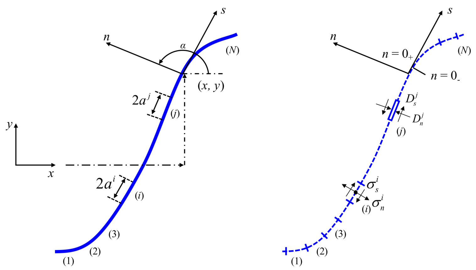
2.1. Displacement Discontinuity Method

The displacement discontinuity method is an efficient and economical numerical method which has been extensively used in fracture mechanics. The two-dimensional displacement discontinuity method was introduced by Crouch [70]. It is based on the analytical solution to the problem of a constant dislocation over a finite line segment in an elastic body.

Through discretizing an arbitrarily curved fracture with N elements, as shown in Figure 1, the displacements and stresses along the fracture can be easily formulated:

$$\begin{array}{l}{\sigma }_s^i={\displaystyle \sum _{j=1}^N{A}_{ss}\left(i,j\right)D_s^j}+{\displaystyle \sum _{j=1}^N{A}_{sn}\left(i,j\right)D_n^j}\hfill \\ {\sigma }_n^i={\displaystyle \sum _{j=1}^N{A}_{ns}\left(i,j\right)D_s^j}+{\displaystyle \sum _{j=1}^N{A}_{nn}\left(i,j\right)D_n^j}\hfill \\ u_s^i={\displaystyle \sum _{j=1}^N{B}_{ss}\left(i,j\right)D_s^j}+{\displaystyle \sum _{j=1}^N{B}_{sn}\left(i,j\right)D_n^j}\hfill \\ u_n^i={\displaystyle \sum _{j=1}^N{B}_{ns}\left(i,j\right)D_s^j}+{\displaystyle \sum _{j=1}^N{B}_{nn}\left(i,j\right)D_n^j}\hfill \end{array}\mathrm{for}i,j=1\mathrm{to}N$$

(1)

where ${\sigma }_s^i$ and ${\sigma }_n^i$ are the shear and normal components of stress at the midpoint of the i-th element; $u_s^i$ and $u_n^i$ are the shear and normal displacements of the i-th element; $D_s^j$ and $D_n^j$ are the components of discontinuity in the s and n directions of the j-th element, as shown in Figure 1b, each element has two surfaces, one is on the positive side of n (n = 0₊) and another is on the negative side, denoted n = 0₋. When crossing from one side of the line element to the other, the displacements undergo a constant change in value. Therefore, the displacement discontinuities $D_s^j$ and $D_n^j$ can be written as: $D_s^j=u_s^j\left(s,0_{-}\right)-u_s^j\left(s,0_{+}\right),D_n^j=u_n^j\left(s,0_{-}\right)-u_n^j\left(s,0_{+}\right)$.$A_{ss}\left(i,j\right)$, etc., are the boundary influence coefficients for the stresses, while $B_{ns}\left(i,j\right)$, etc., are the boundary influence coefficients of the displacements.

Given the prescribed stress or displacement boundary conditions, Equation (1) is a system of equations with 2N unknown displacement discontinuity components. These equations can be solved by standard methods, either direct or indirect. In this study, an iterative method called the “method of successive over-relaxation” is used. Details are provided in Appendix A.

2.2. Fracture Initiation and Propagation

The maximum circumferential stress criterion is used to predict the fracture initiation angle and propagation path [71]. This failure criterion states that a fracture will start its propagation when the stress intensities satisfy the following inequality:

$$\cos \frac{\theta }{2}\left[K_{\mathrm{I}}{\cos }^2\frac{\theta }{2}-\frac{3}{2}{K}_{\mathrm{II}}\sin \theta \right]\ge K_{\mathrm{I}C}$$

(2)

where K_I and K_II are the stress intensity factors; K_IC is fracture toughness; θ is the fracture initiation angle and satisfy the following equation:

$$K_{\mathrm{I}}\sin \theta +K_{\mathrm{II}}\left(3\cos \theta -1\right)=0$$

(3)

With DDM, the stress intensity factors K_I and K_II can be directly calculated by using the fracture tip element displacement discontinuities (DDs):

$$\begin{array}{l}{K}_{\mathrm{I}}=C\left(\frac{\sqrt{\pi }E}{4\left(1-v^2\right)\sqrt{\mathrm{\Delta }a}}\right)D_n\\ K_{\mathrm{II}}=C\left(\frac{\sqrt{\pi }E}{4\left(1-v^2\right)\sqrt{\mathrm{\Delta }a}}\right)D_s\end{array}$$

(4)

where E is the modulus of elasticity; v is the Poisson’s ratio; Δa is the length of the tip element; D_n and D_s are the displacement discontinuities of the tip element; C is an empirical correction coefficient, C = 0.806 proposed by Olson [72] is used in this paper.

The fracture propagation path is obtained by adding a new element to the end of the fracture. The length of the newly initiated element is equal to the original fracture tip element. The calculation accuracy can be improved by shortening the element length.

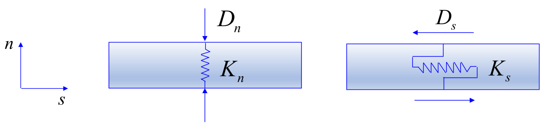
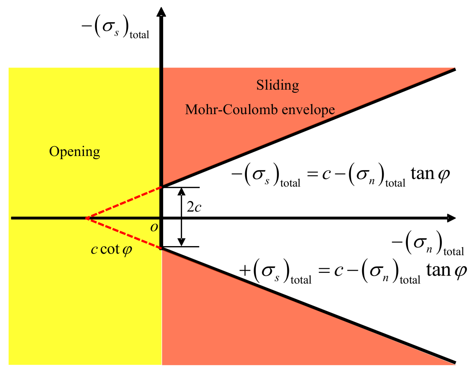
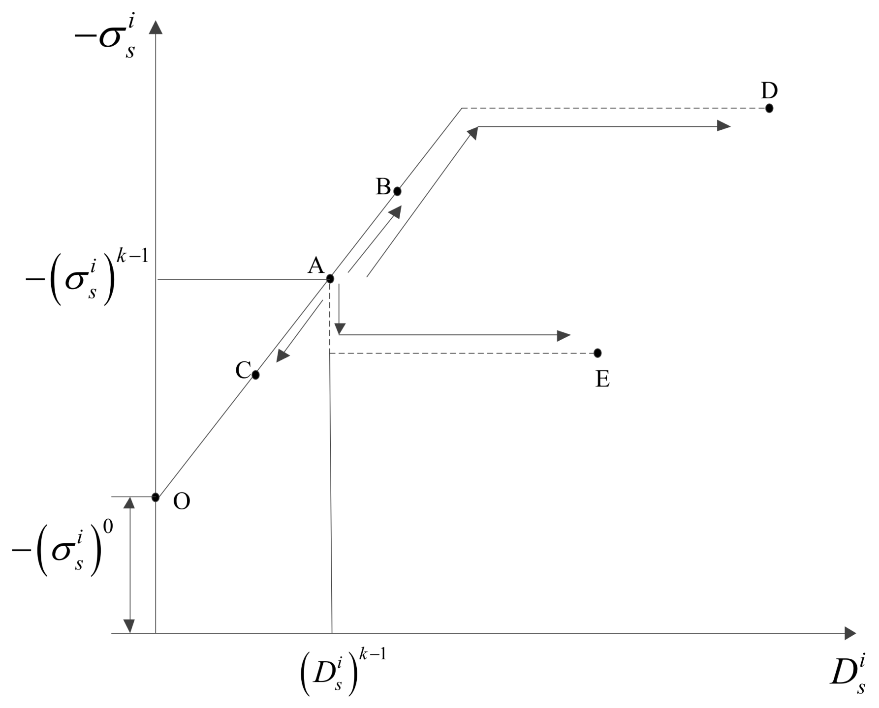
2.3. Mohr-Coulomb Joint Element

A special element, referred to as the joint element is used to model the effects of geologic discontinuities, i.e., faults and natural fractures in the rock mass. Unlike the constant displacement discontinuity element, a joint element can be visualized as an elemental displacement discontinuity whose opposite surface are connected by a spring, as shown in Figure 2.

A joint element with two degrees of freedom, the stress-strain relations can be easily written as:

$$\begin{array}{l}{\sigma }_n=-K_n{D}_n\hfill \\ {\sigma }_s=-K_s{D}_s\hfill \end{array}$$

(5)

where K_n and K_s are the normal and stress stiffnesses of the springs, which are chosen to representative of the properties of the fracture filling material.

If a closed natural fracture is divided by N joint element, the equations between tractions and the DDs can be written as:

$$\begin{array}{l}0=K_{\mathrm{s}}^i{D}_s^i+{\displaystyle \sum _{j=1}^N{A}_{ss}\left(i,j\right)D_s^j+{\displaystyle \sum _{j=1}^N{A}_{sn}\left(i,j\right)D_n^j}}\hfill \\ 0=K_n^i{D}_n^i+{\displaystyle \sum _{j=1}^N{A}_{ns}\left(i,j\right)D_s^j+{\displaystyle \sum _{j=1}^N{A}_{nn}\left(i,j\right)D_n^j}}\hfill \end{array}\mathrm{for}i=1\mathrm{to}N$$

(6)

where $D_n^i$ and $D_s^i$ are the total deformations of the i-th joint element, which usually be represented as the sum of the initial displacements (($D_n^i$)₀ and ($D_s^i$)₀) and the induced displacements ($D_n^{’i}$ and $D_s^{’i}$). In this study, the initial deformations of the natural fracture were not considered, so the total deformations of the joint element is equal to the induced displacements.

In reality, there must be a constraint on the maximum shear stress that can be developed across the joint. Such a constraint is given by the Mohr-Coulomb condition, as shown in Figure 3:

$$\left|{\left({\sigma }_s^i\right)}_{\mathrm{total}}\right|\le c^i+{\left(-{\sigma }_n^i\right)}_{\mathrm{total}}\tan {\phi }^i$$

(7)

where cⁱ and φⁱ are the cohesive and angle of friction of the joint-filling material.

When a joint element satisfies the constraint expressed by Equation (7), it will be called a Mohr-Coulomb element. The inelastic deformation of the natural fracture can be accurately simulated by using this special element. It is required that the element be allowed to undergo a certain amount of inelastic deformation or permanent slip, when the total shear stress on the joint element exceeds the total yield stress. Suppose that loading increment k − 1 has been completed, and no inelastic deformation occurred during this or any previous increment, the total shear stress ${\left({\sigma }_s^i\right)}_{\mathrm{total}}^{k-1}$ and shear displacement discontinuity ${\left(D_s^i\right)}^{k-1}$ will lie at some point A (see Figure 4). At the next loading increment, the i-th element may load or unload elastically (points B and C), or it may fail in accordance with Equation (1) (points D and E).

If the magnitude of the shear stress exceed the value of the yield stress σ_s,yield from Equation (7), the total shear stress must equal the yield stress, and so the corresponding equations can be modified as follows:

$$\begin{array}{l}\pm {\sigma }_{s,yield}^i-{\left({\sigma }_s^i\right)}_0={\displaystyle \sum _{j=1}^N{A}_{ss}\left(i,j\right)D_s^j}+{\displaystyle \sum _{j=1}^N{A}_{sn}\left(i,j\right)D_n^j}\hfill \\ 0=K_n{D}_n^i+{\displaystyle \sum _{j=1}^N{A}_{ns}\left(i,j\right)D_s^j+{\displaystyle \sum _{j=1}^N{A}_{nn}\left(i,j\right)D_n^j}}\hfill \end{array}\mathrm{for}i=1\mathrm{to}N$$

(8)

where ${\left({\sigma }_s^i\right)}_0$ is the initial shear stress; the sign selection of the yield stress is consistent with the total shear stress:

$$\mathrm{sign}\left({\sigma }_{s,yield}^i\right)=\mathrm{sign}\left({\left({\sigma }_s^i\right)}_{\mathrm{total}}\right)$$

(9)

In the above discussion, we have tacitly assumed that the normal stress across a joint element is compressive. According the Mohr-Coulomb condition (Equation (7)), if the stress greater than $c\cot \phi$ as shown in Figure 3, another failure model is possible, namely joint separation or crack open. In this study, we assume that natural fractures cannot bear tensile forces. Therefore, if the normal stress on a joint element changes from compressive stress to tensile stress, an opened Mohr-Coulomb element is formed. For such an element, the boundary conditions are that the total normal and shear stresses are zero. In this case, a cracked Mohr-Coulomb element is equivalent to a constant displacement discontinuity element, so the following equations must be satisfied:

$$\begin{array}{l}-{\left({\sigma }_s^i\right)}_0={\displaystyle \sum _{j=1}^N{A}_{ss}\left(i,j\right)D_s^j}+{\displaystyle \sum _{j=1}^N{A}_{sn}\left(i,j\right)D_n^j}\hfill \\ -{\left({\sigma }_n^i\right)}_0={\displaystyle \sum _{j=1}^N{A}_{ns}\left(i,j\right)D_s^j+{\displaystyle \sum _{j=1}^N{A}_{nn}\left(i,j\right)D_n^j}}\hfill \end{array}\mathrm{for}i=1\mathrm{to}N$$

(10)

where ${\left({\sigma }_s^i\right)}_0$ and ${\left({\sigma }_n^i\right)}_0$ are the initial shear and normal stresses.

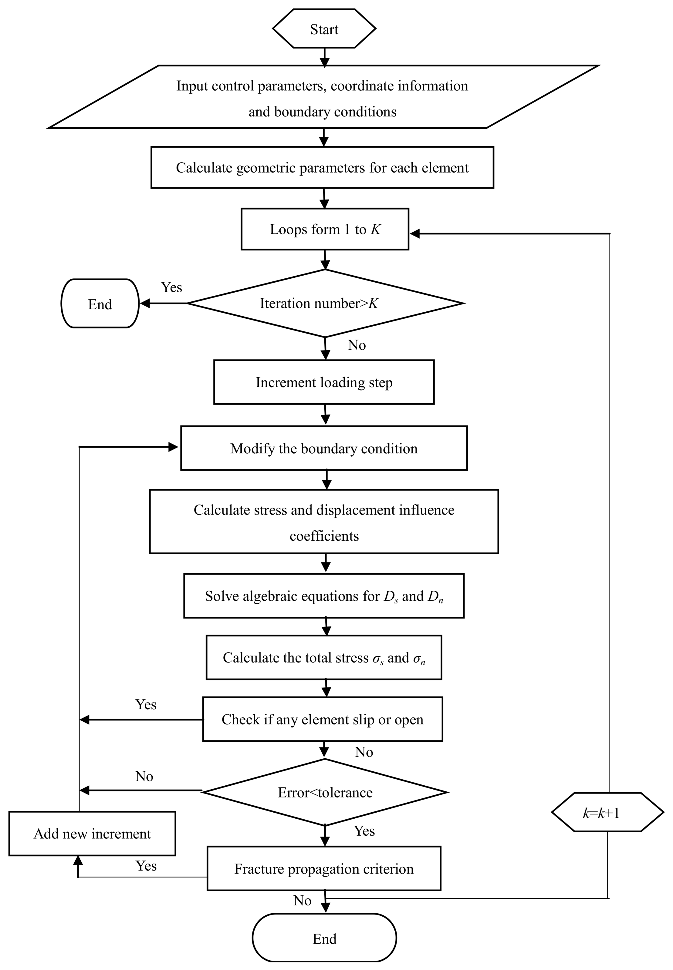
2.4. Numerical Procedure

The occurrence of slip along a joint is a nonlinear, path-dependent phenomenon, which must be modeled by an incremental process. In this paper, the final state is reached after K increments. The detailed iterative procedure is shown in Figure 5.

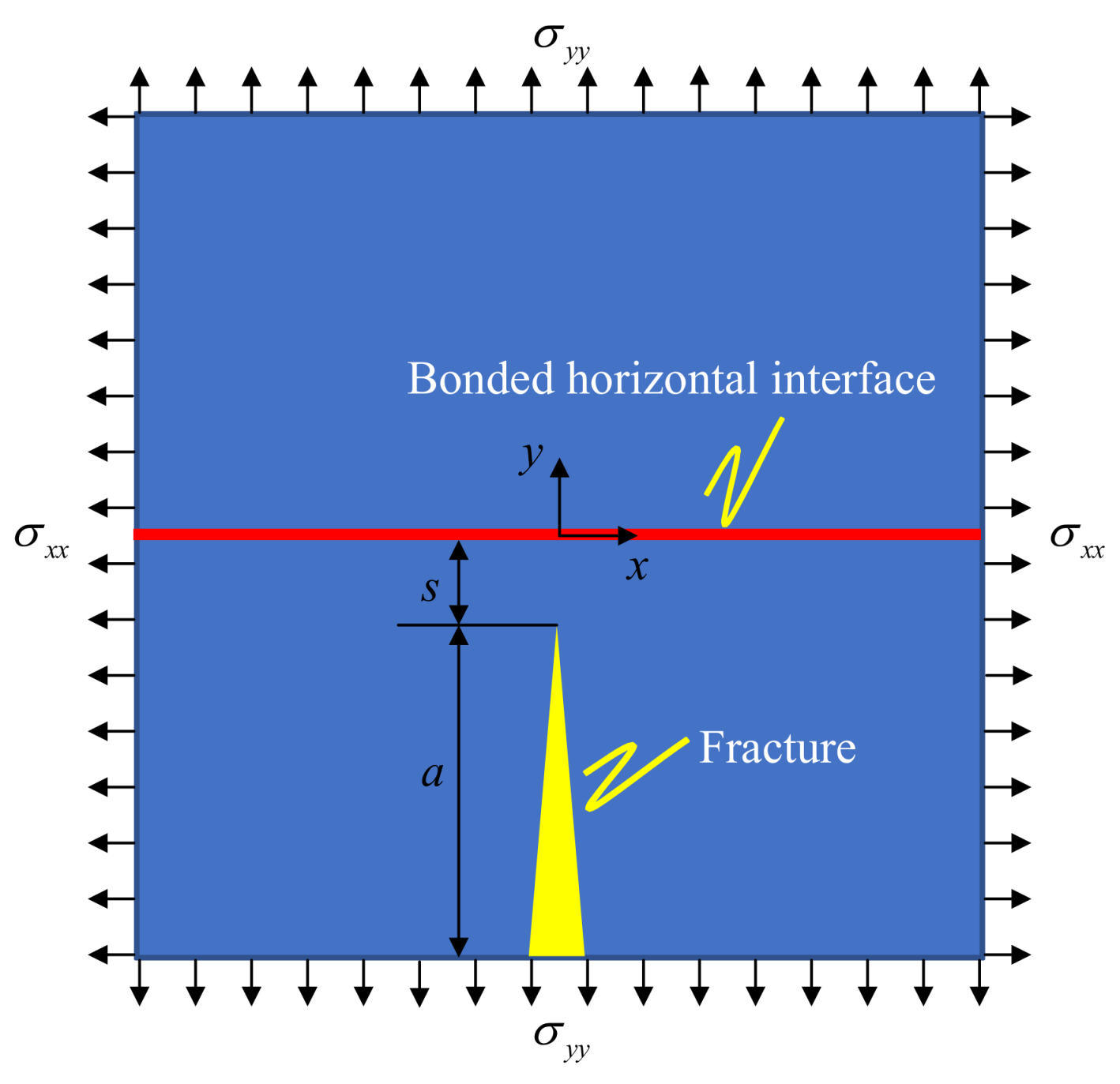
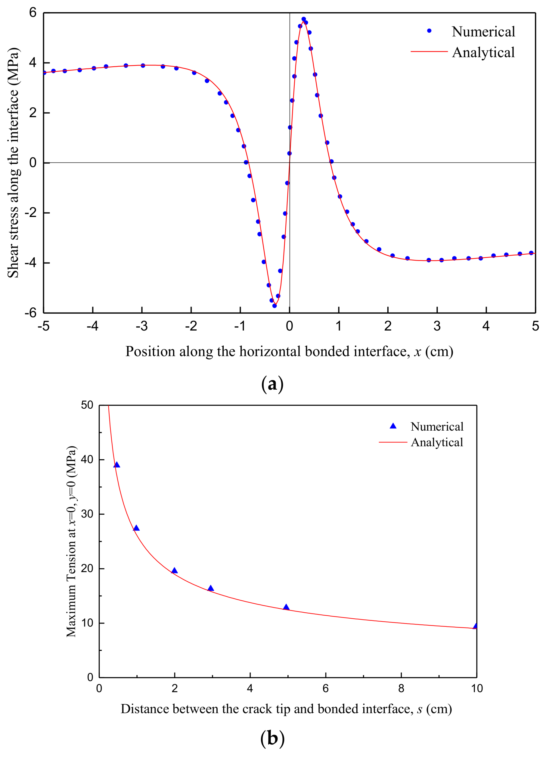
3. Model Verifications

The accuracy of the numerical model is validated by calculating the stress distribution along a bonded horizontal interface just ahead of a vertical opening fracture. The geometry of the model is shown in Figure 6. For simplicity, a uniform remote tensile (5 MPa) is used. The distance between the interface and the fracture tip is s; the vertical fracture length is 2a, which is 1-m-long; Young’s modulus is 20 GPa; Poisson’s ratio is 0.25. The analytical solutions can be easily derived from the Westergaard function (Appendix B).

As shown in Figure 7, a good agreement between the numerical results and analytical solutions is displayed. The small deviation may arise owing to the numerical discretization of the model and the use of the constant displacement discontinuity elements.

4. Case Studies

In this section, a series of numerical experiments have been performed to investigate the interaction between a hydraulic fracture and a pre-existing natural fracture. The geometry of the model is illustrated in Figure 8, a HF propagates along the direction of maximum horizontal stress and ultimately intersects an inclined NF. For simplicity, a fluid-uncoupled model is used herein owing to the desire specify a prescribed uniform pressure distribution along the HF. The parameters selected for these analyses are listed in

Table 1. The default value of the input parameters.

Parameter	Unit	Value
Initial length of natural fracture	m	2.0
Inclination of natural fracture	°	40
Cohesion of natural fracture	MPa	2.2
Friction angle of fracture	°	26.6
Normal stiffness of natural fracture	MPa/m	0.5 × 106
Shear stiffness of natural fracture	MPa/m	0.25 × 106
Initial Length of hydraulic fracture	m	2.0
Fluid pressure in the hydraulic fracture	MPa	−3.9
Initial gap between the fractures	m	0.1
Elasticity modulus	GPa	14
Poisson’s ratio	-	0.1
Maximum horizontal stress	MPa	−2.1
Minimum horizontal stress	MPa	−1.9

.

In the process of numerical calculation, the HF was discretized with 160 constant displacement discontinuity elements, each 1.25 cm wide. In addition, the NF was divided into 400 Mohr-Coulomb elements with an equal length of 0.5 cm.

To simplify the expression, some dimensionless parameters are introduced:

$$\begin{array}{c}\overline{x}=\frac{x}{L_{HF}},\overline{y}=\frac{y}{L_{HF}},\overline{\rho }=\frac{\rho }{L_{HF}}\\ {\overline{D}}_{s,n}=\frac{D_{s,n}}{L_{HF}}\frac{G}{\left(1-v\right){\sigma }_m},\prod =\frac{\left(p-{\sigma }_h\right)}{{\sigma }_m},\mathrm{\Delta }=\frac{{\sigma }_d}{{\sigma }_m}\end{array}$$

(11)

where $\overline{x}$ and $\overline{y}$ are the dimensionless coordinates; $\overline{\rho }$ are the normalized gap between the two fractures; ${\overline{D}}_{s,n}$ are the normalized displacement discontinuities; $\prod$ is the normalized net pressure; $\mathrm{\Delta }$ is the normalized horizontal stress difference; ${\sigma }_m$ and ${\sigma }_d$ are the average and difference of the horizontal stresses, respectively.

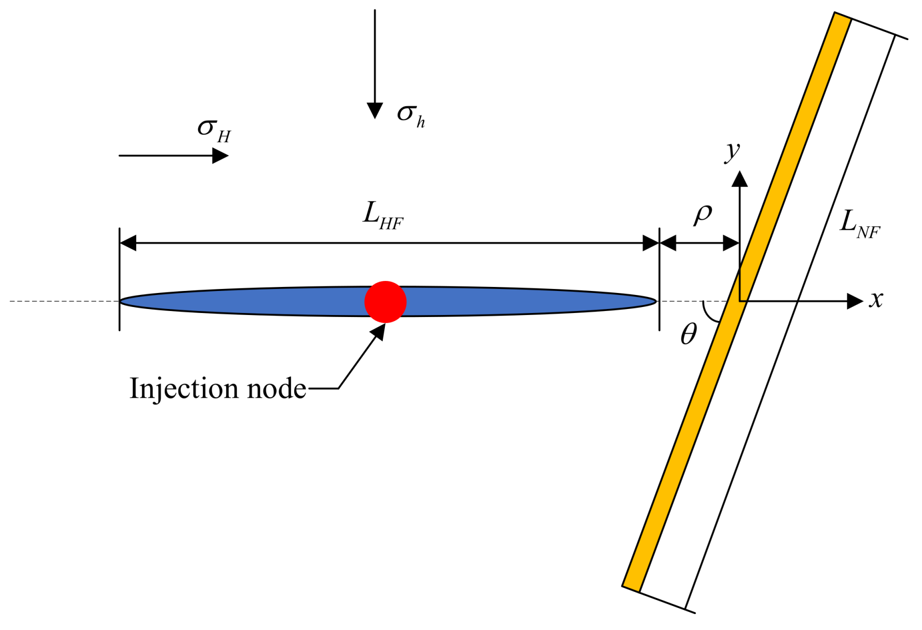
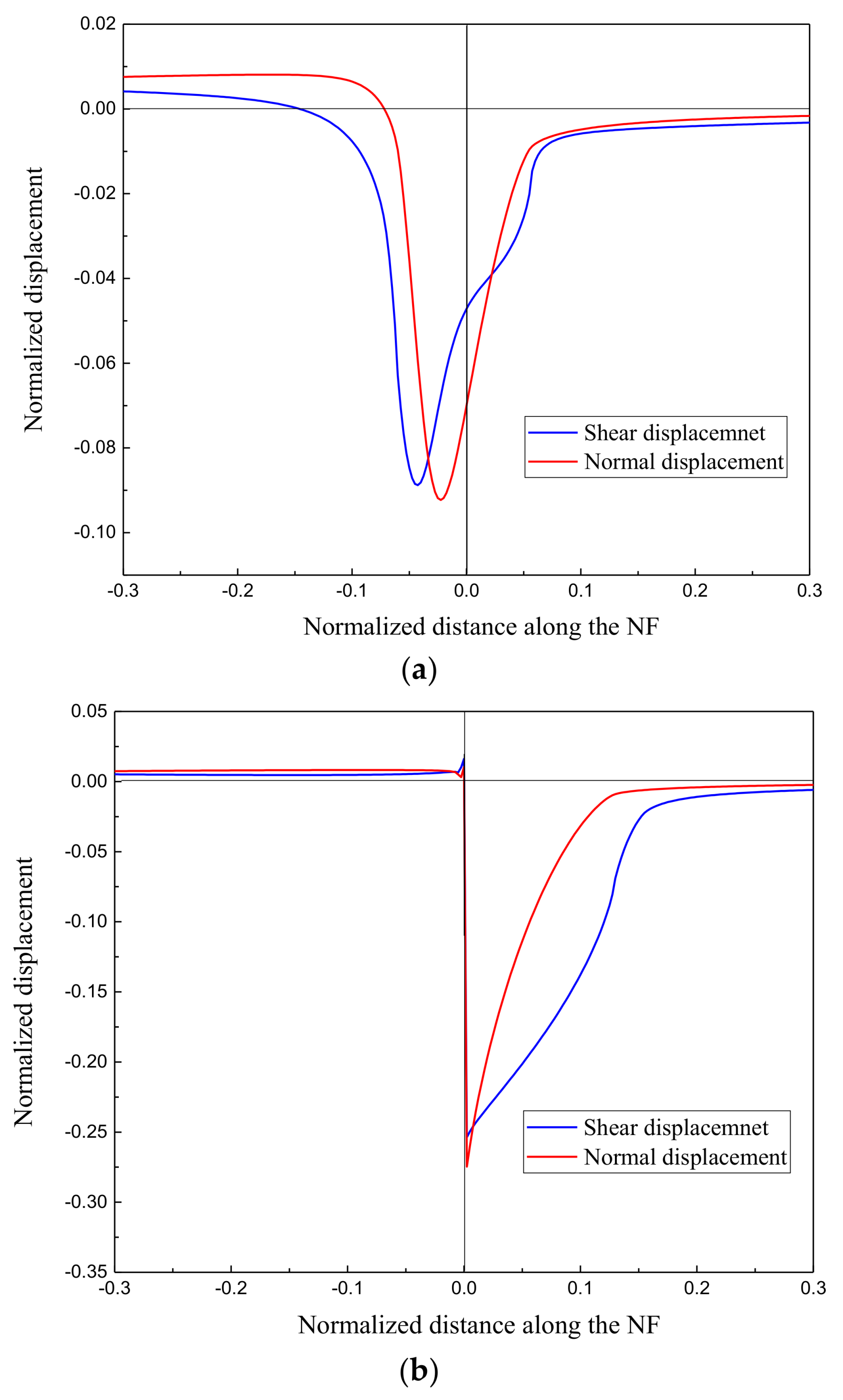
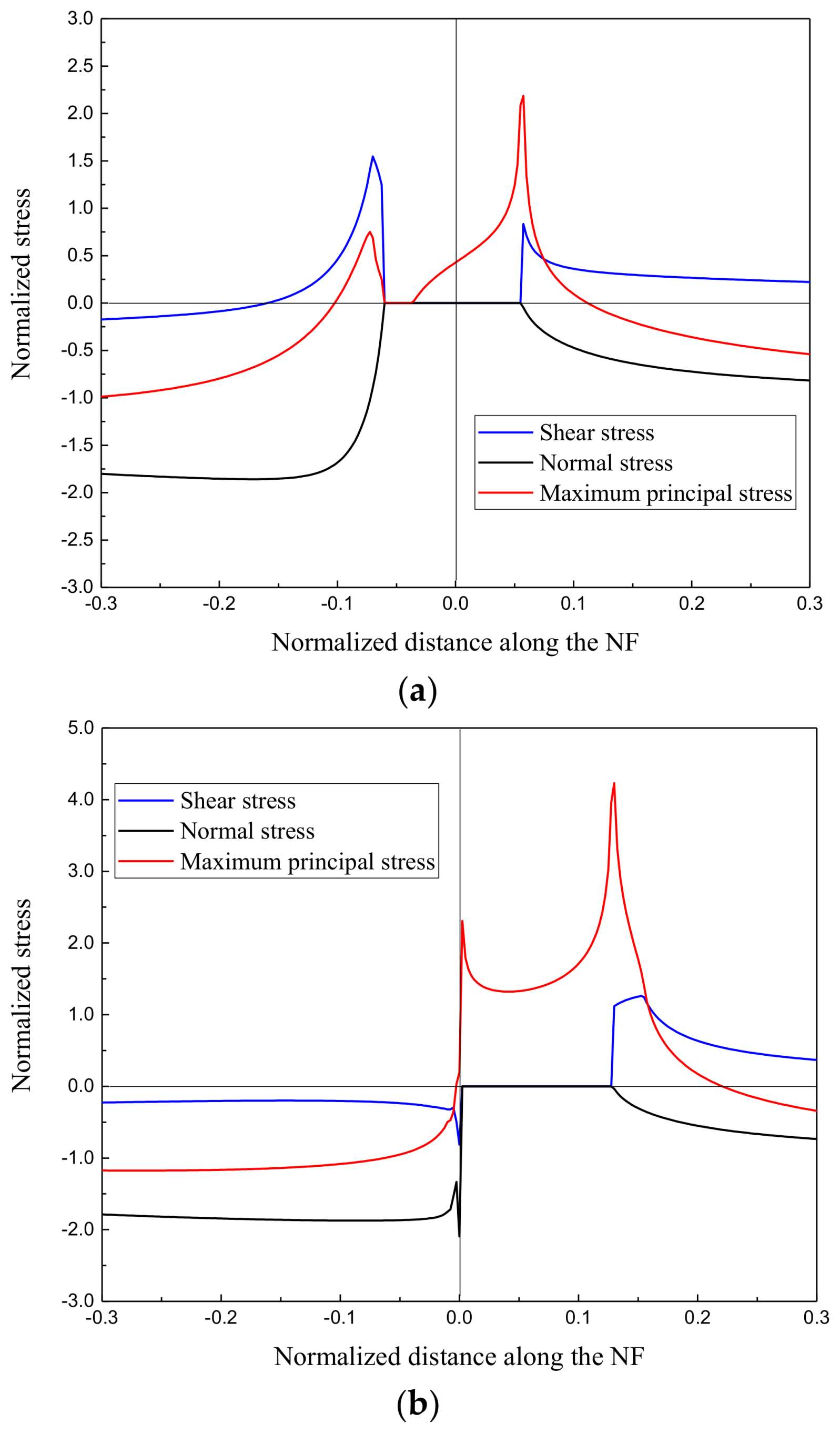
4.1. Displacements and Stresses along the Natural Fracture (NF)

The normalized shear and normal displacements along the NF with different fractures gap are shown in Figure 9. The results clearly indicated that the NF has been activated before intersecting with the HF, and the magnitudes of the displacements rapidly increase as the fractures gap decrease. In this case, the peak of normalized normal displacement is −0.27 when the fractures coalesce, which is three times bigger than that of the default fractures gap.

The normalized stresses along the NF are shown in Figure 10. From this figure, we can see that near the center of the NF, there is an opening zone where the shear and normal stresses are equal to zero, and the maximum principal stresses are located at the end of this zone. Meanwhile, the maximum principal stress has two different peak points, and the bigger one is located at the positive side of the NF, so secondary tensile cracks are more likely appear at this location. This result can be confirmed by the field test of Jeffrey [73].

Then, we analyse the distribution of the normalized maximum principal stress along the NF with different fractures gaps. As shown in Figure 11, we can see that with a decreasing fracture gap, the maximum principal stress increases dramatically, and the location of the peak is farther from the junction. Note that the induced maximum principal stress along the opposite side of the NF may exceed the tensile strength of the rock mass before the fracture coalescence.

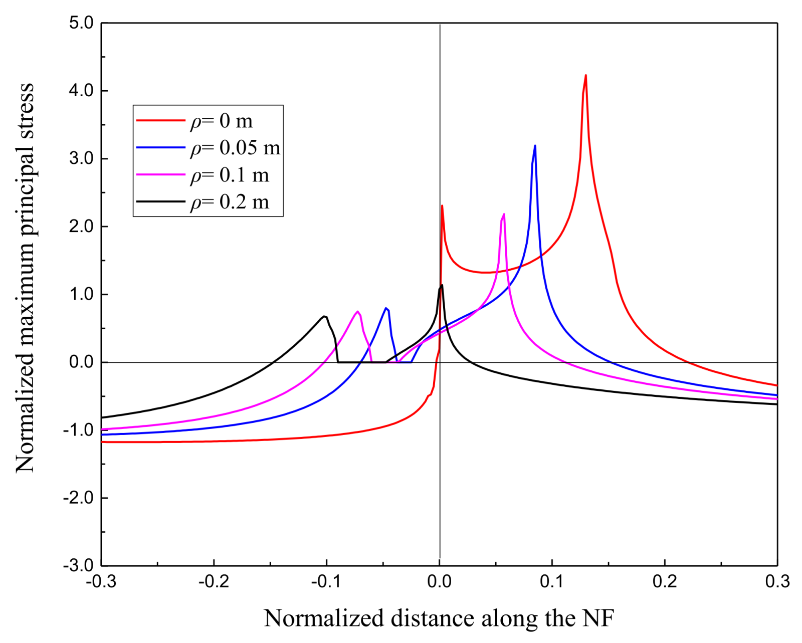
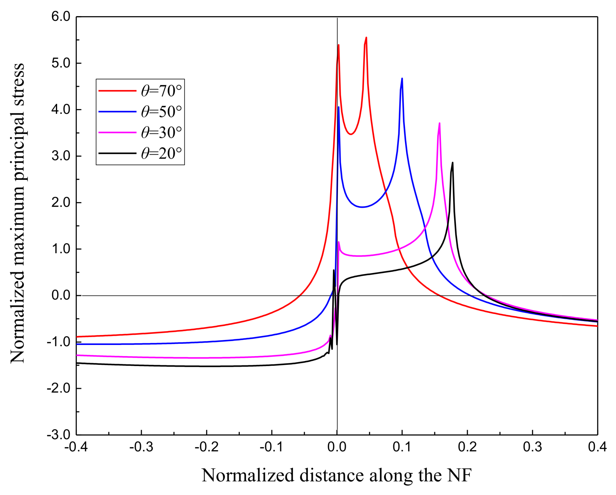
4.2. Parametric Study of Stress Distribution and Unstable Tensile Zone along the NF

Firstly, the natural fracture inclination is considered. As plotted in Figure 12 and Figure 13, we can see that NF slope angle has a significant impact on the stress distribution along the NF. With the increasing of the NF inclination, the magnitude of the maximum principal stress rapidly increases, but the peak value location is farther from the central of the NF. It means that the HF is prone to directly cross the high angle natural fracture.

Secondly, we focused our attention to HF net pressure Π and horizontal stress difference $\mathrm{\Delta }$. As shown in Figure 14, we can see that the offset of the maximum principal stress peak increases proportionally to the HF net pressure. It means that we can increase the fracture complexity by increasing the HF net pressure. However, the horizontal stress difference may have a negative effect on the fracture complexity. In this case, the offset of the maximum principal stress peak in a nonuniform in-situ stress field is smaller than that under a uniform stress.

Finally, the cemented strength of NF is being considered. The Mohr diagrams for the entire set of elements along the NF are depicted in Figure 15. The two inclined straight lines in each diagram represent the yield condition and are usually called Mohr-Coulomb envelope lines. The bracketed numbers refer to the element numbers. From this figure, it can be observed that for a moderate strength NF, the shear and tensile damages occur simultaneously. In this case, the elements (No. 201–252) in the range of 0.0 m < y < 0.26 m open, while the elements (No. 253–262) in the range of 0.26 m < y < 0.31 m undergo sliding. However, for a weak strength NF, only shear failure occurs. The elements (No. 202–365) in the range of 0.0 m < y < 0.82 m undergo sliding, which means that the HF is more likely to turn toward the NF direction.

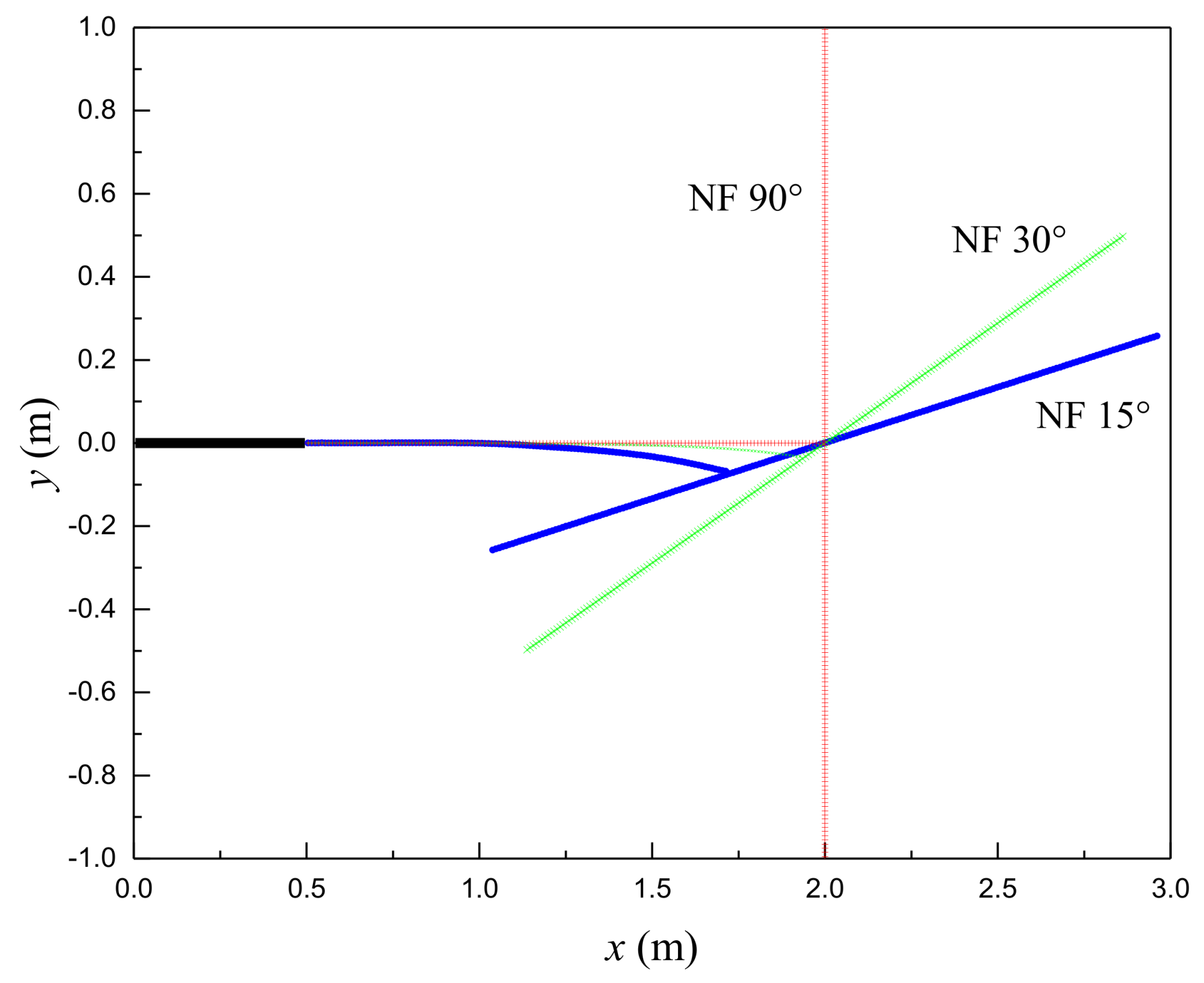
4.3. Effects of Natural Fracture on the Hydraulic Fracture (HF) Propagation Path

The accurate prediction and monitoring of hydraulic fracturing propagation pathways is very important for reservoir stimulation practice. Therefore, the flowing numerical simulations are conducted to investigate the influence of NF on the HF trajectories. The main parameters required for the model are derived from [44]. One issue that needs to be especially pointed out is that the initial deformation of the natural fracture is also not considered in this case. The HF trajectories for different NF inclination angles are depicted in Figure 16. From this figure, we can see that the NF inclination angle has an important effect on the shape of the HF propagation path. When the NF inclination is 90°, the HF extends parallel to the x-axis until it crosses the NF. However, as the slope angle decreases, the left side of the NF (i.e., y < 0) is closer to the HF surface, and the direction of the maximum principal stress in front of the NF will change. Thus, the HF is more prone to deviate from its original propagation path and reorientation near the NF.

5. Experimental Investigation

For better understanding of the mechanics of how the NFs affect the HF initiation and propagation and validation of the numerical model results, a series of laboratory stimulated experiments were carried out on the Longmaxi shale outcrops collected from Sichuan Base, China.

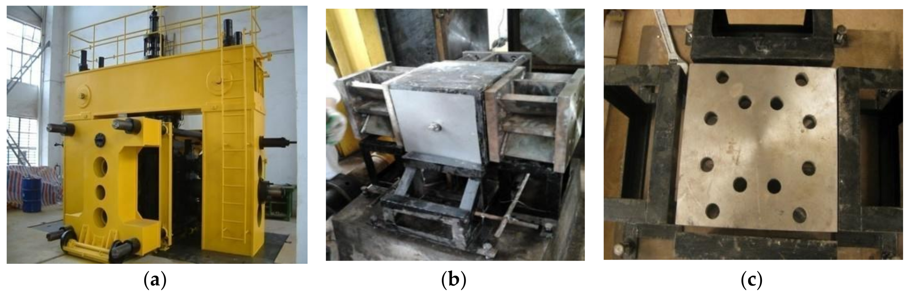
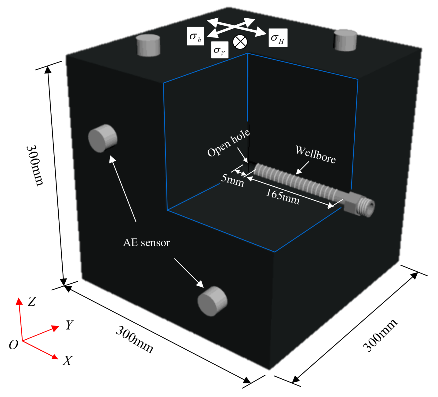
5.1. Experimental Setup and Sample Preparation

The apparatus used in this study was a large-scale, true tri-axial hydraulic fracturing test system (as shown in Figure 17), capable of subjecting an 800 × 800 × 800 mm block to magnitudes of confining stress up to 30 MPa. The hydraulic fluid injection rate and pressure were precisely controlled by an individual hydraulic pump pressure servo control system. The maximum hydraulic fluid injection pressure could reach values up to 100 MPa. Apart from these variables, an acoustic emission monitoring system (that contained eight probes, operated within a frequency range of 15–75 kHz, with resonant frequencies of 40 kHz, and a minimum noise threshold of 18 dB), was used to detect the acoustic signal during fracture initiation and propagation.

Two cube samples of 300 mm × 300 mm × 300 mm were prepared for these experiments. Each block had a simulated wellbore (diameter: 24 mm; length: 170 mm) in its center, with the axis of the borehole parallel to the minimum horizontal stress. Two slotted steel pipes (diameter: 20 mm; pipe thickness: 2.5 mm) were then cemented with epoxy onto the simulated wellbore, leaving a 5 mm open-hole section at the lower side of the wellbore. The direction of wellbore and in-situ stresses are shown in Figure 18. For each experiment, water with red fluorescent dye was injected into the wellbore. The experimental scheme is shown in

Table 2. Experimental scheme and parameters.

Specimen Number	Simulated Well Type	Liquid Type	σv (MPa)	σH (MPa)	σh (MPa)	Flow Rate (ML/s)
Y-7-1	horizontal well	fresh water	20.00	19.51	16.98	0.5
Y-7-3						1.0

.

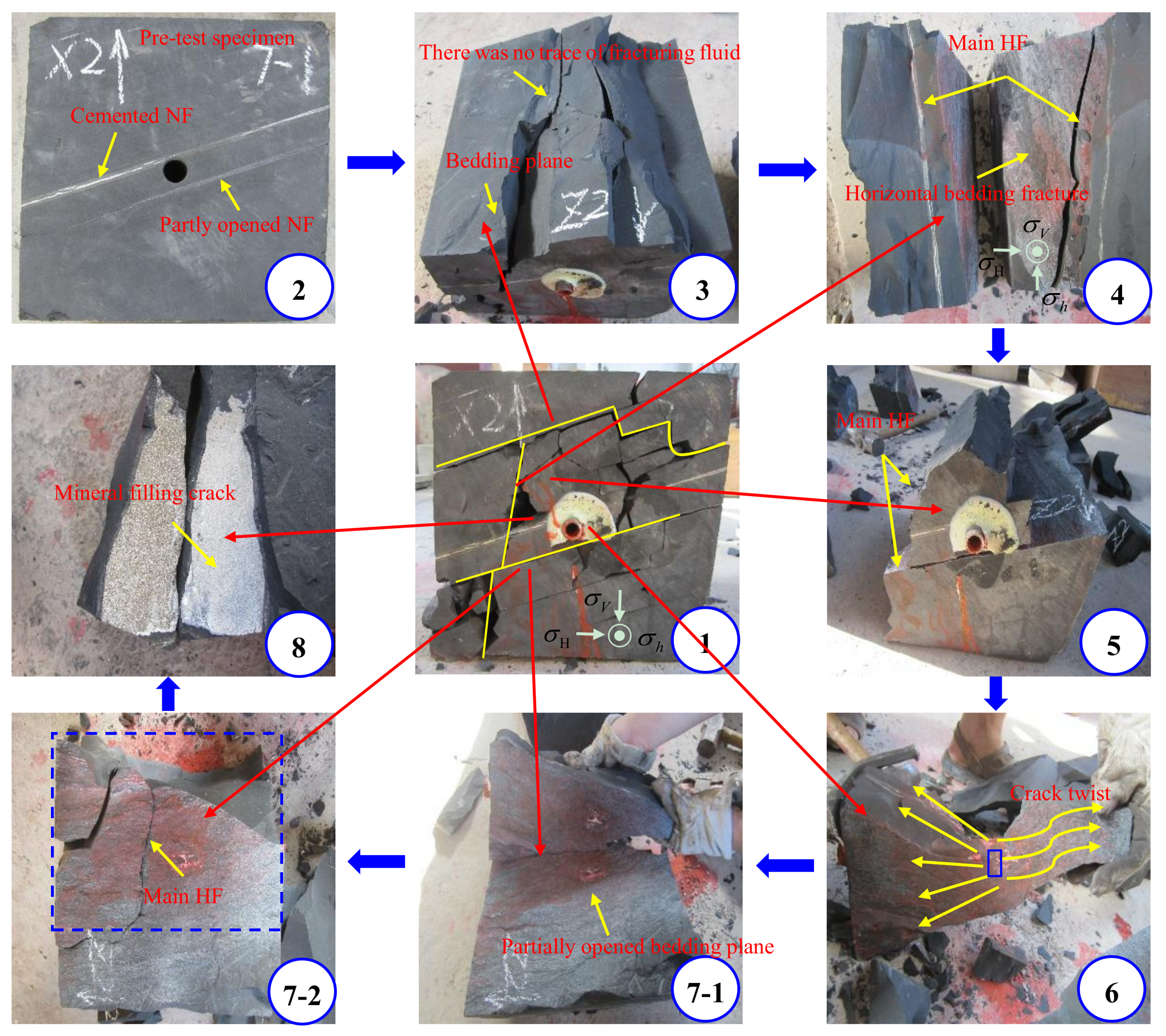
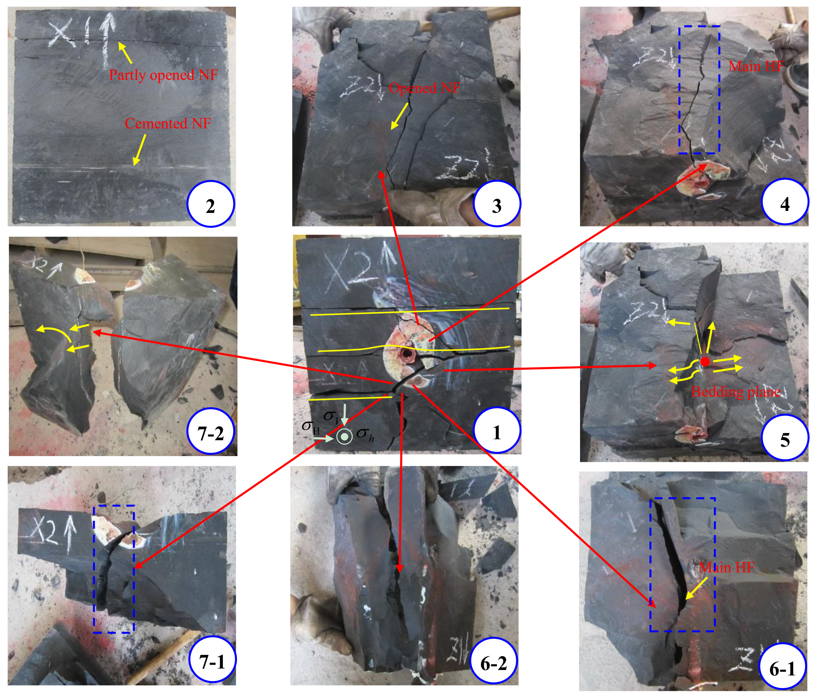
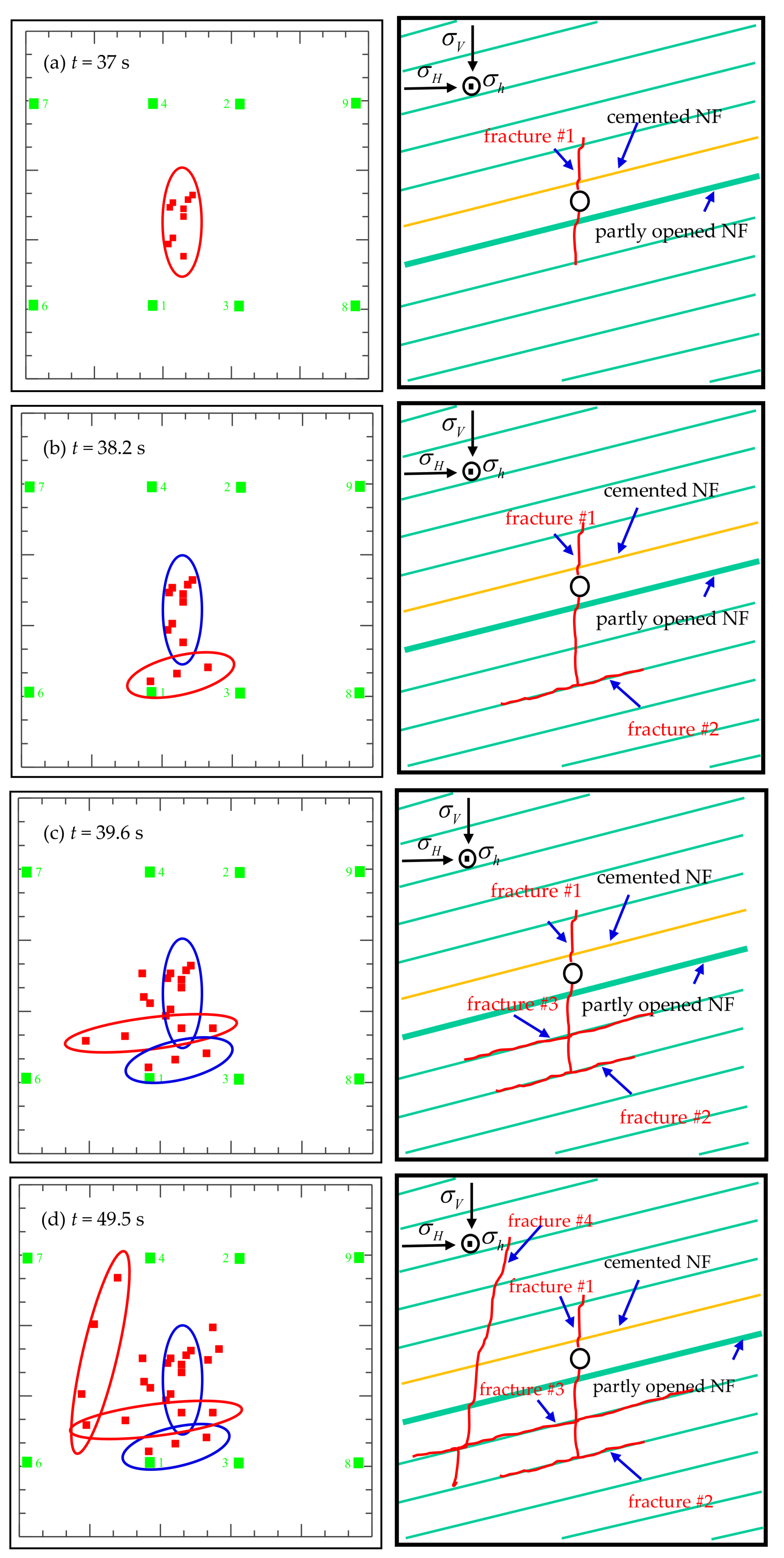
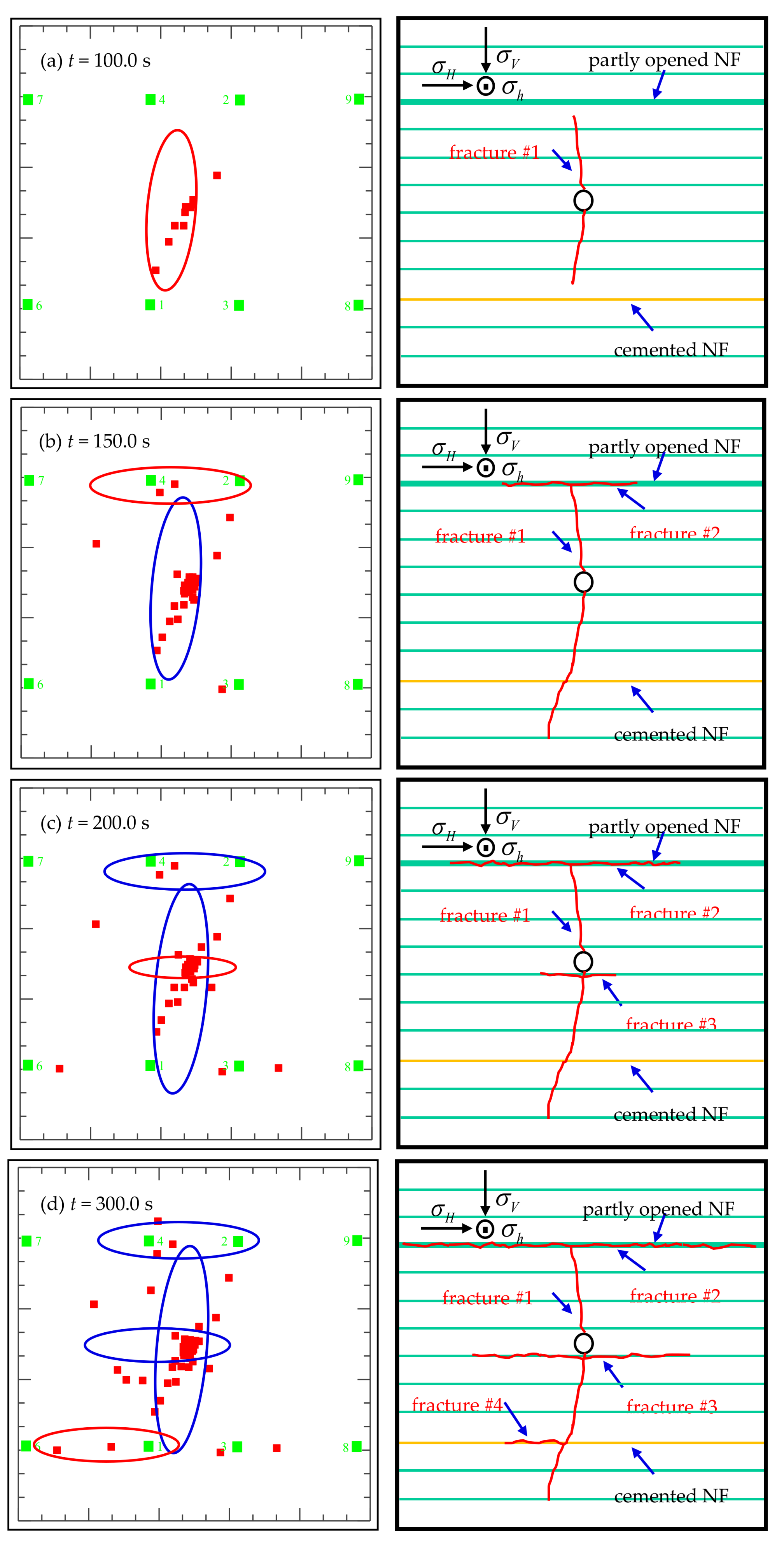
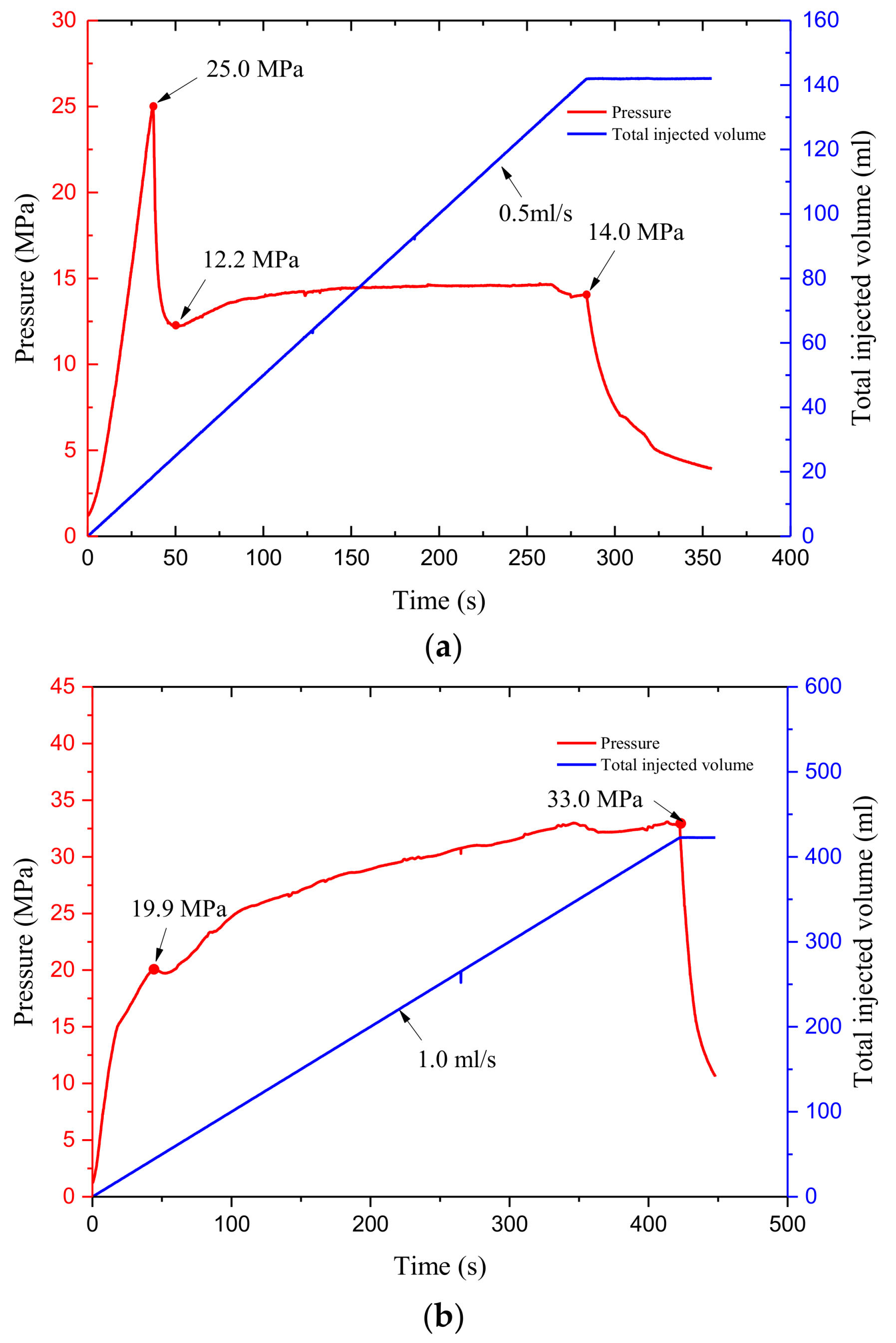
5.2. Experimental Results and Analyses

Photographs of the cube after the fracturing tests are shown in Figure 19 and Figure 20. It is found that the geometry of the shale hydraulic fracture is more complex, which is different from the traditionally bi-winged, planar fracture. The morphology of the HF is strongly influenced by the opened NFs and sedimentary beddings.

The crack initiation and evolution can also be analyzed by the acoustic emission (AE) detection results during experiments. One red dot is defined as an AE event. For specimen Y-7-1 (shown in Figure 21), the HF firstly began to propagate along the overburden stress, lately extended to an inclined pre-existing natural fracture (fracture #1). Shortly, some acoustic emission events were gradually appeared along the natural fracture (fracture #2). These AE events were most probably generated by shear slippage along the NF surface since fluid that leaked off increased the pressure and reduced the cemented strength. As time elapsed, the fluid pressure was sufficient to create a new secondary fracture at the weak location on the surface with the natural fracture. Thus, a step-like fracture with an obvious lateral offset was formed in the vertical direction (fracture #3). At the same time, some additional secondary fractures near the crack junction were also formed by the higher fluid pressure (fracture #4). Finally, the hydraulic fracture was arrested by a partially opened bedding fracture at the upper side and extended to the outer surface of the specimen at the lower left corner.

For another specimen, labeled Y-7-3 (shown in Figure 22), the HF firstly propagated along the direction of the overburden stress (fracture #1), and thus turned into an opened bedding fracture (fracture #2). Soon afterwards, the partially opened bedding fracture near the wellbore was activated by the higher fluid pressure (fracture #3). As time elapsed, another pre-existing bedding fracture (fracture #4) was also activated by the main hydraulic fracture (fracture #1). Finally, a discrete fracture network was formed, but the complexity of the final fracture network was lower than that of specimen Y-7-1.

The variation curves of the pump pressure and total injected volume during the tests are shown in Figure 23. It can be observed that there is a significant difference between the pump pressure curves of the two model blocks. In test Y-7-1, a typical pump pressure curve was recorded, and an obvious fracture breakdown was indicated by a sharp decline of the pump pressure. However, for specimen Y-7-3, it was difficult to see obvious fracture breakdown characteristics from the pump pressure curve, and the pump pressure continued to rise until a stable hydraulic flow channel had been fully formed. This was because the hydraulic fractures were mainly propagating along the opened bedding fracture, and a higher fluid pressure was needed to overcome the overburden stress and stress shadow. In addition, the larger total injected volume and less AE events indicate that the specimen Y-7-3 was dominated by tensile failure and the sample Y-7-1 was mainly present in the form of shear failure.

Based on these experimental results, we found that the morphology of the shale hydraulic fracture was strongly influenced by the characteristics of the pre-existing natural fractures and sedimentary beddings. The density, orientation, and cemented strength of the pre-existing natural fractures are the three factors dominating the formation of complex fracture networks. The hydraulic fractures are either diverted or arrested by the NF. The experiment results are in good agreement with the numerical results.

6. Conclusions

Based on these numerical and experimental analyses, the following conclusions can be proposed:

(1)

The hydraulic fracture morphology of shale was strongly influenced by the characteristics of its natural fractures. The NF density, orientation, and cemented strength, are three main factors dominating the formation of complex fracture networks.

(2)

The cemented strength of the NF caused a noticeable nonlinear behavior for this problem. For an NF with a low strength, only shear failure occurred, and the HF was more likely to terminate. However, for an NF with a moderate strength, the hybrid failure model (tensile failure and shear failure co-existence, and conversion) may occur, and the HF is more inclined to step over at the contact.

(3)

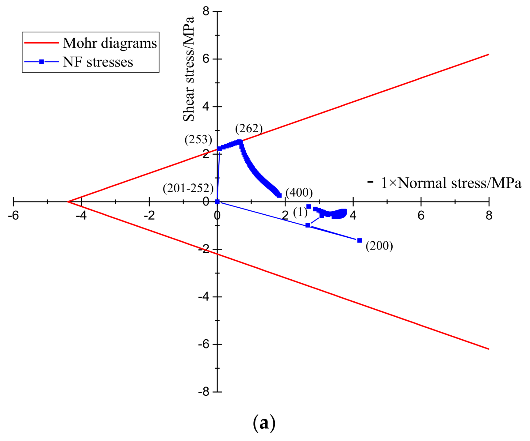
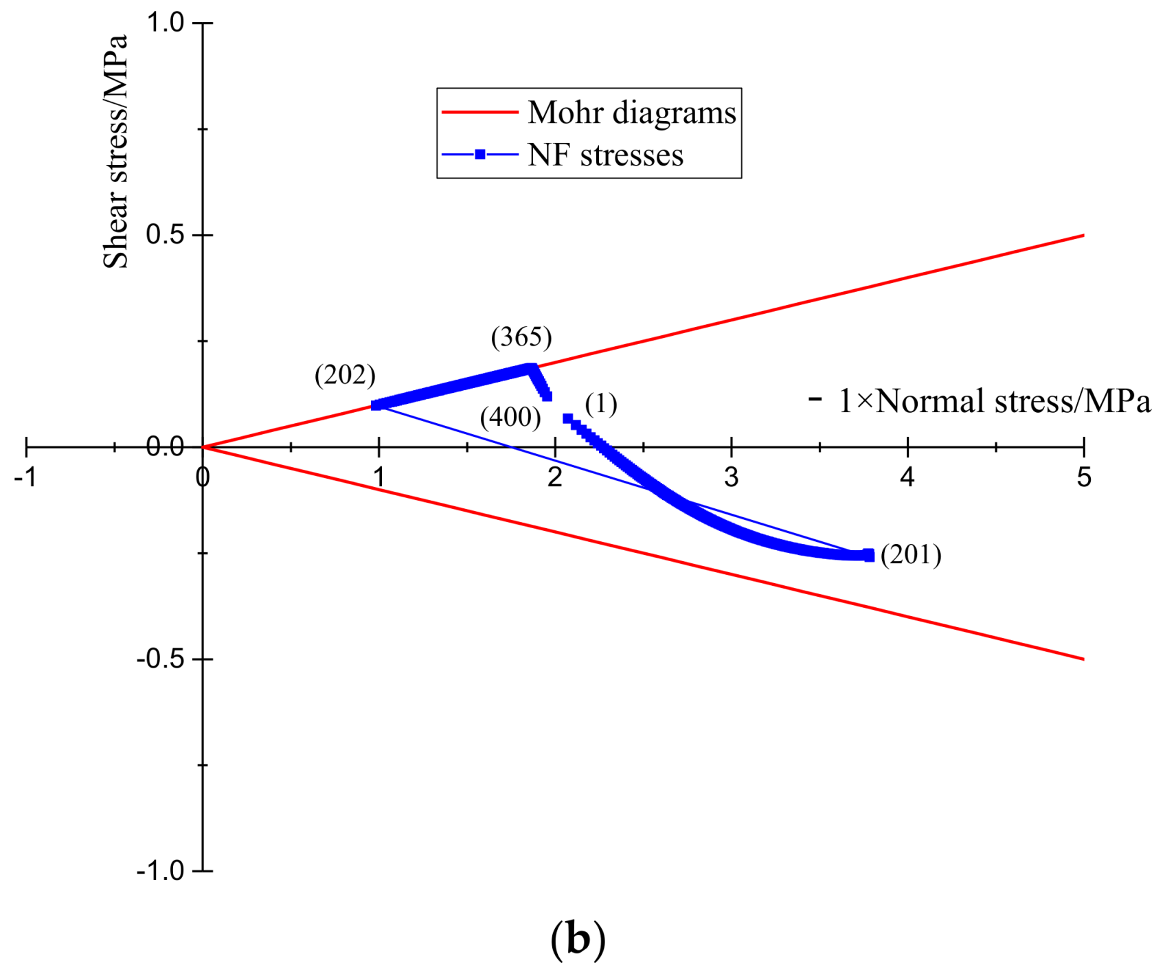
The displacements and stresses along the NF all changed in a highly dynamic manner. During the stage of approach of the HF to an NF, the HF tip could exert a remote compressional and shear stress on the NF interface, which could lead to the debonding of the natural fracture. Meanwhile, a maximum principal stress peak is generated at the end of the opening zone, where a new tensile crack is more likely to occur.

(4)

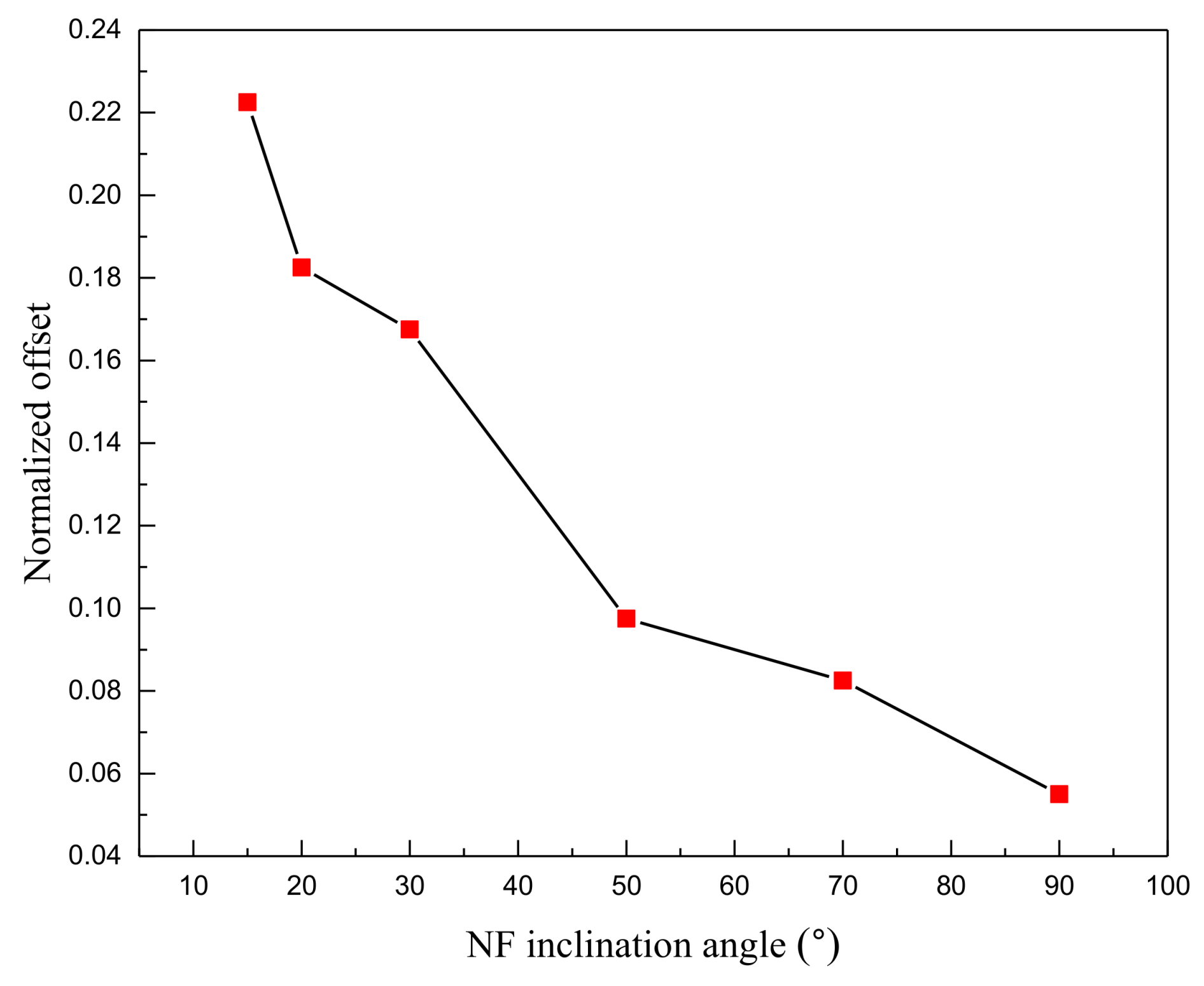
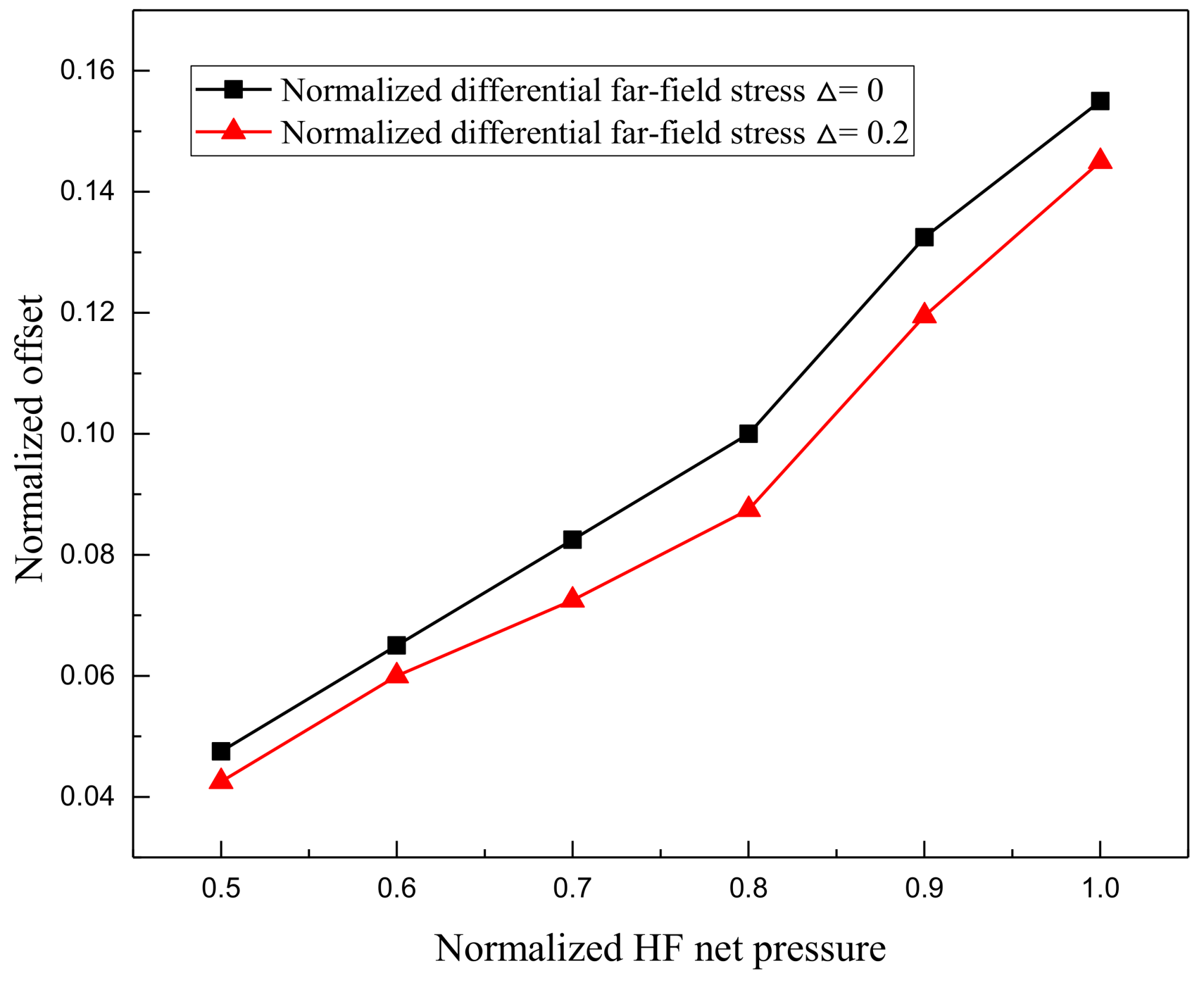
The location and value of the stress is the function of NF inclination angle, far-field differential stress as well as HF net pressure. For small approaching angles, the stress peak is located farther from the intersection point, so a step over (offset) fracture is more likely to occur. The same effect can be found by a higher HF net pressure, because the stress perturbation ahead the NF is proportional to the fluid pressure in the HF.

(5)

Meanwhile, the HF was found to be more prone to deviate from its original propagation path and reoriented near the NF because the deformation of the NF.

References

1. KERR, R.A. Natural Gas From Shale Bursts Onto the Scene. Science 2010, 328, 1624–1626. [Google Scholar] [CrossRef] [PubMed]
2. US Energy Information Administration. Annual Energy Outlook 2013; US Energy Information Administration: Washington, DC, USA, 2013; pp. 60–62. [Google Scholar]
3. US Energy Information Administration. Annual Energy Outlook 2011: With Projections to 2035; Government Printing Office: Washington, DC, USA, 2011.
4. Shen, W.; Li, X.; Xu, Y.; Sun, Y.; Huang, W. Gas flow behavior of nanoscale pores in shale gas reservoirs. Energies 2017, 10, 751. [Google Scholar] [CrossRef]
5. Gale, J.F.; Reed, R.M.; Holder, J. Natural fractures in the Barnett Shale and their importance for hydraulic fracture treatments. AAPG Bull. 2007, 91, 603–622. [Google Scholar] [CrossRef]
6. Daniels, J.L.; Waters, G.A.; Le Calvez, J.H.; Bentley, D.; Lassek, J.T. Contacting more of the Barnett Shale through an Integration of Real-Time Microseismic Monitoring, Petrophysics, and Hydraulic Fracture Design. In Proceedings of the SPE Annual Technical Conference and Exhibition, Anaheim, CA, USA, 11–14 November 2007. [Google Scholar]
7. Fisher, M.K.; Wright, C.; Davidson, B.; Goodwin, A.; Fielder, E.; Buckler, W.; Steinsberger, N. Integrating Fracture Mapping Technologies to Optimize Stimulations in the Barnett Shale. In Proceedings of the SPE Annual Technical Conference and Exhibition, San Antonio, TX, USA, 29 September–2 October 2002. [Google Scholar]
8. Maxwell, S.C.; Urbancic, T.; Steinsberger, N.; Zinno, R. Microseismic imaging of hydraulic fracture complexity in the Barnett shale. In Proceedings of the SPE Annual Technical Conference and Exhibition, San Antonio, TX, USA, 29 September–2 October 2002. [Google Scholar]
9. Lamont, N.; Jessen, F. The effects of existing fractures in rocks on the extension of hydraulic fractures. J. Pet. Technol. 1963, 15, 203–209. [Google Scholar] [CrossRef]
10. Daneshy, A.A. Hydraulic fracture propagation in the presence of planes of weakness. In Proceedings of the SPE European Spring Meeting, Amsterdam, The Netherlands, 29–30 May 1974. [Google Scholar]
11. Anderson, G.D. Effects of friction on hydraulic fracture growth near unbonded interfaces in rocks. Soc. Pet. Eng. J. 1981, 21, 21–29. [Google Scholar] [CrossRef]
12. Blanton, T.L. An experimental study of interaction between hydraulically induced and pre-existing fractures. In Proceedings of the SPE Unconventional Gas Recovery Symposium, Pittsburgh, PA, USA, 16–18 May 1982. [Google Scholar]
13. Warpinski, N.; Teufel, L. Influence of geologic discontinuities on hydraulic fracture propagation (includes associated papers 17011 and 17074). J. Pet. Technol. 1987, 39, 209–220. [Google Scholar] [CrossRef]
14. Beugelsdijk, L.; De Pater, C.; Sato, K. Experimental hydraulic fracture propagation in a multi-fractured medium. In Proceedings of the SPE Asia Pacific Conference on Integrated Modelling for Asset Management, Yokohama, Japan, 25–26 April 2000. [Google Scholar]
15. Zhou, J.; Chen, M.; Jin, Y.; Zhang, G.Q. Analysis of fracture propagation behavior and fracture geometry using a tri-axial fracturing system in naturally fractured reservoirs. Int. J. Rock Mech. Min. Sci. 2008, 45, 1143–1152. [Google Scholar] [CrossRef]
16. Olson, J.E.; Bahorich, B.; Holder, J. Examining hydraulic fracture: Natural fracture interaction in hydrostone block experiments. In Proceedings of the SPE Hydraulic Fracturing Technology Conference, The Woodlands, TX, USA, 6–8 February 2012. [Google Scholar]
17. Lee, H.P.; Olson, J.E.; Holder, J.; Gale, J.F.; Myers, R.D. The interaction of propagating opening mode fractures with preexisting discontinuities in shale. J. Geophys. Res. Solid Earth 2015, 120, 169–181. [Google Scholar] [CrossRef] [Green Version]
18. Alabbad, E.A.; Olson, J.E. Examining the Geomechanical Implicaitons of Pre-Existing Fractures and Simultaneous-Multi-Fracturing Completions on Hydraulic Fractures: Experimental Insights into Fracturing Unconventional Formations. In Proceedings of the SPE Annual Technical Conference and Exhibition, Dubai, UAE, 26–28 September 2016. [Google Scholar]
19. Blanton, T.L. Propagation of hydraulically and dynamically induced fractures in naturally fractured reservoirs. In Proceedings of the SPE Unconventional Gas Technology Symposium, Louisville, Kentucky, 8–21 May 1986. [Google Scholar]
20. Cheng, W.; Yan, J.; Mian, C.; Tong, X.; Zhang, Y.; Ce, D. A criterion for identifying hydraulic fractures crossing natural fractures in 3D space. Petr. Explor. Dev. 2014, 41, 371–376. [Google Scholar] [CrossRef]
21. Chuprakov, D.; Melchaeva, O.; Prioul, R. Hydraulic fracture propagation across a weak discontinuity controlled by fluid injection. In Proceedings of the Effective and Sustainable Hydraulic Fracturing, Brisbane, Australia, 20–22 May 2013. [Google Scholar]
22. Gu, H.; Weng, X. Criterion for fractures crossing frictional interfaces at non-orthogonal angles. In 44th US Rock Mechanics Symposium and 5th US-Canada Rock Mechanics Symposium; American Rock Mechanics Association: Salt Lake City, UT, USA, 2010. [Google Scholar]
23. Gu, H.; Weng, X.; Lund, J.B.; Mack, M.G.; Ganguly, U.; Suarez-Rivera, R. Hydraulic fracture crossing natural fracture at nonorthogonal angles: A criterion and its validation. SPE Prod. Oper. 2012, 27, 20–26. [Google Scholar] [CrossRef]
24. Potluri, N.; Zhu, D.; Hill, A.D. The effect of natural fractures on hydraulic fracture propagation. In Proceedings of the SPE European Formation Damage Conference, Sheveningen, The Netherlands, 25–27 May 2005. [Google Scholar]
25. Renshaw, C.; Pollard, D. An experimentally verified criterion for propagation across unbounded frictional interfaces in brittle, linear elastic materials. In International Journal of Rock Mechanics and Mining Sciences Geomechanics Abstracts; Elsevier: New York, NY, USA, 1995; pp. 237–249. [Google Scholar]
26. Sarmadivaleh, M.; Rasouli, V. Modified Reinshaw and Pollard criteria for a non-orthogonal cohesive natural interface intersected by an induced fracture. Rock Mech. Rock Eng. 2014, 47, 2107–2115. [Google Scholar] [CrossRef]
27. Yao, Y.; Wang, W.; Keer, L.M. An energy based analytical method to predict the influence of natural fractures on hydraulic fracture propagation. Eng. Fract. Mech. 2018, 189, 232–245. [Google Scholar] [CrossRef]
28. Bao, J.; Fathi, E.; Ameri, S. A coupled finite element method for the numerical simulation of hydraulic fracturing with a condensation technique. Eng. Fract. Mech. 2014, 131, 269–281. [Google Scholar] [CrossRef]
29. Fu, P.; Johnson, S.M.; Carrigan, C.R. An explicitly coupled hydro-geomechanical model for simulating hydraulic fracturing in arbitrary discrete fracture networks. Int. J. Numer. Anal. Methods Geomech. 2013, 37, 2278–2300. [Google Scholar] [CrossRef]
30. Nassir, M.; Settari, A.; Wan, R.G. Modeling shear dominated hydraulic fracturing as a coupled fluid-solid interaction. In Proceedings of the International Oil and Gas Conference and Exhibition in China, Beijing, China, 8–10 June 2010. [Google Scholar]
31. Nikam, A.; Awoleke, O.O.; Ahmadi, M. Modeling the Interaction Between Natural and Hydraulic Fractures Using Three Dimensional Finite Element Analysis. In Proceedings of the SPE Western Regional Meeting, Anchorage, AK, USA, 23–26 May 2016. [Google Scholar]
32. Rahman, M.; Rahman, S. Studies of hydraulic fracture-propagation behavior in presence of natural fractures: Fully coupled fractured-reservoir modeling in poroelastic environments. Int. J. Geomech. 2013, 13, 809–826. [Google Scholar] [CrossRef]
33. Rahman, M.M.; Aghighi, M.A.; Rahman, S.S.; Ravoof, S.A. Interaction between induced hydraulic fracture and pre-existing natural fracture in a poro-elastic environment: Effect of pore pressure change and the orientation of natural fractures. In Proceedings of the Asia Pacific Oil and Gas Conference & Exhibition, Jakarta, Indonesia, 4–6 August 2009. [Google Scholar]
34. Bryant, E.C.; Hwang, J.; Sharma, M.M. Arbitrary fracture propagation in heterogeneous poroelastic formations using a finite volume-based cohesive zone model. In Proceedings of the SPE Hydraulic Fracturing Technology Conference, The Woodlands, TX, USA, 3–5 February 2015. [Google Scholar]
35. Chen, Z.; Bunger, A.; Zhang, X.; Jeffrey, R.G. Cohesive zone finite element-based modeling of hydraulic fractures. Acta Mech. Solida Sin. 2009, 22, 443–452. [Google Scholar] [CrossRef]
36. Chen, Z.; Jeffrey, R.G.; Zhang, X.; Kear, J. Finite-element simulation of a hydraulic fracture interacting with a natural fracture. SPE J. 2017, 22, 219–234. [Google Scholar] [CrossRef]
37. Dean, R.H.; Schmidt, J.H. Hydraulic-fracture predictions with a fully coupled geomechanical reservoir simulator. Spe J. 2009, 14, 707–714. [Google Scholar] [CrossRef]
38. Guo, J.; Zhao, X.; Zhu, H.; Zhang, X.; Pan, R. Numerical simulation of interaction of hydraulic fracture and natural fracture based on the cohesive zone finite element method. J. Nat. Gas Sci. Eng. 2015, 25, 180–188. [Google Scholar]
39. Sarris, E.; Papanastasiou, P. Modeling of hydraulic fracturing in a poroelastic cohesive formation. Int. J. Geomech. 2011, 12, 160–167. [Google Scholar] [CrossRef]
40. Wang, H. Numerical modeling of non-planar hydraulic fracture propagation in brittle and ductile rocks using XFEM with cohesive zone method. J. Petr. Sci. Eng. 2015, 135, 127–140. [Google Scholar] [CrossRef] [Green Version]
41. Yao, Y.; Liu, L.; Keer, L.M. Pore pressure cohesive zone modeling of hydraulic fracture in quasi-brittle rocks. Mech. Mater. 2015, 83, 17–29. [Google Scholar] [CrossRef]
42. Behnia, M.; Goshtasbi, K.; Marji, M.F.; Golshani, A. Numerical simulation of interaction between hydraulic and natural fractures in discontinuous media. Acta Geotech. 2015, 10, 533–546. [Google Scholar] [CrossRef]
43. Cooke, M.L.; Underwood, C.A. Fracture termination and step-over at bedding interfaces due to frictional slip and interface opening. J. Struct. Geol. 2001, 23, 223–238. [Google Scholar] [CrossRef]
44. De Pater, C.; Beugelsdijk, L. Experiments and numerical simulation of hydraulic fracturing in naturally fractured rock. In Proceedings of the Alaska Rocks 2005, The 40th US Symposium on Rock Mechanics (USRMS), Anchorage, AK, USA, 25–29 June 2005. [Google Scholar]
45. Kresse, O.; Weng, X.; Gu, H.; Wu, R. Numerical modeling of hydraulic fractures interaction in complex naturally fractured formations. Rock Mech. Rock Eng. 2013, 46, 555–568. [Google Scholar] [CrossRef]
46. Marji, M.F. Numerical analysis of quasi-static crack branching in brittle solids by a modified displacement discontinuity method. Int. J. Solids Struct. 2014, 51, 1716–1736. [Google Scholar] [CrossRef]
47. McClure, M.; Babazadeh, M.; Shiozawa, S.; Huang, J. Fully coupled hydromechanical simulation of hydraulic fracturing in three-dimensional discrete fracture networks. In Proceedings of the SPE Hydraulic Fracturing Technology Conference, The Woodlands, TX, USA, 3–5 February 2015. [Google Scholar]
48. Weng, X. Modeling of complex hydraulic fractures in naturally fractured formation. J. Unconv. Oil Gas Resour. 2015, 9, 114–135. [Google Scholar] [CrossRef]
49. Wu, K.; Olson, J.E. A simplified three-dimensional displacement discontinuity method for multiple fracture simulations. Int. J. Fract. 2015, 193, 191–204. [Google Scholar] [CrossRef]
50. Wu, K.; Olson, J.E. Numerical investigation of complex hydraulic-fracture development in naturally fractured reservoirs. SPE Prod. Oper. 2016, 31, 300–309. [Google Scholar]
51. Xie, L.; Min, K.-B.; Shen, B. Simulation of hydraulic fracturing and its interactions with a pre-existing fracture using displacement discontinuity method. J. Nat. Gas Sci. Eng. 2016, 36, 1284–1294. [Google Scholar] [CrossRef]
52. Xue, W. Numerical Investigation of Interaction between Hydraulic Fractures and Natural Fractures. Ph.D. Thesis, Texas A & M University, College Station, TX, USA, December 2011. [Google Scholar]
53. Zhang, X.; Jeffrey, R.; Bunger, A.; Thiercelin, M. Initiation and growth of a hydraulic fracture from a circular wellbore. Int. J. Rock Mech. Min. Sci. 2011, 48, 984–995. [Google Scholar] [CrossRef]
54. Zhang, X.; Jeffrey, R.G. Reinitiation or termination of fluid-driven fractures at frictional bedding interfaces. J. Geophys. Res. Solid Earth 2008, 113. [Google Scholar] [CrossRef] [Green Version]
55. Zhang, Z.; Li, X. Numerical study on the formation of shear fracture network. Energies 2016, 9, 299. [Google Scholar] [CrossRef]
56. Zangeneh, N.; Eberhardt, E.; Bustin, R. Investigation of the influence of natural fractures and in situ stress on hydraulic fracture propagation using a distinct-element approach. Can. Geotech. J. 2014, 52, 926–946. [Google Scholar] [CrossRef]
57. Zhou, J.; Zhang, L.; Pan, Z.; Han, Z. Numerical studies of interactions between hydraulic and natural fractures by smooth joint model. J. Nat. Gas Sci. Eng. 2017, 46, 592–602. [Google Scholar] [CrossRef]
58. Yan, C.; Zheng, H. FDEM-flow3D: A 3D hydro-mechanical coupled model considering the pore seepage of rock matrix for simulating three-dimensional hydraulic fracturing. Comput. Geotech. 2017, 81, 212–228. [Google Scholar] [CrossRef]
59. Yan, C.; Zheng, H.; Sun, G.; Ge, X. Combined finite-discrete element method for simulation of hydraulic fracturing. Rock Mech. Rock Eng. 2016, 49, 1389–1410. [Google Scholar] [CrossRef]
60. Li, L.; Xia, Y.; Huang, B.; Zhang, L.; Li, M.; Li, A. The behaviour of fracture growth in sedimentary rocks: A numerical study based on hydraulic fracturing processes. Energies 2016, 9, 169. [Google Scholar] [CrossRef]
61. Yang, T.; Zhu, W.; Yu, Q.; Liu, H. The role of pore pressure during hydraulic fracturing and implications for groundwater outbursts in mining and tunnelling. Hydrogeol. J. 2011, 19, 995–1008. [Google Scholar] [CrossRef]
62. Dahi-Taleghani, A.; Olson, J.E. Numerical modeling of multistranded-hydraulic-fracture propagation: Accounting for the interaction between induced and natural fractures. SPE J. 2011, 16, 575–581. [Google Scholar] [CrossRef]
63. Gordeliy, E.; Peirce, A. Coupling schemes for modeling hydraulic fracture propagation using the XFEM. Comput. Methods Appl. Mech. Eng. 2013, 253, 305–322. [Google Scholar] [CrossRef]
64. Khoei, A.; Vahab, M.; Ehsani, H.; Rafieerad, M. X-FEM modeling of large plasticity deformation; a convergence study on various blending strategies for weak discontinuities. Eur. J. Comput. Mech. 2015, 24, 79–106. [Google Scholar] [CrossRef]
65. Shi, F.; Wang, X.; Liu, C.; Liu, H.; Wu, H. An XFEM-based method with reduction technique for modeling hydraulic fracture propagation in formations containing frictional natural fractures. Eng. Fract. Mech. 2017, 173, 64–90. [Google Scholar] [CrossRef]
66. Wang, T.; Liu, Z.; Zeng, Q.; Gao, Y.; Zhuang, Z. XFEM modeling of hydraulic fracture in porous rocks with natural fractures. Sci. China Phy. Mech. Astron. 2017, 60, 084612. [Google Scholar] [CrossRef]
67. Mauthe, S.; Miehe, C. Phase-Field Modeling of Hydraulic Fracture. PAMM 2015, 15, 141–142. [Google Scholar] [CrossRef]
68. Ouchi, H.; Katiyar, A.; Foster, J.; Sharma, M.M. A peridynamics model for the propagation of hydraulic fractures in heterogeneous, naturally fractured reservoirs. In Proceedings of the SPE Hydraulic Fracturing Technology Conference, The Woodlands, TX, USA, 3–5 February 2015. [Google Scholar]
69. Ouchi, H.; Katiyar, A.; Foster, J.T.; Sharma, M.M. A Peridynamics Model for the Propagation of Hydraulic Fractures in Naturally Fractured Reservoirs. SPE J. 2017, 22. [Google Scholar] [CrossRef]
70. Crouch, S. Solution of plane elasticity problems by the displacement discontinuity method. I. Infinite body solution. Int. J. Numer. Methods Eng. 1976, 10, 301–343. [Google Scholar] [CrossRef]
71. Erdogan, F.; Sih, G. On the crack extension in plates under plane loading and transverse shear. J. Basic Eng. 1963, 85, 519–525. [Google Scholar] [CrossRef]
72. Olson, J.E.; Pollard, D.D. The initiation and growth of en echelon veins. J. Struct. Geol. 1991, 13, 595–608. [Google Scholar] [CrossRef]
73. Jeffrey, R.G.; Bunger, A.; Lecampion, B.; Zhang, X.; Chen, Z.; van As, A.; Allison, D.P.; De Beer, W.; Dudley, J.W.; Siebrits, E. Measuring hydraulic fracture growth in naturally fractured rock. In Proceedings of the SPE Annual Technical Conference and Exhibition, New Orleans, LA, USA, 4–7 October 2009. [Google Scholar]
74. Hadjidimos, A. Successive overrelaxation (SOR) and related methods. J. Comput. Appl. Math. 2000, 123, 177–199. [Google Scholar] [CrossRef]
75. Westergaard, H. Stresses at a crack, size of the crack, and the bending of reinforced concrete. J. Proc. 1933, 30, 93–102. [Google Scholar]
Figure 1. A curved fracture discretized by N elemental displacement discontinuities.
Energies 11 02541 g001
Figure 2. Representation of a joint element.
Energies 11 02541 g002
Figure 3. Mohr diagram of a joint element under different stress conditions.
Energies 11 02541 g003
Figure 4. The curve of shear stress and shear deformation.
Energies 11 02541 g004
Figure 5. Flowchart of the computing procedure.
Energies 11 02541 g005
Figure 6. Model used to simulate a vertical opening fracture approaching a horizontal bonded interface.
Energies 11 02541 g006
Figure 7. Comparison of the analytical solution of the stresses with numerical results. (a) Shear stress when gap is 0.5 cm; (b) Maximum tension under different gap.
Energies 11 02541 g007
Figure 8. Geometry of hydraulic and inclined natural fractures.
Energies 11 02541 g008
Figure 9. Normalized displacement distribution along the natural fracture (NF). (a) Fractures gap ρ = 0.1 m; (b) Fractures gap ρ = 0 m.
Energies 11 02541 g009
Figure 10. Normalized stresses along the NF. (a) Fractures gap ρ = 0.1 m; (b) Fractures gap ρ = 0.0 m.
Energies 11 02541 g010
Figure 11. Maximum principal stresses along the NF with different fracture gaps.
Energies 11 02541 g011
Figure 12. Maximum principal stresses along the NF at different inclinations.
Energies 11 02541 g012
Figure 13. Offset of the maximum principal stress peak at different inclinations.
Energies 11 02541 g013
Figure 14. Offsets of the maximum principal stresses as a function of hydraulic fracture (HF) net pressure.
Energies 11 02541 g014
Figure 15. Mohr diagrams for the entire sets of elements along the NF. (a) Moderate strength NF (c = 2.2 MPa, ϕ = 26.6°); (b) Weak strength NF (c = 0.0 MPa, ϕ = 5.7°).
Energies 11 02541 g015aEnergies 11 02541 g015b
Figure 16. HF propagation path at different NF inclination angles.
Energies 11 02541 g016
Figure 17. The main devices of the true tri-axial fracturing system. (a) Tri-axial loading system; (b) Force transmission frame; (c) Reserved holes of the acoustic emission (AE) sensor.
Energies 11 02541 g017
Figure 18. Diagram of the testing specimen.
Energies 11 02541 g018
Figure 19. Photographs of specimen Y-7-1 after conducting experiments.
Energies 11 02541 g019
Figure 20. Photographs of specimen Y-7-3 after conducting experiments.
Energies 11 02541 g020
Figure 21. AE detection results for specimen Y-7-1 after conducting experiments.
Energies 11 02541 g021
Figure 22. AE detection results of specimen Y-7-3 after conducting experiments.
Energies 11 02541 g022
Figure 23. Variation of pump pressure and total injected volume during the test. (a) Sample Y-7-1; (b) Sample Y-7-3.
Energies 11 02541 g023