A Data-Driven Method for Energy Consumption Prediction and Energy-Efficient Routing of Electric Vehicles in Real-World Conditions

Abstract

Limited driving range remains one of the barriers for widespread adoption of electric vehicles (EVs). To address the problem of range anxiety, this paper presents an energy consumption prediction method for EVs, designed for energy-efficient routing. This data-driven methodology combines real-world measured driving data with geographical and weather data to predict the consumption over any given road in a road network. The driving data are linked to the road network using geographic information system software that allows to separate trips into segments with similar road characteristics. The energy consumption over road segments is estimated using a multiple linear regression (MLR) model that links the energy consumption with microscopic driving parameters (such as speed and acceleration) and external parameters (such as temperature). A neural network (NN) is used to predict the unknown microscopic driving parameters over a segment prior to departure, given the road segment characteristics and weather conditions. The complete proposed model predicts the energy consumption with a mean absolute error (MAE) of 12–14% of the average trip consumption, of which 7–9% is caused by the energy consumption estimation of the MLR model. This method allows for prediction of energy consumption over any route in the road network prior to departure, and enables cost-optimization algorithms to calculate energy efficient routes. The data-driven approach has the advantage that the model can easily be updated over time with changing conditions.

1. Introduction and State-of-the-Art

The electric vehicle (EV) has great potential in reducing the impact of the transport sector on global warming by decreasing greenhouse gas (GHG) emissions, particularly in combination with low emission electricity production, and improving local air quality by having no tail-pipe emissions [1]. Despite the EV’s environmental benefits, its market penetration and widespread adoption is only moderately progressing, with a market share still below 1% for passenger vehicles in the European Union [2]. Consumer EV adoption behavior is found to be influenced by attitudinal factors related to the high initial purchase cost, the consumer’s perception of supportive policy and attitude towards technical features [3]. Both the high purchase cost and limited range are a result of the current development state of the battery technology. Limited by the specific energy and cost of the battery, most current commercial vehicles have a battery pack with a capacity of no more than 30 kWh, resulting in a New European Drive Cycle (NEDC) range of maximum 250 km [4], which can decrease significantly for real-world use where the energy consumption is reported to increase up to 60% [5,6,7]. This limited driving range combined with an absence of a vast and dense public charging infrastructure network enforces the need for accurate range estimation to address the problem of range anxiety [8].

The estimation of the driving range is a combination of both estimating the remaining energy in the battery and predicting the future energy consumption. Most studies regarding range estimation are focused on the prediction of the variable energy consumption and assume the remaining energy in the battery, in the form of state-of-charge (SoC) and state-of-health (SoH), are given. Energy consumption of an EV depends on the characteristics of the vehicle and its drivetrain, the drive cycle (the speed profile driven) and auxiliary consumption. In real-world driving, this speed profile—and therefore energy consumption—is extremely variable and dependent on both road characteristics [9,10], such as road type and altitude profile, and driving style [11,12]. Additionally, the speed profile is affected by a number of external influences, such as traffic [13], weather [14] and driver mood, which either influence the behavior of or impose a behavior on the driver and trigger the use of auxiliaries. The energy consumption of auxiliaries is heavily dependent on the weather. Field tests and long term trials show that these auxiliaries are responsible for an important portion of the average real-world consumption [5,7,15].

This complex system of energy consumers and their influencing factors make a prediction of the energy consumption difficult. As reported in [16], energy estimation models are generally created for the purpose of EV drivetrain design and optimization [17,18], assessment of the influences on the energy consumption [10,19,20], global energy consumption or grid impact due to the introduction of EVs or hybrid vehicles [14,15], or (all-electric) range prediction [21]. Energy estimation for the purpose of range prediction either relies on vehicle simulations where drivetrains and vehicle behavior are being simulated [13,22], sometimes down to the component level, or statistical models. Vehicle simulation models require calibration and validation using real-life tests or roller bench tests, and use detailed speed profiles or drive cycles as input for their estimation. Statistical models rely on the availability of real-world data and vary in the extent to which they can be linked with the physical underlying principles and speed profile [16,23,24,25]. An important part of any energy estimation model for the prediction of energy consumption in real-world circumstances is thus the prediction of the speed profile driven. The speed profiles for real-world energy prediction are often presented in a discrete set of drive cycles or a combination of these drive cycles [26,27].

Energy-efficient routing allocates an energy cost to all the links or segments in a road network and applies cost-optimization algorithms to determine to path with the lowest energy consumption. For a prediction over the road network, whether it be driver-centric or non-centric (with a set destination), individual predictions over the individual road segments have been proposed for EVs [23,28], and combustion engine vehicles [29]. The speed profile driven over road segment will depend on the road characteristics, the vehicle performance, the traffic and the driver himself. Driving behavior can change average speed (i.e., speeding or conservative driving) and the aggressiveness of acceleration. A third factor of driving behavior is the capability to anticipate behavior of other vehicles or traffic lights to avoid slowing down and accelerating again, which in combination with intelligent traffic systems (ITS) has proven to reduce fuel consumption in internal combustion engine (ICE) vehicles [30] and energy consumption in EVs [13]. Traffic density can influence the driving behavior by imposing a de facto maximum speed or a higher frequency of stops and accelerations. Weather, in the form of temperature, rain and daylight might influence the driving behavior towards a more cautious style to lower the risk for accidents [12].

The goal of this paper is to develop a data-driven method to predict the energy consumption of an EV, usable for energy-efficient routing. The prediction must be performed on the individual segments in a road network, and account for external disturbances that influence the speed profile and auxiliary consumption. By calculating the energy consumption over the complete road network, energy-optimal solutions can be calculated using cost-optimization algorithms known as shortest-path algorithms. The proposed model applies a statistical model for the energy consumption estimation, based on the underlying physical principles, and a machine learning technique that accounts for the external disturbances on the speed profile. By separating the model in in this way, it benefits from the power and flexibility of data mining techniques, while preserving the interpretability (because its strong link with the underlying physical principles) of the computationally simple statistical model. Both the statistical model and machine learning are based on real-world measured data, so external influences are implicitly present in the data, and the model is not calibrated to only specific conditions. The data-driven approach of this method will allow the developed model to be easily updated over time and adjusted to changing conditions.

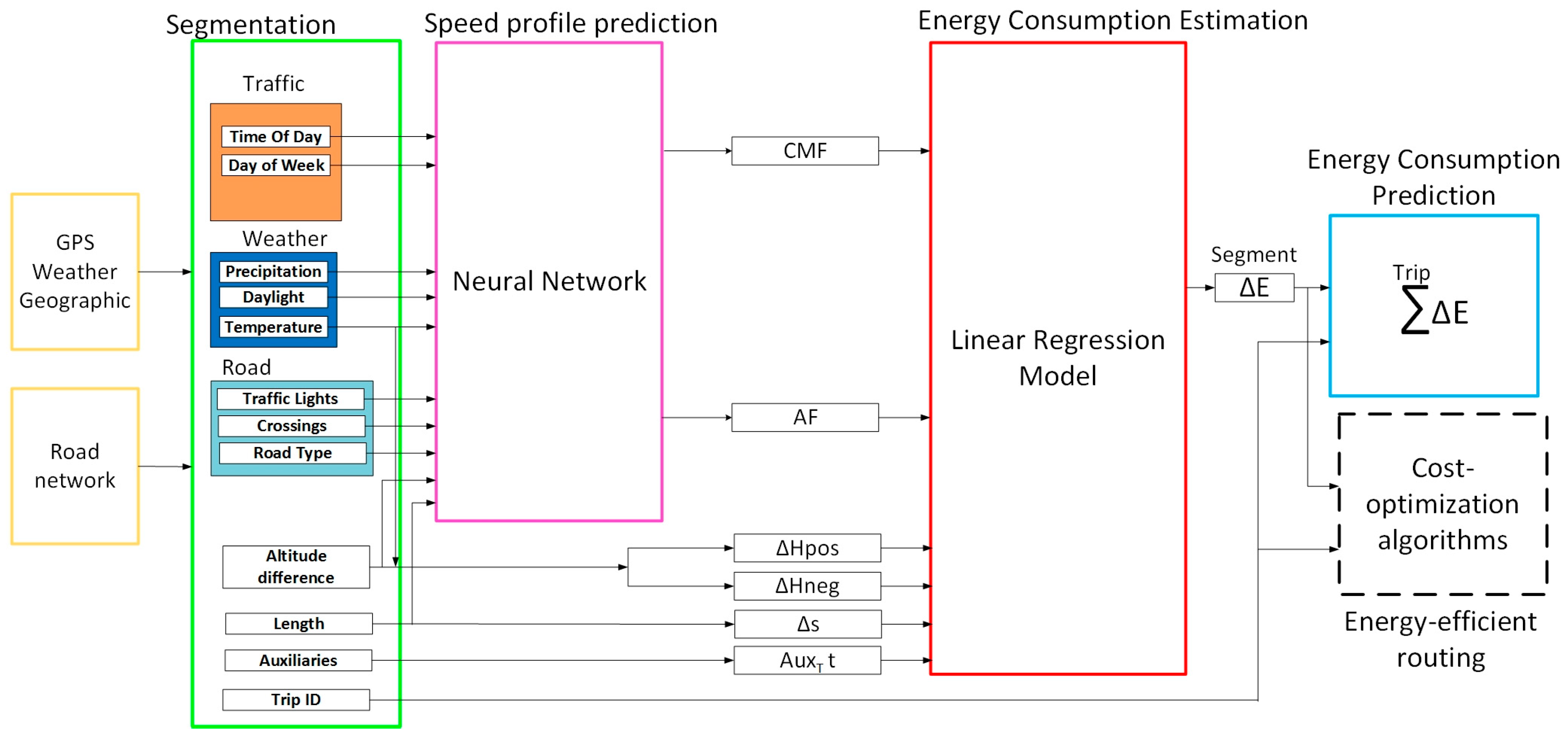
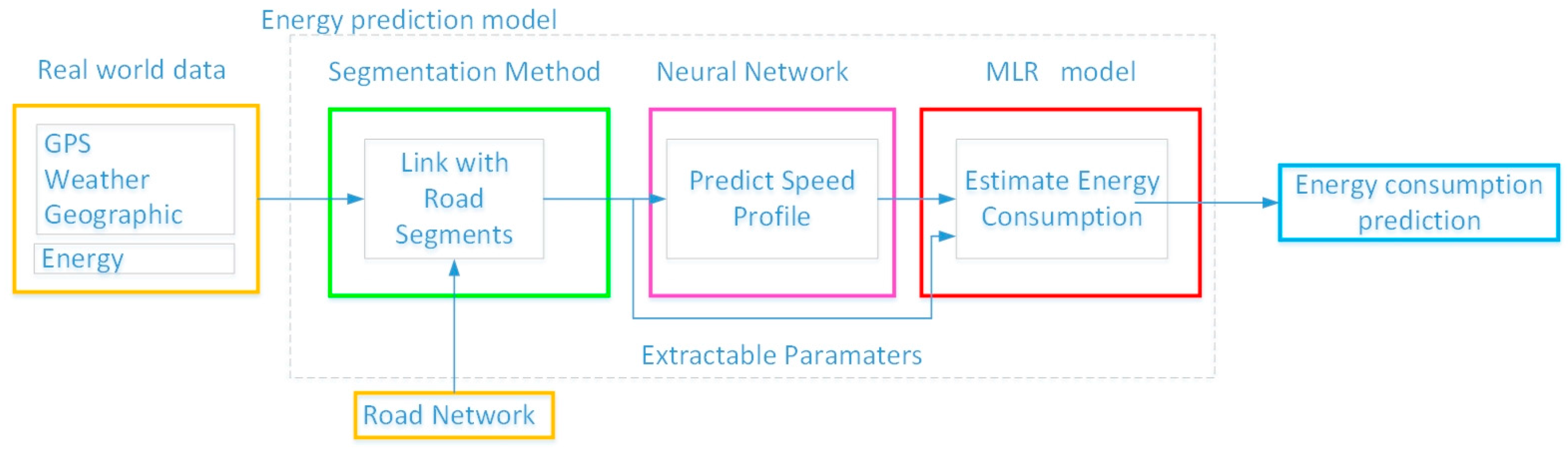
2. The Proposed Energy Prediction Model

The proposed method applies a machine learning technique and a statistical method to real-world measured driving data and energy consumption data of EVs, weather data and geographical information. The real-world driving, energy, weather, and geographical data are first linked to the road characteristics of the individual road segments by location, using global positioning system (GPS) coordinates. The data are then used to train a NN that predicts the speed profile (translated into microscopic driving parameters) from the road characteristics, weather and traffic-related parameters, and construct an energy consumption estimation model using multiple linear regression (MLR). The regression model estimates the energy consumption based on some measurable road and external parameters, and the predicted values for the microscopic driving parameters from the NN. A schematic overview of the proposed energy prediction method, its inputs and output and flow of calculations is given in Figure 1.

Although the flow of calculations moves as indicated in Figure 1, the logic for the layout of the proposed method was derived in another sequence. To provide the reader the same feel and logic behind the build-up of the model, the individual parts of the proposed method will be presented in the same order as they were developed. In the remaining part of this section, first a description of the available data is given, then the energy consumption estimation model is presented, followed by the method to link the vehicle monitoring data with the road network (segmentation method), and finally the NN for speed profile prediction is presented.

2.1. Description of the Available Data

The model is built by combining information from datasets originating from different sources. The data consists of vehicle monitoring data, a road network database, weather data and an altitude map. The vehicle monitoring data consists of two datasets. One dataset consists of 30 EVs which were monitored for a period of more than 1 year. The vehicles were monitored as part of the Flemish Living Labs project EVteclab [31,32]. These vehicles are of the Ford Connect EV model, which is a Ford Connect transformed to an EV drivetrain by the Punch Powertrain company [33]. The vehicles were monitored with a logger that measured both GPS data and data from the vehicle controller area network (CAN). The GPS data were logged at a 1 Hz frequency, the CAN data at a 5 Hz frequency. The GPS data provided the timestamp, latitude, longitude, and vehicle speed. Vehicle accelerations are calculated as the discrete derivative of the GPS speed. Although GPS speed measurements themselves are accurate, the 1 Hz measurement frequency can introduce some loss of accuracy, especially in the calculations of the accelerations. The CAN data provided information on the energy consumption in the form of battery voltage, current and SoC. This dataset will be referred to as Dataset 1. The second dataset concerns three 2014 Nissan Leaf used as taxis in the Brussels Capital Region. They are driven 24/7 by multiple drivers per vehicle. As for Dataset 1, the GPS is logged with a 1 Hz frequency, while the CAN-bus data is logged with a 1 Hz frequency. This dataset will be referred to as Dataset 2. The vehicle specifications of both vehicles are presented in

Table 1. Overview of the vehicle specifications of both vehicle models in the two datasets. EV: electric vehicle.

Reference Name	Vehicle Model	Mass (kg)	Motor Power (kW)	Top Speed (km/h)	Torque (Nm)	Battery Capacity (kWh)	Driving Range (km)
Dataset 1	Punch Powertrains Ford Connect EV	1900	60	120 (limited)	300 (limited)	27	130
Dataset 2	Nissan Leaf (2014)	1601	80	144	300 (limited)	24	199

.

The road database consists of data on the Belgian road network, where the monitored vehicles were predominantly driven. The road network database has navigating capabilities and contains information per segment such as road type, segment length, expected speed over the segment and whether the road was a one-way road, a bridge or a tunnel. The database did not contain any information on the presence of traffic lights and pedestrian crossings, nor did it mention the local speed limit. For the Brussels Capital Region, the road database information was extended with the presence of pedestrian crossings, traffic lights and speed bumps by adding these layers, provided by Brussels UrbIS^®©, to the base road network. The vehicles in Dataset 1 were driven in a mix of highway, rural and urban roads, while the vehicles in Dataset 2 were predominantly driven in a dense urban road network.

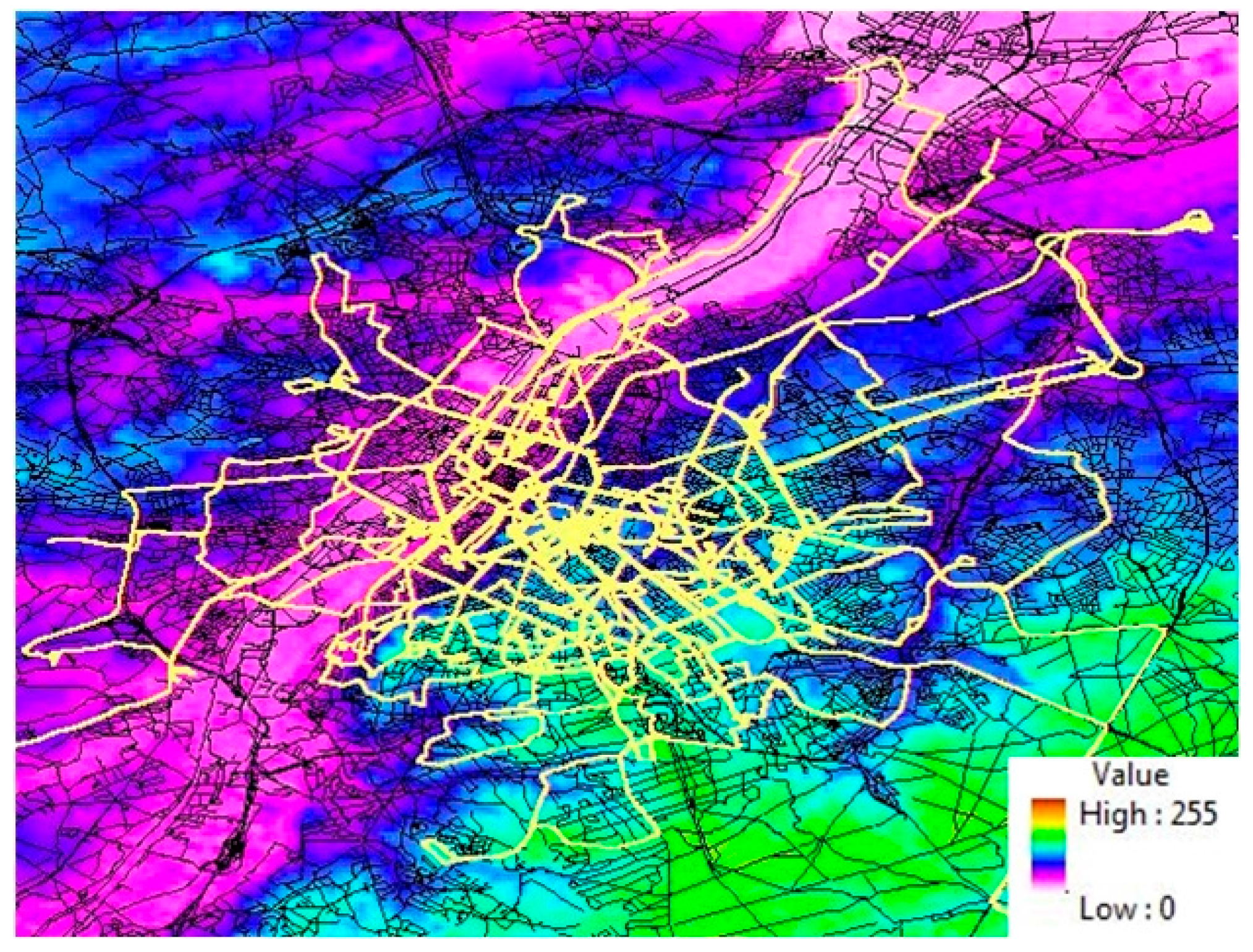
The geographical data consists of a 3 arc-second precision digital elevation map (DEM) coming from the shuttle radar topography mission (SRTM) that provides altitude information on the major part of the globe. The altitude information was extracted from the DEM for each GPS coordinate of the driving data with the use of the geographic information system (GIS) software ArcGIS. To link the driving data to the road network, their GPS coordinates and the road database were joined spatially. The resulting dataset is thus a combination of vehicle GPS data, road information per segment and altitude. To visually illustrate the data, Figure 2 shows the road network in the Brussels Capital Region with part of Dataset 2’s driven trips and the color-scaled altitude map as used in ArcGIS.

The weather data was measured and provided by the Royal Meteorological Institute (RMI) of Belgium and contained temperature, wind speed and direction, and precipitation on an hourly basis for weather stations close to the respective regions in Flanders (Flanders, Belgium) where the vehicles of each dataset were driven. The weather data are considered sufficiently accurate and representative for the whole of the vehicle monitoring datasets because of the limited area of the regions where the vehicles were driven.

As the procedure to link the altitude and road information with the GPS coordinates is computationally intensive, only a representative selection of the vast amount of vehicle monitoring data was taken to establish the scientific value of the proposed methodology. The selection is considered representative if it covers a sufficient part of the road network (i.e., all types of roads) under various conditions. Therefore, the selection for Dataset 1 contained multiple vehicles driven in different parts of the region, on a variety of road types and spread out over multiple months of monitoring. After filtering the selected data, the used data consisted of 3700 km driven by three different vehicles for Dataset 1 and 10,700 km driven by 2 vehicles in Dataset 2.

2.2. Energy Estimation Model

The model is based on the underlying physical model that describes the forces acting on a vehicle in motion. The mechanical energy dE required at the wheels to cover the distance ds is written as:

$$dE=\frac{1}{3600}\left[mg\left(fcos\phi +sin\phi \right)+\frac{1}{2}(\rho C_{x}A\frac{{(v_{EV}+v_w)}^2}{3.6})+\left(m+m_f\right)\frac{dv}{dt}\right]ds$$

(1)

$dE$	Mechanical energy required at the wheels to drive a distance $ds$ [kWh]
$m$	Total vehicle mass [kg]
$m_f$	Fictive mass of rolling inertia [kg]
$g$	Gravitational acceleration [m/s2]
$f$	Vehicle coefficient of rolling resistance [-]
$\phi$	Road gradient angle [°]
$\rho$	Air density [kg/m3]
$C_x$	Drag coefficient of the vehicle [-]
$A$	Vehicle equivalent cross section [m2]
$v_{EV}$	Vehicle speed between the point $i$ and the point $j$ [km/h]
$v_w$	Wind speed projected to the opposing direction of the driving direction [km/h]
$ds$	Distance driven from point $i$ to point $j$ [km]

The terms in (1) represent respectively the rolling resistance, potential energy, aerodynamic loss and inertial energy. Assuming in a first order the rolling resistance coefficient, drag coefficient, air density and vehicle mass are constant, the energy consumption can be described as a linear combination of the kinematic parameters ds, v² ds, $\frac{dv}{dt}$ ds, and h = ds sin$\phi$. To represent the consumption of the auxiliaries, the formula was then extended with a time-linear, temperature scaled term. The simplified linear representation of the energy consumption of the EV can now be written as:

$$E_{EV}=B_1 s+B_2 {(v_{EV}+v_w)}^2 s+B_3 a s+B_4 h+B_{5}Au{x}_{T}Au{x}_{t}t$$

(2)

$Au{x}_T$	Temperature scaling
$Au{x}_t$	Fraction of time the auxiliaries are switched on
$t$	Time
$s$	Distance

By applying MLR to the real-world driving and energy data, the coefficients of the linear combination in (2) are determined. The effect of wind speed on energy consumption does not feel as very significant because, in general, wind speed is moderate compared to vehicle speed and driving direction during driving mostly shifts frequently. However, upon close examination of the outliers in results of the energy estimation using (2), it was established that the wind can have a large influence on energy consumption in some cases. Therefore, wind speed was added to the predictor variables in (2) by projecting it on the driving direction. 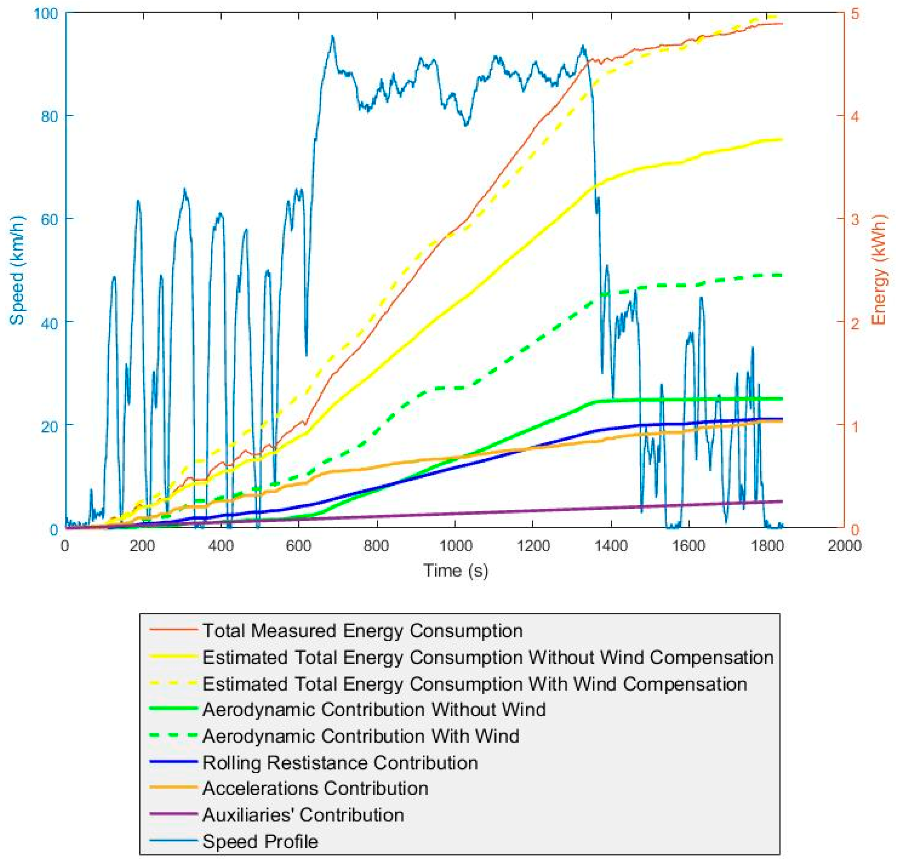Figure 3 presents an example of energy consumption estimation using (2) for a measured trip with reported heavy headwinds. It depicts the individual contributions of the regression terms in a cumulative way along the progression of a trip, with and without the superposition of headwind on the speed predictor. Superposing the projected wind speed to the vehicle speed in the aerodynamic term of the energy equation reduced the error from around 30% to only a few percent over the trip.

The sensitivity analysis of the energy demand, presented in [34], highlights the effect of a variable rolling resistance and, to a lesser extent, vehicle mass on the energy consumption of the EV. The rolling resistance coefficient can vary considerably because of many factors, such as road surface, road wetness, tires and tire pressure, with reported variations up to 65% [22,35], and therefore require extensive measurements to characterize it. There also exist methods to estimate vehicle mass and the rolling resistance coefficient online [36]. If explicit measurements of rolling resistance and vehicle mass are available, these parameters can easily be drawn out of the regression coefficients and added explicitly to the predictors in (2) to account for their variability.

By constructing the model using the MLR based on the vehicle dynamics equation, the method is both computationally simple and increases interpretability through the causal relations in the model. To allow the MLR to detect the individual influences on the energy consumption more easily, the trips are split into shorter segments, so more variability resides in the measured data.

2.3. Segmentation Method

The trips can be split into shorter segment with more distinct conditions to avoid over-aggregation and a loss of variability in the data. The energy estimation is done on these segments and are later recombined for an estimation on trip level. Based on (2), the formula for the simplified linear representation of the energy consumption in function of its predictors now becomes:

$$\begin{array}{cc}\Delta E\hfill & ={\displaystyle \sum }\Delta Esegments\hfill \\ & ={\displaystyle {\displaystyle \sum }_{segments j}^{trip}}[B_1 \Delta s_j+B_2{\displaystyle {\displaystyle \sum }_i^n}{({v_{EV}}_i+{v_w}_i)}^2\Delta s_i+B_3 \left(CM{F}_j^{+}\right) \Delta s_j\hfill \\ & +B_4 \left(CM{F}_j^{-}\right) \Delta s_j+B_5\Delta Hpo{s}_j*+B_6 \Delta Hne{g}_j+B_7 Au{x}_{T_j}\Delta t_j+\epsilon ]\hfill \end{array}$$

(3)

with:

$$CM{F}_j=\frac{{{\displaystyle \sum }}_{i=2}^n\left|v_{EV}{{}^2}_i-v_{EV}{{}^2}_{i-1}\right|}{\Delta s}$$

(4)

$$A{F}_j={\displaystyle \sum }_i^n{({v_{EV}}_i+{v_w}_i)}^2\Delta s_i$$

(5)

while:

• $B_i: \mathrm{regression}\mathrm{coefficients}$
• $\Delta E: \mathrm{energy}$
• ${v_{EV}}_i: \mathrm{vehicle}\mathrm{speed}\mathrm{at}\mathrm{time}{t}_i$
• ${v_w}_i: \mathrm{wind}\mathrm{speed}\mathrm{value}\mathrm{projected}\mathrm{on}\mathrm{the}\mathrm{driving}\mathrm{direction}\mathrm{at}\mathrm{time}{t}_i$
• $\Delta s: \mathrm{distance}$
• $\Delta s_i: \mathrm{distance}\mathrm{driven}\mathrm{between} t_{i-1}\mathrm{and} t_i$
• $Au{x}_T: \mathrm{temperature}\mathrm{scaling}$
• $Au{x}_t: \mathrm{fraction}\mathrm{of}\mathrm{time}\mathrm{auxiliaries}\mathrm{are}\mathrm{switched}\mathrm{on}$
• $\Delta t: \mathrm{time}$
• $\Delta Hpos: \mathrm{positive}\mathrm{elevation}\mathrm{changes}$
• $\Delta Hneg: \mathrm{negative}\mathrm{elevation}\mathrm{changes}$
• $\epsilon : \mathrm{error}\mathrm{term}$
• $n: \mathrm{number}\mathrm{of}\mathrm{data}\mathrm{points}\mathrm{in}\mathrm{segment}j$

The constant motion factor (CMF), defined in (4), is the sum of kinetic energy changes per unit distance and is equivalent to the acceleration term in (2). Because the sum of the positive and negative kinetic energy changes over a segment are not necessarily equal, they are split up in CMF⁺ and CMF⁻ in (3). The CMF and aerodynamic factor (AF), defined in (5), are a translation of the speed profile for this method and represent respectively the performed accelerations and driving speed.

The method to split the trips into micro-trips or segments is an important part in the complete proposed method. The simplified linear representation of the energy consumption expressed in (3) requires a minimum of aggregation of data points, but over-aggregation of the predictors leads to loss of variability. A common practice in many analysis [37] consists of splitting trips into micro-trips of equal duration. However, this method leads to an arbitrary division in segments, as there is no link between the road characteristics and the segments. By splitting the trips into segments in an arbitrary way, driving and road conditions are not represented uniformly over the segments and their representation cannot be controlled. Additionally, splitting trips into segments of equal duration makes the duration predictor constant, making it hard to detect its relation to the dependent variable through linear regression. One method to divide trips into segments with variable duration is to link the data points to the road segments by location. The segment length will then be variable and the speed profile allocated to a specific road segments with its own characteristics. This method is therefore the most sensible with respect to the complete proposed method. Applying this segmentation method, the length of the obtained segments depends entirely on the length of the road segments. The road segments’ lengths range from a few tens of meters up to three kilometers, with a high concentration of very short segments. For very short segments, the number of data points per segment become too low to obtain accurate results. Hence, sequential very short segments within one trip (containing less than 100 data points) with identical road types were aggregated to combined segments up to 100 data points.

2.4. Speed Profile Prediction

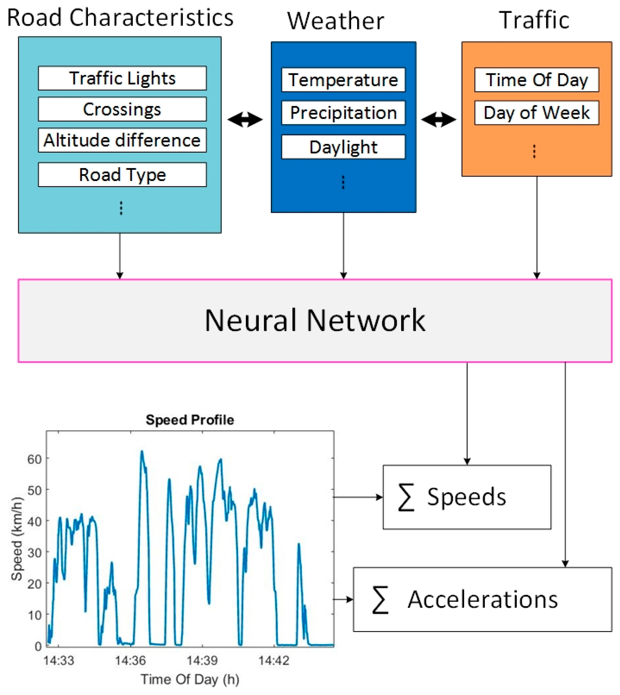
In the energy model presented above, the speed profile is translated into two predictors: the speed-related AF and the acceleration-related CMF. The AF and CMF are highly variable and unknown prior to departure. All other predictors in (3) are either known or directly measurable for a chosen route. To be able to predict the energy consumption over the route, the values of these two predictors of the energy estimation model must be predicted. If we want to enable energy-efficient routing, this prediction must be done for each individual segment of the road network to allocate an energy cost. Because the interactions between the road characteristics, traffic situation and driver are complex and likely to have non-linear and interdependent relations with the driving speed and accelerations performed, the decision was taken to develop a model based on machine learning. The estimation technique used is a neural network (NN) [38]. The NN is a powerful technique for black box function approximation, capable of predicting non-linear, complex relations. A NN is trained to link attributes from the road and the traffic of the road segments with the actual measured AF and CMF. Figure 4 illustrates the principle of the NN inputs and outputs.

The available road-related attributes were the road type, altitude differences, indication of the average speed, and crossings, and were extended with presence of traffic lights, speed bumps and pedestrian crossings for Dataset 2. In case sequential very short segments of the same road type were aggregated to have sufficient data points, as explained in Section 2.3, their road related attributes were aggregated as well. The traffic light information was added as static information to the road database and merely indicates its presence on a segment, without information on signal phases. The crossings were categorized as left turn, right turn, straight through and were categorized according the magnitude of the angle. The measured average speed over a segment could have been used as a predictor, as the real-time average speed can be imported using real-time traffic services. However, because no data from traffic services were available that would allow verification of this assumption, it was opted not to do so and have a more conservative performance of the prediction. The dataset did not contain explicit characteristics of traffic, but the weather characteristics (temperature and precipitation), time of the day, and day of the week were considered implicit indicators of traffic state. Although the prediction of CMF and AF by the NN is based on many road-related attributes, weather characteristics and implicit traffic indicators, these parameters do not comprise of all the attributes, or account for all complex interactions that influence the speed profile. Unique events, such as accidents, sport events or road works, will have an influence on the traffic state [39,40]. Individual driving style can modify the speed profile, while the traffic light status can change it fundamentally. As this information was not present in the available datasets, it presents some limitations of the model in its current state.

3. Results

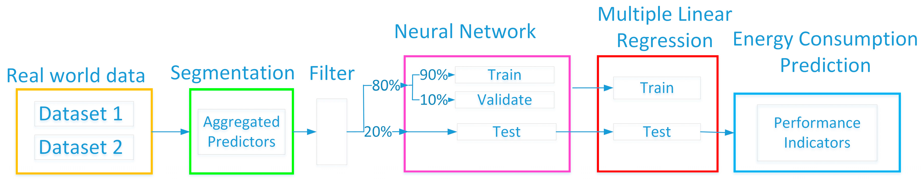
The proposed model is a combination of a NN for the prediction of the CMF and AF (representing the speed profile) on the road segments, followed by the MLR model to estimate the energy consumption from the predicted CMF, the predicted AF, and the remaining measurable parameters in (3). Based on the schematic overview of the model, presented in Figure 1, a detailed overview of the proposed model with its inputs and outputs is given in Figure 5.

To construct the data-driven model, the selected datasets are first split up into 80–20% for training-testing of the entire model as a cascade of the NN and MLR. The 80% for training is then split up in 90% in training and 10% in validation of the NN specifically. The data partitioning and data process flow is illustrated in Figure 6.

There is no specific test set for the NN, as the test set will serve to evaluate the complete cascade model. The filtering process focused on mainly three issues: the correct spatial joining between the GPS coordinates and the road database (for example if the vehicles drove on a factory site—the spatial joining would then incorrectly link those GPS points to the nearest road segment), the correct synchronization between the CAN data and GPS data, and the occurrence of a charging event during the segment. The results of the energy estimation model, NN prediction and the complete proposed model for energy consumption prediction will be presented in Section 3.1, Section 3.2 and Section 3.3 respectively.

3.1. Energy Estimation Model

Applying the MLR with the segmentation based on (3) for Dataset 1 and Dataset 2 result in the correlation coefficient, regression coefficients and p-values presented in

Table 2. Overview of the regression coefficients and p-values for energy estimation model based for Dataset 1 and Dataset 2.

MLR Results of the Energy Estimation Model
Coefficient		Intercept	Rolling Resistance (B1)	Aerodynamic (B2)	Positive Accelerations (B3)	Negative Accelerations (B4)	Positive Altitude (B5)	Negative Altitude (B6)	Auxiliaries (B7)
Dataset 1 R2 = 0.96	Bi	−0.0071	0.0670	1.10 × 10−5	2.75 × 10−5	1.64 × 10−5	0.00423	0.00389	0.136
	p-values	<0.5	<0.0001	<0.0001	<0.0001	<0.0001	<0.0001	<0.0001	<0.0001
Dataset 2 R2 = 0.93	Bi	−0.0024	0.0541	5.23 × 10−6	1.92 × 10−5	1.21 × 10−5	0.00341	0.00259	0.297
	p-values	<0.05	<0.0001	<0.0001	<0.0001	<0.0001	<0.0001	<0.0001	<0.0001

. Comparison of the results for Dataset 1 and Dataset 2 shows that the energy estimation model is vehicle-specific—as the regression coefficients are different—but have similar order of magnitudes and trends. All p-values for the regression coefficients B₁–B₇ are below 0.0001, indicating these terms are very significant. The MLR also generates an intercept, which is a constant term (or offset) that equals the prediction when all predictors are zero. However, the vehicle dynamics in (1), leading to the simplified linear representation of the energy consumption in (2), do not have a constant term. This means no physical interpretation can be given to this intercept term and a part of the variability which is not explained by the model is contained within the intercept term for a better fit.

For both datasets, the coefficient for the positive altitude changes is larger than the coefficients for the negative altitude changes, which is physically correct as only part of the potential energy will be recovered in kinetic energy or electrical energy through regenerative braking. The ratio of the negative to the positive coefficient for Dataset 2, 0.00259/0.00341 = 76%, is consistent with the typical drivetrain efficiency [5] and efficiency of regenerative braking [41]. However, for Dataset 1 this value of 0.389/0.423 = 93% is high. It should also be mentioned that for Dataset 1, the value of these coefficients was sensitive to the trips contained in the dataset and had subsets where the negative coefficient was larger than the positive, which is physically impossible because it would mean more energy is recovered during downhill than what was consumed during uphill. In energy-efficient routing this must be avoided because it will potentially lead to a suggestion of routes with many altitude differences instead of avoiding them. The reason for the sensitivity of the coefficients for the altitude contribution in Dataset 1 is suspected to be the small variability of the altitude in the geographic region of Dataset 1, which makes it harder to detect its influence in the variability of the energy consumption. However, because the altitude differences are so small in this region, this will also introduce low average absolute errors compared to the total energy estimation.

3.2. Speed Profile Prediction

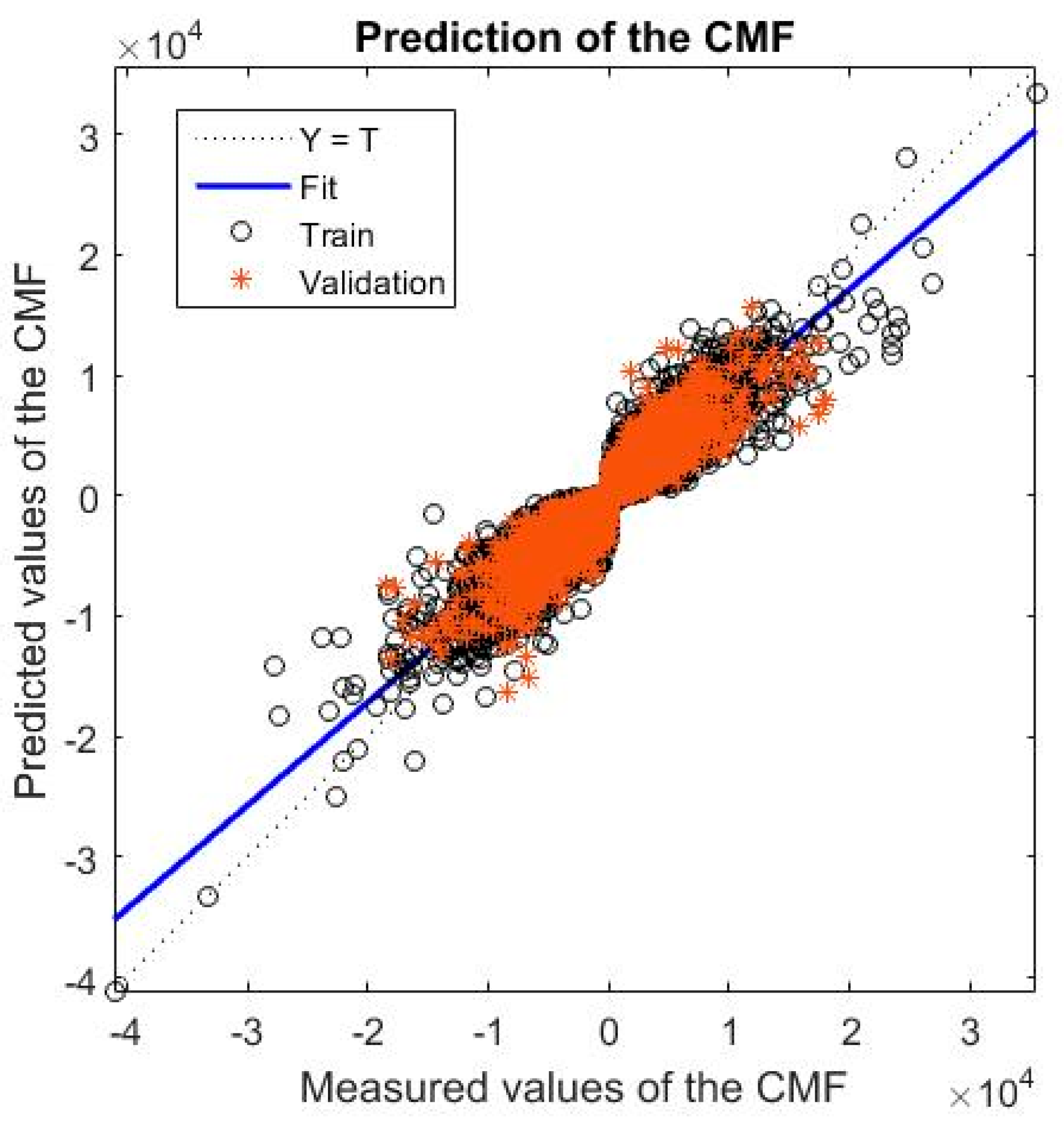
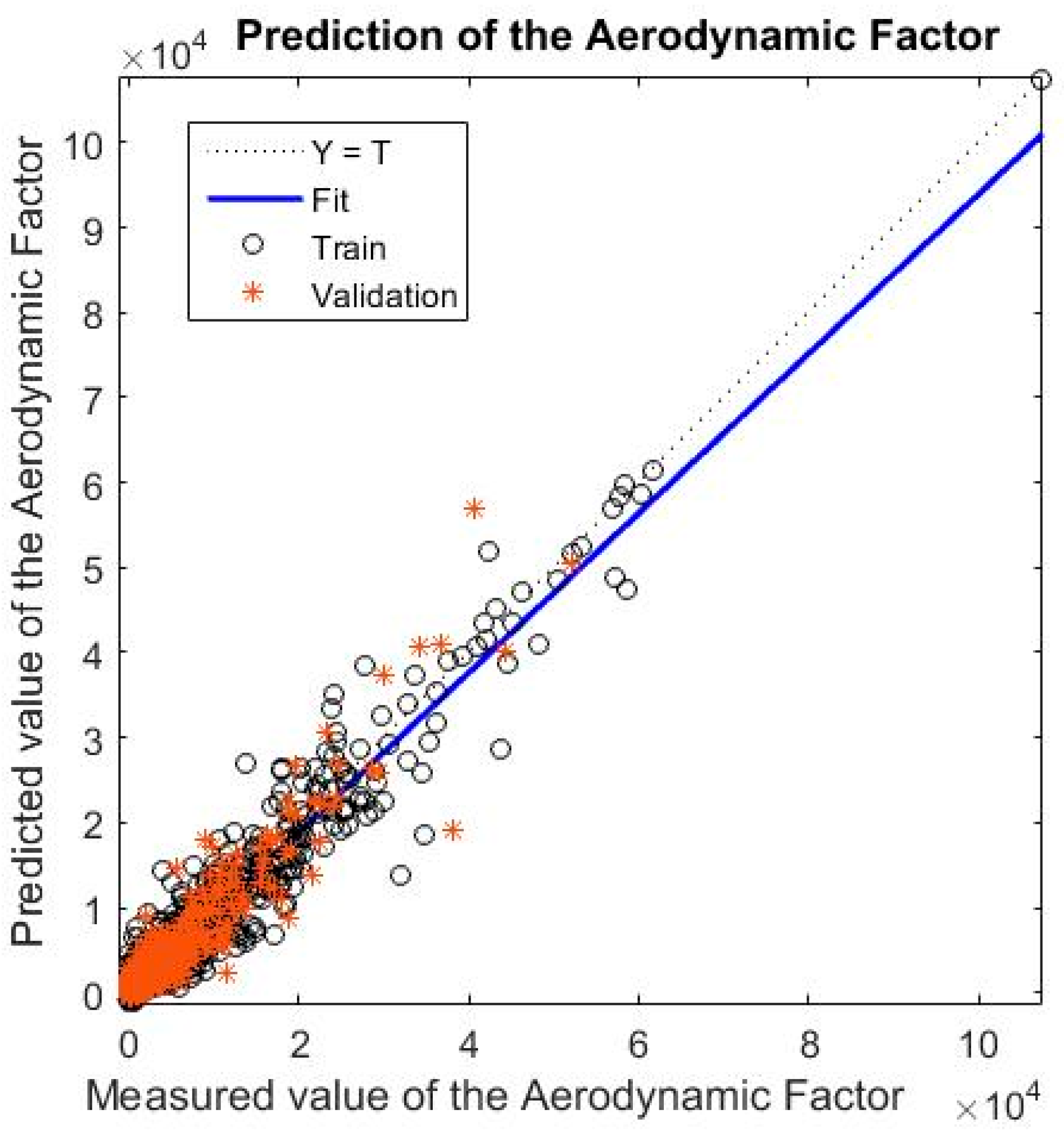
The data for the NN is split up into 90% for training and 10% for validation. The regression plots for the prediction of the AF and CMF on Dataset 2 are given in Figure 7 and Figure 8.

The correlation coefficient of 0.97 and 0.93 for the two respective predictions is high. However, there is a spread of the data points around the blue line, especially for the CMF prediction, which indicates not all the variability is explained by the current predictors. This is due to the fact that the driven speed and accelerations are complex variables with a lot of interdependent influencing factors and they are sensitive to random events. When including explicit information on traffic density and driving style, more variability of the data can be explained, similarly to what was observed after including the traffic lights and speed bumps in Dataset 2.

Table 3. Correlation coefficient (R) and mean squared error (MSE) for the prediction of the AF and CMF for both Dataset 1 and Dataset 2.

Variable	Dataset 1		Dataset 2
	R	MSE	R	MSE
AF	0.97	2.57 × 106	0.97	4.17 × 105
CMF	0.91	5.37 × 106	0.93	9.37 × 105

presents the correlation coefficient R and the mean squared error (MSE) for the prediction of the AF and CMF for both Dataset 1 and Dataset 2. The values obtained in Table 3 have a very stable behavior when calculated multiple times.

According to the values presented in Table 3, the NN is more performant for Dataset 2. This is attributed to the extension of the input parameters for the prediction with traffic lights, pedestrian crossings and speed bumps in Dataset 2. This information was not available in Dataset 1. However, the large difference in the MSE between the 2 datasets is also partly due to the different sizes of the road segments in both sets. On average, the larger road segments in Dataset 1 will cause larger absolute errors with similar relative errors.

3.3. Energy Consumption Prediction Model

The proposed method is a combination of the MLR for the energy consumption estimation, based on the vehicle dynamics equation, and a NN for the prediction of the speed profile. Using a multistep model can lead to an increased loss of accuracy as the error is accumulated in each step. To benchmark the results, the results of the proposed model were compared to two other models. The first benchmark model is a NN prediction that was trained with the same parameters as the proposed model in the input, and the energy consumption in the output. The second benchmark model is a simple calculation of the energy consumption by multiplication of the distance with the total real-world measured average energy consumption. The models’ performance will be analyzed through two absolute error indicators which are calculated on the part of the data preserved for testing: root-mean-square error (RMSE) and mean absolute error (MAE). If the error is defined as the target value $(v_t)$ minus the predicted value $(v_p)$, the indicators are calculated as:

$$\epsilon = \left(v_t-v_p\right)$$

(6)

$$RMSE=\sqrt{\frac{{{\displaystyle \sum }}_1^n{\epsilon }^2}{n}}$$

(7)

$$MAE= \frac{{{\displaystyle \sum }}_1^n\left|\epsilon \right|}{n}$$

(8)

The root-mean-square error penalizes the predictions far off target. The performance indicators for the NN–MLR model and the two benchmark models for Dataset 1 and Dataset 2 are presented in

Table 4. Performance indicators for the energy prediction model and the two benchmark models for comparison on segment level. RMSE: root-mean-square error; MAE: mean absolute error; <E>: average consumed energy per segment.

Dataset	Performance Indicator	NN–MLR Prediction	NN Prediction	Average Consumption Prediction	<E> (kWh)
Dataset 1	RMSE (kWh)	0.0733	0.0923	0.0723	0.159
	MAE (kWh)	0.0516	0.0615	0.0503
	MAE/<E>	0.32	0.38	0.32
Dataset 2	RMSE (kWh)	0.0267	0.0335	0.0341	0.0336
	MAE (kWh)	0.0190	0.0230	0.0232
	MAE/<E>	0.57	0.68	0.69

also indicates the average consumed energy per segment, <E>, for both datasets.

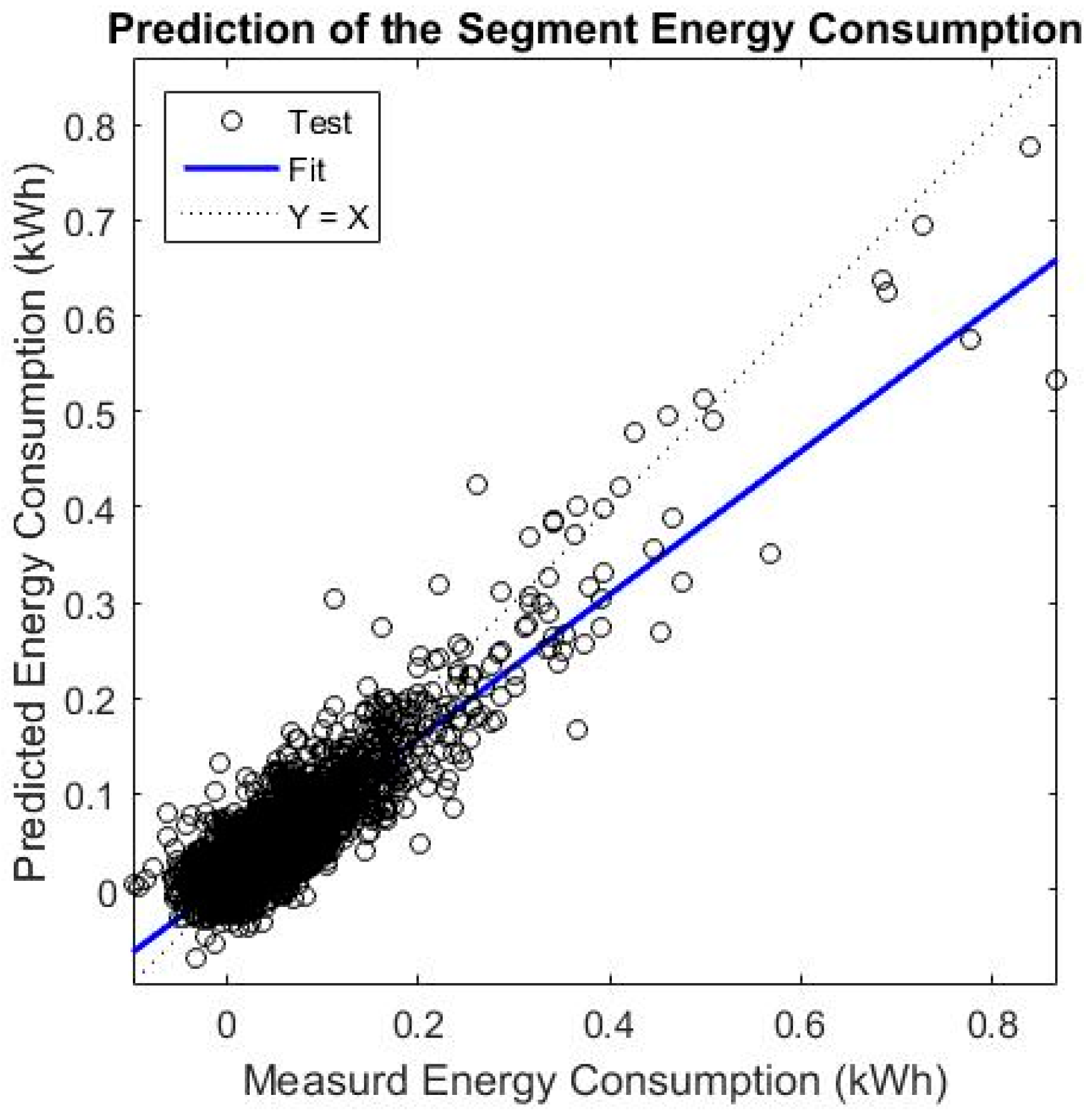
Regarding the performance indicators, Table 4 shows that for Dataset 1, the NN–MLR and average consumption predictions have a similar performance and outperform the direct NN prediction. For Dataset 2, the NN–MLR clearly outperforms the two other prediction methods, which have a similar performance. This is consistent with the observation from Table 3 in Section 3.2, which showed that the prediction of the AF and CMF had better results in Dataset 2 due to the presence of traffic lights and speed bumps in the NN predictors. The performance of all three prediction methods is significantly lower in Dataset 2 compared to Dataset 1. This can be explained by the difference in the composition of the road network of both datasets. Dataset 1 contains a mixture of highway, rural and urban roads, with a considerable number of rural roads, while Dataset 2 primarily consists of dense urban roads. This results in significantly shorter road segments with much more diverse conditions and lower average energy consumption. This also contributes to the power of the NN prediction stage in the NN–MLR and its better performance for in Dataset 2. To visualize the energy consumption prediction for the individual segments, the regression plot for the prediction of the energy consumption of the segments in Dataset 2 in given in Figure 9.

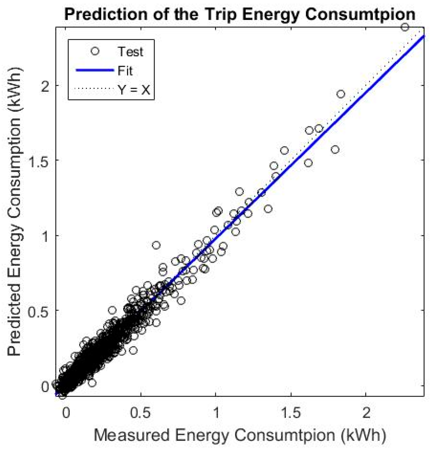
If the segments are recombined to the original trips, we can evaluate the performance of the prediction methods on trip level. The same performance indicators for the prediction of the segments are calculated for the trips and presented in

Table 5. Performance indicators for the energy prediction model and the two benchmark models for comparison on trip level.

Dataset	Performance Indicator	NN–MLR Prediction	NN Prediction	Average Consumption Prediction	<E> (kWh)
Dataset 1	RMSE (kWh)	0.605	0.539	0.471	2.4
	MAE (kWh)	0.335	0.364	0.316
	MAE/<E>	0.14	0.15	0.13
Dataset 2	RMSE (kWh)	0.142	0.178	0.178	0.78
	MAE (kWh)	0.0917	0.119	0.119
	MAE/<E>	0.12	0.15	0.15

. The performance indicators on trip level have the same trend as on segment level: the average consumption prediction performs best for Dataset 1 by a small margin, the NN–MLR performs best in Dataset 2 by a significant margin. The values of the MAE per average consumed energy decreases significantly for the prediction on trip level. This is because the errors on the segment prediction are symmetrically distributed and partly cancel each other out when recombined to trips. To visualize the energy consumption prediction for the individual trips, the regression plot for the prediction of the energy consumption of the trips in Dataset 2 is given in Figure 10. The figure demonstrates the good results for the NN–MLR prediction on trip level.

To evaluate how much of the prediction error in the NN–MLR is attributed to the MLR, the measured values of the CMF and AF can be inserted into the MLR, instead of the predicted values by the NN stage.

Table 6. Performance indicators MLR energy estimation model on trip and segment level by considering the measured CMF and aerodynamic predictor as input.

Indicator	Dataset 1			Dataset 2
	RMSE	MAE	MAE/<E>	RMSE	MAE	MAE/<E>
MLR estimation for segment	0.0350	0.0231	0.15	0.0146	0.0133	0.39
MLR estimation for trip	0.275	0.170	0.071	0.465	0.0663	0.085

shows the performance indicators on segment and trip level of for Dataset 1 and Dataset 2, in the case the measured values of the AF and CMF are the inputs to the MLR. The results show a MAE of 7.1% and 8.5% of the mean energy consumed per trip for Dataset 1 and Dataset 2, respectively. This represents approximately half of the mean error created by the NN–MLR. It is important to observe the high value of MAE/<E> for the estimation on the segments in Dataset 2. The large error for short segments demonstrates the incapability of the MLR to estimate the instant power consumption and the need for aggregation of data points.

The results presented here are averages for the prediction on segments originating from a random selection from all road segments in the datasets, which are not limited to a specific selection of an area in the road network or specific road types (such as highway or arterials), as is often done in literature [29]. The NN–MLR has a better overall performance than the two benchmark models and has several other advantages. It performs significantly better when diverse conditions that influence energy consumption and driving behavior are present. This illustrates the power of a NN in the prediction of these non-linear systems. If the energy consumption is close to the average energy consumption (in less diverse conditions), the NN–MLR loses part of its advantage compared to the average consumption model, because, by cascading both models, the error produced in the NN is propagated in the MLR. However, cascading both models grants more flexibility and preserves the link with the underlying physical relationships. This facilitates interpretation of (causal) relations between the inputs and outputs of the model.

4. Conclusions

This paper presents a data-driven energy consumption prediction method for EVs, suited for energy-efficient routing. It uses a cascade of a NN and a linear regression model. The MLR model is used to estimate the energy consumption, given a number of predictor variables, while the NN serves to predict the unknown predictor variables (inputs) of the MLR. The proposed method predicts the energy consumption on the individual segments of the road network, allowing a cost allocation to each link in the road network, so cost-optimization algorithms can define energy-efficient routes. The MLR is performed on smaller parts of trips (segments) to capture more variability in the data. It was decided to segment the trips based on the actual road segments in the network instead of an arbitrary division in order to allocate driving parameters to the road characteristics of the segments. The NN is trained to predict the speed profile, here translated in an AF and CMF (representing accelerations), from road-, traffic-, and weather-related attributes. It is the cascade of first the NN for speed profile prediction and thereafter the regression for energy estimation that form the proposed energy prediction model. To evaluate its performance, the proposed NN–MLR model is compared to two benchmark models. A first benchmark model is a NN that directly predicts the energy consumption from the road and traffic related attributes, omitting the regression part, and the second benchmark model is a simple estimation calculated with the total average consumption. The NN–MLR prediction has an overall better performance than both benchmark models. In a dense urban environment, subject to more diverse conditions, the NN–MLR prediction has a significantly better performance than the other two. When recombined to trips, the performance increases as errors on segments are symmetrically distributed and partly cancel each other out. For the proposed complete energy prediction model, approximately half of the total error can be allocated to the NN prediction of the CMF and AF. The proposed NN–MLR has a MAE that is 12–14% of the average trip consumption of which only 7–9% is caused by the MLR energy estimation itself. These results are averages for the prediction originating from a random selection from all road segments in the datasets, and is not limited to a specific selection of an area in the road network or specific road types, as is often done in literature.

The model results show it is, on average, able to predict the energy consumption more precisely than an average consumption model. It distinguishes different energy consumption influencing factors per road segment (such as road characteristics, weather, altitude differences), making this approach suited for energy consumption prediction for any given road in the network prior to departure and enables cost-optimization algorithms to calculate energy-efficient routes. Furthermore, by separating the model in a stage for the prediction of the speed profile and a stage for the energy consumption estimation (MLR), it benefits from the power and flexibility of data mining techniques, while preserving the interpretability of the results because of the preserved link with the underlying physical model. The data-driven approach allows this method to be easily applied to other EVs and allows for the developed model to be easily updated over time to adjust to changing conditions.