A Top-Down Spatially Resolved Electrical Load Model

Abstract

The increasing deployment of variable renewable energy sources (VRES) is changing the source regime in the electrical energy sector. However, VRES feed-in from wind turbines and photovoltaic systems is dependent on the weather and only partially predictable. As a result, existing energy sector models must be re-evaluated and adjusted as necessary. In long-term forecast models, the expansion of VRES must be taken into account so that future local overloads can be identified and measures taken. This paper focuses on one input factor for electrical energy models: the electrical load. We compare two different types to describe this, namely vertical grid load and total load. For the total load, an approach for a spatially-resolved electrical load model is developed and applied at the municipal level in Germany. This model provides detailed information about the load at a quarterly-hour resolution across 11,268 German municipalities. In municipalities with concentrations of energy-intensive industry, high loads are expected, which our simulation reproduces with a good degree of accuracy. Our results also show that municipalities with energy-intensive industry have a higher simulated electric load than neighboring municipalities that do not host energy-intensive industries. The underlying data was extracted from publically accessible sources and therefore the methodology introduced is also applicable to other countries.

1. Introduction

Due to the rising share of variable renewable energy sources (VRES), such as wind and photovoltaics, the operation of the electrical grid in Germany has become more complex. The fluctuating nature of VRES output complicates any long-term forecast of the electrical grid load, which is necessary for the future grid development. A model of the electrical grid load ought to be spatially resolved in sufficient detail to identify appropriate locations for electricity storage or where unusable surplus power occurs, which can be used, for example, for the so-called Power-to-Gas approach [1,2,3]. Furthermore, with high spatial resolution, effects that arise only locally can be observed.

However, existing models of electrical grids only make use of a rather coarse resolution. The model for Greece in Koltsaklis et al. [4], for instance, is divided into five geographical zones, so as to enable policy makers to utilize the model for planning and scenario analysis. Also for planning purposes, the model of Germany in Ludig et al. [5] is divided into five regions that correspond to the regions observed by transmission system operators (TSO) in the country. Heitmann et al. [6] introduce a more detailed model for Germany that features 29 nodes in an effort to analyze the influence of uncertain and fluctuating parameters such as wind supply on the existing electricity system. In order to quantify the benefits of optimal transmission grid extensions, Fürsch et al. [7] enumerated 224 nodes for the whole of Europe, while Hauer et al. [8] analyzed the power system of the TSO 50 Hertz in Germany and divided it into eight regions, in accordance with the number of directly subordinated distribution grids. In Leuthold et al. [9], one of the most detailed models of the electrical grid is introduced, which consists of more than 2000 nodes for Europe and 365 nodes for only Germany, with the district being the smallest unit of information in terms of spatial resolution. However, as these districts can still be fairly large, they cannot identify effects that emerge at a more local level.

In a bid to address some of these analytical gaps, this paper introduces a model of the electrical grid in Germany at the municipal level, spanning 11,268 nodes. In Section 4, the differences between municipalities of the same administrative district are shown. In municipalities that host energy-intensive industries, the electrical grid is obviously more loaded than neighboring districts that lack these. The data was drawn from publicly accessible sources, and therefore the methodology followed is also applicable to other countries in Europe, e.g., Italy [10,11,12].

In order to calculate the electrical grid load, electrical energy models usually incorporate three elements: electrical load, electrical generation and transmission. In order to evaluate the impact of future developments in power generation, particularly from VRES, this paper analyzes electrical load. Other models use load diagrams based on the monthly billing of households to forecast electrical load in different regions over the long term or analyze consumption profiles from customer categories in combination with data from transforming stations to achieve spatial resolution [13,14,15]. The means of getting an hourly profile by using a monthly bill is the following: first of all, there will be a used weekly standard load profile, for instance from households, which will be summarized for one month. This value will be adjusted to the energy consumed during a month from the monthly energy bill. It is perhaps not an optimal method, but it is used in some fields.

Alternatively, artificial neural networks with input data such as gross national product, gross domestic product, population or industrial production predict future electrical loads for larger areas [16]. Whereas these studies either focus on primarily local data or on data with a notably coarse resolution, our study combines time-resolved grid load data and consumption data from official statistics to improve the accuracy of the model.

Furthermore, many studies are not fully transparent in their assumptions [17,18] (p. 98), while this study introduces a straightforward spatial and time-resolved model of the electrical grid load in Germany that can be used as a basis for more detailed analyses on electrical grid development [19,20], electricity storage [21,22,23] or coupling with other energy systems, such as the Power-to-Gas concept [1,2,24,25].

Section 2 explains possible input parameters for the electrical load and the advantages and disadvantages of each of them. The focus is on values for Germany, but the main conclusions can be transferred to other countries. Section 3 explains in detail the input values that were used to model the spatially-resolved electrical load in Germany. It describes the data needed to increase the spatial resolution from the country level to the regional level. In Section 4, the main results of the simulation are shown.

2. Input Data for the Electrical Load Model

Besides the use of standardized electrical load profiles, an electrical load model can be designed on the basis of measured data. In Germany, there are two sources of information for measured electrical loads: the European Network of Transmission System Operators for Electricity (ENTSO-E) and the four transmission system operators (TSOs) in Germany, namely: Amprion GmbH (Amprion), TenneT TSO GmbH (TenneT), TransnetBW GmbH (TransnetBW) and 50 Hertz Transmission GmbH (50 Hertz). Figure 1 shows a detailed district allocation of Germany’s four TSOs. It is notable that some TSO districts are outside of the core regions of the TSO, e.g., the district of Hamburg, managed by 50 Hertz, is colored orange.

ENTSO-E is an association of 41 TSOs from 34 European countries, including four from Germany [26]. ENTSO-E gathers data from the TSOs, not all of which publish their measurements. The combination of both sources generates precise information on the electrical load.

Furthermore, different types exist to describe the electrical load, hence, the exact definition of electrical load in the respective data must be checked. For our model, possible input parameters regarding electrical load are the vertical grid load and total load. Both will be described in the following sections.

2.1. Vertical Grid Load

According to Hennings et al. [27], the vertical grid load is defined as the “total power transferred from the transmission grid to distribution grids and consumers”. In contradistinction to the other loads, the vertical grid load is the only one that is directly measured [28] (p. 69). The vertical grid load can therefore be calculated with:

$${\mathrm{P}}_{Verticalgridload}={\mathrm{P}}_{\mathrm{Transmission}\mathrm{grid},\mathrm{ij}}-{\mathrm{P}}_{\mathrm{Distribution}\mathrm{grid},\mathrm{ij}}$$

where the hours in the year are $\mathrm{i}=1,2,3,4,\dots 8760$ and quarter-hours for the specific hour are $\mathrm{j}=1,2,3,4$. If the power flow from the Distribution grid is higher than the one from the Transmission grid, the vertical grid load becomes negative. The vertical grid load is the most common input data for electrical load models. However, this approach is flawed, as will be described in the next section, which will also outline what should be changed in future models as the amount of VRES continues to rise.

The specificities of the vertical grid load pertain to the distribution grid as a consumer. This is a viable method as long as power flows only from the transmission grid into the distribution grid. This was the case in the past, when the predominant share of power was provided by centralized fossil fueled power plants that fed into the transmission grid, but since most VRES also feed into the distribution grid, the vertical grid load does not correctly display the load. Figure 2 illustrates the fundamental error associated with using the vertical grid load variable. It shows the power flow for two cases: a low share of VRES in black and a high share in green. In both cases, the total load reaching the end consumers is 100 GW: end consumer B, which is connected to the distribution grid, has a load of 90 GW, whereas end consumer A has a load of 10 GW. Possible end consumers of the distribution grid include, for example, households, while large industrial parks are consumers of the transmission grid.

When the VRES share is low (first case), conventional power plants generate 90 GW, of which they transport 10 GW via the transmission grid to end consumer A and 80 GW through the distribution grid to end consumer B. The remaining 10 GW for end consumer B is generated from VRES and fed directly into the distribution grid. In this case, the vertical grid load is 90 GW: 10 GW directly via the transmission grid and 80 GW via the transmission grid to the distribution grid.

The second case refers to a high share of VRES, which is related to the impact of VRES today. In this case, VRES generates 50 GW, as do the conventional power plants. Whereas 50 GW is transported directly to end consumer B via the distribution grid, only 40 GW must be provided by conventional power plants via the transmission and distribution grids. The remaining 10 GW generated by conventional power plants is transported via the transmission grid to end consumer A. In this case, the vertical grid load is 50 GW: 40 GW from the transmission grid to the distribution grid and 10 GW from the transmission grid to end consumer A.

In both cases, the real load is 100 GW. If the load was modeled using vertical grid load, the load would be 90 GW in the first case and only 50 GW in the second. Therefore, the vertical grid load cannot be used as the only parameter for modeling the load [28] (pp. 69–72), [29] (p. 69). A detailed analysis of the vertical grid load can be found in Robinius et al. [29] and Gobmaier et al. [30,31].

The vertical load allows for negative values, which means that more power from the distribution grid flows into the transmission grid than vice versa. This correlates to the amount of VRES, because VRES are normally connected to the distribution grid.

Table 1. Sum of the negative vertical grid load.

Year	Amprion (MWh)	TenneT (MWh)	TransnetBW (MWh)	50 Hertz (MWh)	Sum (MWh)
2010	-	-	-	−46,463	−46,463
2011	-	−873	-	−157,849	−158,722
2012	-	−37,254	−4232	−287,198	−328,684
2013	-	−119,295	-	−303,949	−423,244

shows the sum of the negative vertical grid load in the areas serviced by the four TSOs for the years 2010 to 2013. The amount of energy from wind turbines and photovoltaics increased from 50 TWh in 2010 to 83 TWh in 2013, while the amount of negative vertical grid load rose from −46,463 MWh to −423,244 MWh [32].

2.2. Total Load

The total load is defined as the “[…] sum with correct algebraic sign for all feed-ins (generation units and interconnection transfer points) in the 380/220/110 kV-grid […] incl. feed-in of wind, photovoltaic and other renewable energies […]” [33]. In contrast to the vertical grid load, the total load is a more detailed approximation of the reality. Nevertheless, it should be noted that the total load cannot be measured directly due to the fact that households and industry with consumption below 100 MWh [34] only measure the consumption for billing purposes, which is an energy measurement rather than a power measurement [13].

Since demand and supply in the electrical grid must be equal second to second so as to generate a frequency of 50 Hz, the demand can be determined from the supply, not counting power exports and grid losses [30].

The generated power is either measured by the plant operators who send their results to the TSOs or estimated by the TSOs themselves. For feed-in into the distribution grid, which was the fundamental problem associated with the vertical grid load, the TSOs use forecasts and projections [28] (p. 72). However, these forecasts and projections meant that the four TSOs do not depict total generation, which is determined subsequently by measuring electrical consumption. For instance, in 2010 only 80% to 99% was covered, while in 2012 this had climbed to 97% to 99% ([35], p. 14). Each TSO takes a different approach to integrating generation on the distribution grid level. For a detailed analysis of the different approaches, see 50 Hetz et al. or Robinius et al. [30,35,36].

Another issue when applying the total load for spatially-resolved models is that TenneT does not publish its total load separately so far. However, all four TSOs send their total loads to ENTSO-E. Therefore, the total load for TenneT can be calculated as:

$${\mathrm{P}}_{\mathrm{TenneT},\mathrm{ij}}={\mathrm{P}}_{\mathrm{ENTSO}-\mathrm{E},\mathrm{i}}-{\mathrm{P}}_{\mathrm{Amprion},\mathrm{ij}}-{\mathrm{P}}_{50\mathrm{Hertz},\mathrm{ij}}-{\mathrm{P}}_{\mathrm{TransnetBW},\mathrm{ij}}\forall \mathrm{j}$$

where the hours in the year are $\mathrm{i}=1,2,3,4,\dots 8760$ and quarter-hours for the specific hour are $\mathrm{j}=1,2,3,4$.

ENTSO-E publishes only the hourly load and monthly consumption therefore a j is missing. If we compare both parameters for one year, there is always a difference, as shown in

Table 2. Comparison consumption and hourly load ENTSO-E [26].

Year	Yearly Consumption ENTSO-E (TWh)	Sum Hourly Load ENTSO-E (TWh)	Sum Consumption/Sum Hourly Load (-)
2010	547.4	488.4	1.121
2011	544.3	484.6	1.123
2012	539.9	469.4	1.150
2013	530.6	463.1	1.146

. Consumption is always higher than the sum of hourly loads, whereas the balance is determined once a year. For the year 2013, ter Stein [37] identified the maximal value as 1.225 (no units, because it is TWh divided by TWh) in February and the minimum as 1.113 in December. The values representing the relationship between monthly consumption and the sum of hourly consumptions. According to ENTSO-E [38], the monthly consumption is based on invoicing rather than a load integral, since the precision is higher. Additionally, in the case of Germany, the load published by the TSOs only covers about 91% of the total load; it does not include industrial production for its own consumption or a certain share of railway consumption. Although the total load is not ideal because of its stated weaknesses, it is still the preferable input parameter for modeling compared to the real load.

3. Electrical Load Model for 11,268 Municipalities in Germany

In this section, the methodology used to calculate the quarter-hourly load at the municipal level is introduced. The modeling is developed in a top-down approach that uses the total load of each TSO. For a more detailed spatial resolution, the gross domestic product and population are used to specify the load at a municipal level. The load factor for each municipality is fitted with statistical data in order to adjust the model.

3.1. Regional Load Via Gross Domestic Product and Population

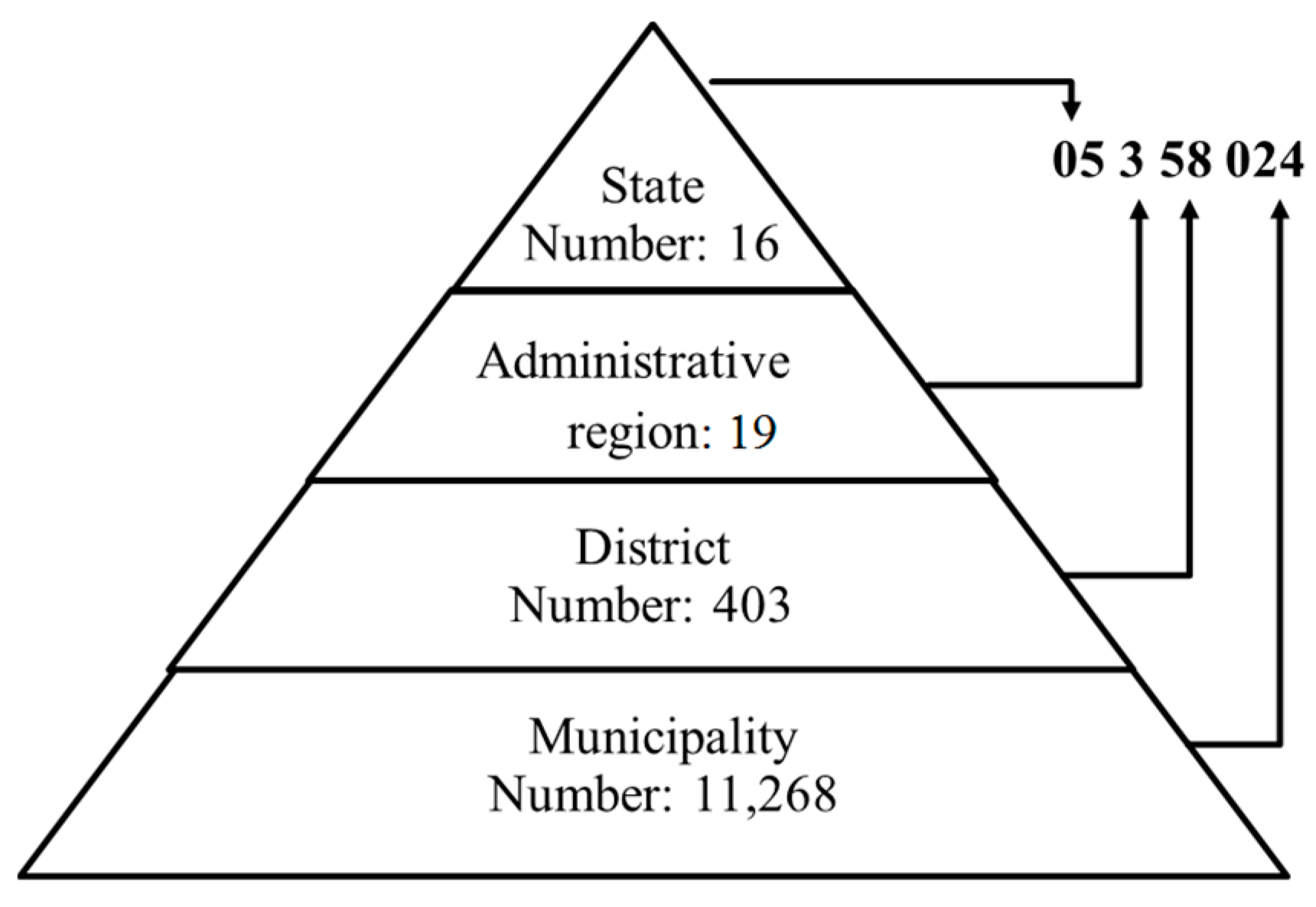
The available data from the TSOs only has a rough spatial resolution, which is not sufficient for detecting the local effects of the grid load. Therefore, a suitable parameter needs to be found in order to achieve a significant spatial resolution with reasonable computational costs. In this paper, the resolution is increased to the municipal level, leading to a subdivision of Germany into 11,268 zones. Each of these municipalities is referenced by the official municipality key (“Amtlicher Gemeindeschluessel”, AGS), which contains information on the federal state (for example, Baden-Württemberg or Bavaria), administrative region (for example, Kassel) and district (for example, Oberbergischer Kreis or Olpe) in which the municipality is located. The structure of the AGS is shown in Figure 3.

To correctly distribute the load over the municipalities, national gross domestic product (GDP) is a good indicator that is also commonly used in the literature [39]. From 1990 to 2012, a linear correlation between GDP and electricity consumption with a correlation coefficient of 0.91 can be discerned [40].

Due to the fact that GDP is only provided for each administrative district, it must be calculated for each municipality. By simplification, GDP correlates with the population in each municipality, meaning that we can divide the district-level GDP by the number of inhabitants of the district. This simplification leads to a different load compared to the real one in municipalities with a higher GDP compared to the average load on the district level and vice versa.

The population of each district can be generated using the district’s aggregated municipalities: Pop = population, Dis = district, Mun = municipality; x_ij = 1 if municipality j is in district i, otherwise x_ij = 0:

$${\mathrm{Pop}}_{\mathrm{Dis},\mathrm{i}}={\displaystyle \sum }_{\mathrm{j}}{\mathrm{Pop}}_{\mathrm{Mun},\mathrm{j}}\times {\mathrm{x}}_{\mathrm{ij}}$$

By dividing the GDP of the district by its population:

$${\mathrm{GDP}}_{\mathrm{per}\mathrm{inhabitant};\mathrm{Dis},\mathrm{i}}=\frac{{\mathrm{GDP}}_{\mathrm{Dis},\mathrm{i}}}{{\mathrm{Pop}}_{\mathrm{Dis},\mathrm{i}}}$$

the GDP for each inhabitant in the district is thereby generated. Now, the GDP per municipality can be calculated as:

$${\mathrm{GDP}}_{\mathrm{Mun},\mathrm{j}}={\mathrm{GDP}}_{\mathrm{per}\mathrm{inhabitant},\mathrm{Dis},\mathrm{i}}\times {\mathrm{Pop}}_{\mathrm{Mun},\mathrm{j}}$$

When the GDP is known for each municipality, the load of each TSO’s region can be transferred from the TSO- to the municipalities-level. The GDP of all municipalities in the TSO area must be aggregated using y_TSO,j = 1 if municipality j is in the TSO area, otherwise y_TSO,j = 0.

$${\mathrm{GDP}}_{\mathrm{TSO}}={\displaystyle \sum }_{\mathrm{j}}{\mathrm{GDP}}_{\mathrm{Mun},\mathrm{j}}\times {\mathrm{y}}_{\mathrm{TSO},\mathrm{j}}$$

Now, for each municipality, an individual load factor can be calculated. This load factor represents the load share of the municipality in the overall load from the TSO:

$${\mathrm{Load}\mathrm{factor}}_{\mathrm{Mun},\mathrm{j}}=\frac{{\mathrm{GDP}}_{\mathrm{Mun},\mathrm{j}}}{{\mathrm{GDP}}_{\mathrm{TSO}}}$$

3.2. Adjustment of Load Factors

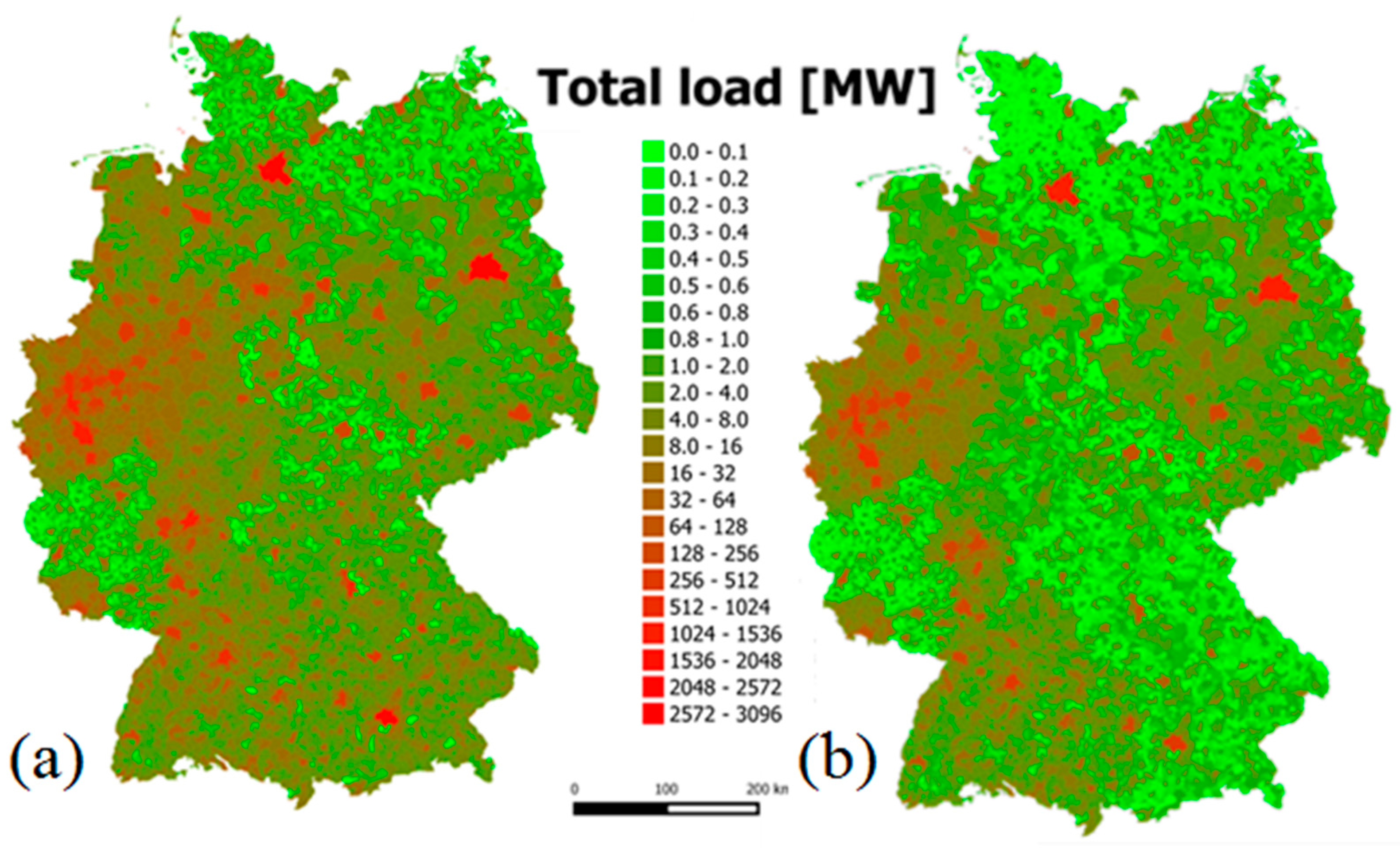
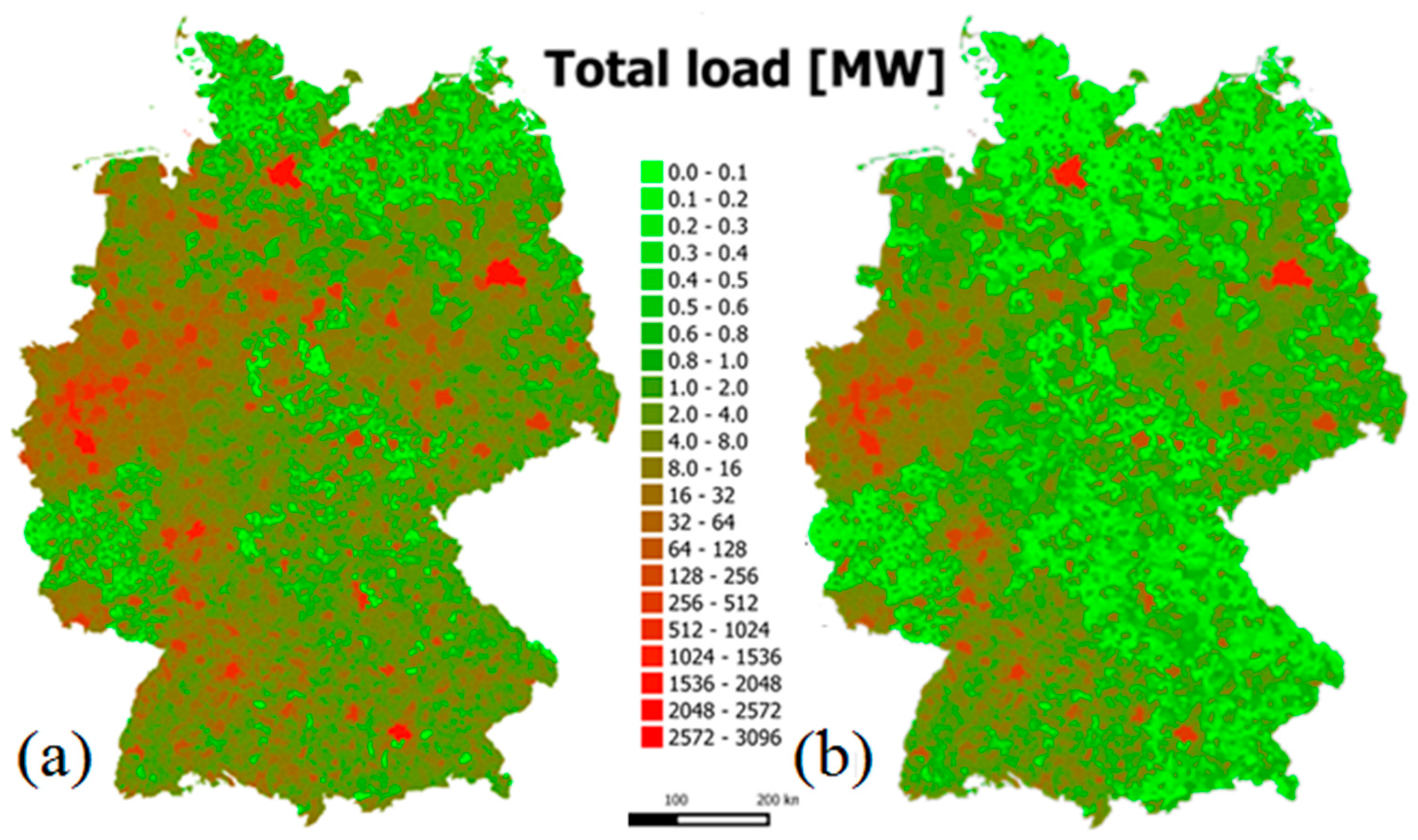
The load factors can be used to visualize the related electrical load in each municipality for each period of time, as shown in Figure 4 for the highest (a) and lowest (b) loads recorded in 2013. To show this value at an hourly resolution, the four quarterly-hour values in this hour were summarized. Figure 4 also shows the major load consumption in the large cities of Berlin ((a) 2701 MW, (b) 1402 MW), Hamburg ((a) 2496 MW, (b) 1296 MW), Munich ((a) 2112 MW, (b) 330 MW) and Stuttgart ((a) 1016 MW, (b) 453 MW). Heavy industry, shown as a high load, in the states of North Rhine-Westphalia (NRW) and Saarland can also be seen. The average load in NRW of ((a) 48.6 MW per municipality and (b) 23.3 MW per municipality) is higher than the German average load per municipality in both cases, namely 6.71 MW (a) and 2.62 MW (b).

To validate the model with existing data at the same resolution was not possible due to the non-existing data. Especially at the distribution level, detailed knowledge of the load is missing. Therefore, to validate the model’s results, the loads it depicts are compared with consumption drawn from statistical data. Due to the fact that statistical data on consumption are only available at the state level and only for a period of one year, the load for each municipality was aggregated at the state level.

Table 3. Comparison: model vs. statistical data in 2010 [37,41,42,43,44,45,46,47,48,49,50,51,52,53,54,55,56].

State 2010	Sum Load Model (TWh)	Consumption Statistical Data (TWh)	Sum Load Model/Consumption Statistical Data (-)
Baden-Württemberg	63.76	72.74	0.88
Bavaria	77.37	82.32	0.94
Berlin	19.18	13.00	1.48
Brandenburg	10.71	13.68	0.78
Bremen	4.36	4.96	0.88
Hamburg	17.72	12.95	1.38
Hessen	41.85	37.26	1.12
Mecklenburg-Western Pomerania	6.73	6.53	1.03
Lower Saxony	37.88	52.94	0.72
North Rhine-Westphalia	123.68	120.37	1.03
Rhineland-Palatinate	25.37	28.17	0.90
Saarland	6.95	7.98	0.87
Saxony	18.09	19.36	0.93
Saxony-Anhalt	9.75	14.69	0.66
Schleswig-Holstein	12.20	11.57	1.05
Thuringia	9.21	12.48	0.74
Sum	484.81	511.00	0.95

shows the difference between the modeled data and that from the statistics for 2010. In 10 of the 16 states, the maximum consumption difference was about 15%. To reduce errors, the load factors were adjusted.

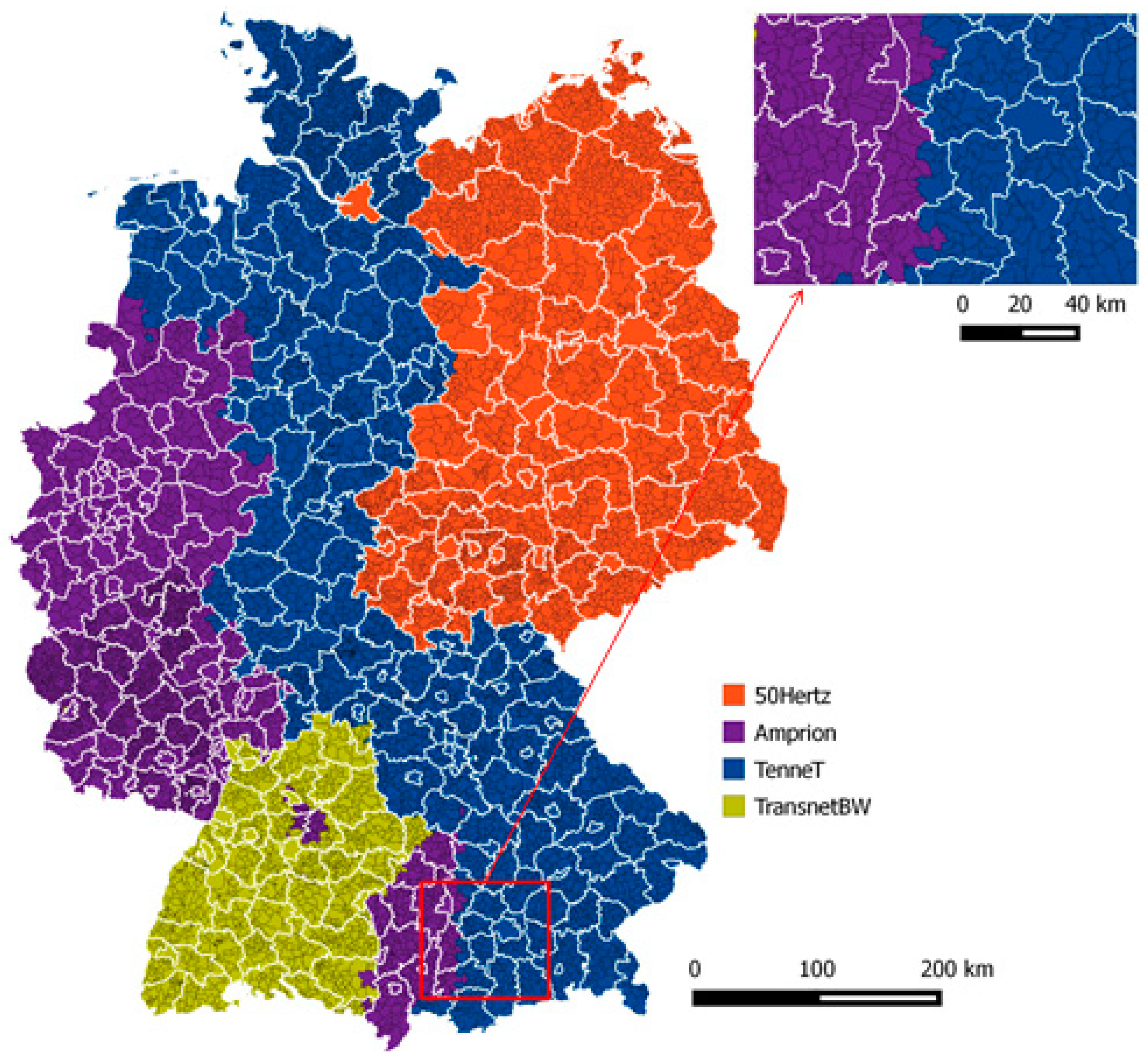
The borders of the states do not necessarily correspond to the borders of the TSOs. Therefore, each state is assigned one or more TSO and its specific share. The shares of the four TSOs in each state were investigated using master data (“Anlagenstammdaten”) from the TSOs.

These master data contain information on nearly all renewable energy sources (RES) in Germany. In addition to other information, the location, state, municipality and TSO are included in these master data. Hence, each municipality with RES can be associated with the corresponding TSO. Municipalities with no RES are associated with the TSO nearest to the municipality. To calculate the share of the TSO in each state, the population of the municipality was divided by the population falling under the TSO. Thus, the population was used instead of the area. In this way, areas with no population, for example forests, were excluded. The results are shown in

Table 4. Share of the TSO in each state in terms of supplied population.

State	50 Hertz (%)	Amprion (%)	TenneT (%)	TransnetBW (%)
Baden-Württemberg		3.75	0.04	96.22
Bavaria		14.35	84.15	1.50
Berlin	100
Brandenburg	100
Bremen			100
Hamburg	100
Hessen		42.28	57.18	0.55
Mecklenburg-Western Pomerania	100
Lower Saxony	0.13	11.46	88.40
North Rhine-Westphalia		91.28	8.72
Rhineland Palatinate		99.97		0.03
Saarland		100
Saxony	100
Saxony-Anhalt	99.39		0.61
Schleswig Holstein			100
Thuringia	100

. Berlin, Brandenburg, Hamburg, Mecklenburg-Western Pomerania, Saxony and Thuringia are in the area of 50 Hertz. In contrast, Amprion, TenneT and TransnetBW hold a share in Baden-Württemberg.

The share of each TSO in the states, as shown in Table 4, the statistical consumption data in Table 3 and the load values in

Table 5. Aggregated load of each TSO for 2010 per quarter-hour.

	50 Hertz	Amprion	TenneT	TransnetBW	Sum
∑Load valueTSO/4	91.4 TWh	190.1 TWh	141.3 TWh	62.1 TWh	484.9 TWh

can now be used to calculate the share of each TSO and each state from the statistical data:

$${\mathrm{Real}}_{\mathrm{TSO}.\mathrm{state}}={\mathrm{Share}}_{\mathrm{TSO}.\mathrm{state}}\times \frac{\mathrm{Stat}.{\mathrm{consumption}}_{\mathrm{state}}}{{\displaystyle \sum }{\mathrm{Load}\mathrm{value}}_{\mathrm{TSO}}/4}$$

The load value of the TSO must then be divided by 4, as it is the sum of quarterly-hour values.

Optimally, the sum of the shares of each TSO should be 100% for the quotient of statistical data of consumption and load value. However, the “real” statistical data shares of 50 Hertz, TenneT and TransnetBW (see

Table 6. Comparison between the modeled data, real consumption data and real normalized consumption data in 2010.

State	50 Hertz				Amprion				TenneT				TransnetBW
	Model (%)	Real (%)	Real Normalized (%)	Variance (%)	Model (%)	Real (%)	Real Normalized (%)	Variance (%)	Model (%)	Real (%)	Real Normalized (%)	Variance (%)	Model (%)	Real (%)	Real Normalized (%)	Variance (%)
Baden-Württemberg					1.47	1.43	1.50	−0.03	0.01	0.02	0.02	0.00	98.21	112.78	97.99	0.22
Bavaria					6.89	6.21	6.48	0.41	44.82	49.04	42.11	2.71	1.54	1.99	1.73	−0.18
Berlin	20.99	14.23	14.03	6.96
Brandenburg	11.72	14.97	14.76	−3.04
Bremen									3.09	3.51	3.01	0.07
Hamburg	19.39	14.18	13.98	5.41
Hessen					10.32	8.29	8.64	1.68	15.63	15.08	12.95	2.68	0.24	0.33	0.28	−0.05
Mecklenburg-Western Pomerania	7.36	7.15	7.05	0.32
Lower Saxony	0.05	0.08	0.08	−0.03	3.09	3.19	3.33	−0.24	22.63	33.13	28.45	−5.82
North Rhine-Westphalia					61.24	57.80	60.24	0.99	5.14	7.43	6.38	−1.24
Rhineland Palatinate					13.34	14.81	15.44	−2.10
Saarland					3.66	4.20	4.38	−0.72
Saxony	19.79	21.19	20.89	−1.10
Saxony-Anhalt	10.61	15.98	15.75	−5.14					0.04	0.06	0.05	−0.02
Schleswig Holstein									8.64	8.19	7.03	1.61
Thuringia	10.08	13.66	13.47	−3.39
Sum	100.0	101.4	100.0	0	100.0	95.9	100.0	0	100.0	116.5	100.0	0	100.0	115.1	100.0	0

) actually add up to 101.4%, 116.5% and 115.1%, respectively. These values are therefore too high, while the share of Amprion, at 95.94%, is too low. These deviations result from the different values for aggregated load and consumption (see Table 3 and Table 5), yet the statistical consumption was 5% higher than the modeled data. To counteract this problem, the statistical data was normalized as follows:

$${\mathrm{Real}\mathrm{normalized}}_{\mathrm{TSO}.\mathrm{State}}=\frac{{\mathrm{Real}}_{\mathrm{TSO}.\mathrm{State}}}{{{\displaystyle \sum }}_{\mathrm{State}}{\mathrm{Real}}_{\mathrm{TSO}.\mathrm{State}}}$$

The result is shown in Table 6, in the column labeled “real normed”. In order to compare the modeled and real normed data, the variance between them is calculated in Table 6. For example, according to statistical data, the share of 50 Hertz in Berlin is 14.23%. According to the real normalized, this share is 14.03%, which is 6.96% lower than the modeled data, at 20.99%.

The adjustment factor is:

$${\mathrm{Adjustment}\mathrm{factor}}_{\mathrm{TSO}.\mathrm{State}}=\frac{{\mathrm{Real}\mathrm{normalized}}_{\mathrm{TSO}.\mathrm{State}}}{{\mathrm{Model}}_{\mathrm{TSO}.\mathrm{State}}}$$

Table 7. The adjustment factors for each state.

State	50 Hertz (%)	Amprion (%)	TenneT (%)	TransnetBW (%)
Baden-Württemberg		101.86	107.11	99.76
Bavaria		94.06	93.95	111.74
Berlin	66.83
Brandenburg	125.95
Bremen			97.61
Hamburg	72.08
Hessen		83.72	82.83	119.92
Mecklenburg-Western Pomerania	95.70
Lower Saxony	164.81	107.72	125.73
North Rhine-Westphalia		98.38	124.10
Rhineland Palatinate		115.73		242.71
Saarland		119.62
Saxony	105.54
Saxony-Anhalt	148.42		145.45
Schleswig Holstein			81.39
Thuringia	133.59

shows the factors calculated for each state. To generate the adjusted load factor, the normal load factor was multiplied by the adjustment factors from Table 7. The computational steps are now explained using the example of 50 Hertz and Berlin. The “Real_TSO,State” was determined by multiplying the share value of 50 Hertz in Berlin, taken from Table 4, by the quotient of the consumption data for Berlin, taken from Table 3, “Consumption statistic data”, divided by the aggregated load of “50 Hertz”, taken from Table 5. In other words:

$${\mathrm{Real}}_{50\mathrm{Hertz}.\mathrm{Berlin}}=100\%\times \frac{13.0\mathrm{TWh}}{91.4\mathrm{TWh}}=14.23\%$$

This calculation was performed for every state and TSO. Then, the values for “Real_TSO,State” were added up for each TSO. The sums for each TSO are given in the last row of Table 6 in the column, “Real”. The “Real_TSO,State” values can be normalized with these sums:

$${\mathrm{Real}\mathrm{normalized}}_{50\mathrm{Hertz}.\mathrm{Berlin}}=\frac{14.23\%}{101.4\%}=14.03\%$$

The adjustment factor for Berlin can then be calculated using the values in Table 6 in the columns “Real normalized” and “Model”. The adjustment factor is given in Table 7.

$${\mathrm{Adjusting}\mathrm{factor}}_{50\mathrm{Hertz}.\mathrm{Berlin}}=\frac{14.03}{20.99}=66.8\%$$

Due to the fact that the load from the TSOs only covers about 91% of the total load (compare Table 2), an additional steady load will in the end be applied to the model according to the methodology from Agora Energiewende ([57], p. 5). For the year 2013 this steady load is for example 7.4 GW, which will be divided up by the average of the yearly load to the load at the municipality level.

4. Results

The load situation with the adjusted load factors for the highest (5 December 2013, 18:00) and lowest (2 June 2013, 07:00) electrical load in 2013 can be seen in Figure 5, which adds up to 76 and 30 GW. This can be compared to the unadjusted load factors in Figure 4. In the case of the highest load, for example, the load in Berlin sinks from 2.701 MW to 1.805 MW and, in Munich, from 2.112 MW to 1.985 MW. The share of 50 Hertz in Berlin is thus transferred to Brandenburg, Saxony, Saxony-Anhalt and Thuringia.

After adjustment, Munich is the community with the highest load at the high-load time. The loads in Saarbruecken and Hannover, for example, increase from 246 MW to 294 MW and from 511 MW to 642 MW, respectively. At the lowest load time, Berlin has the highest load at 973 MW. This represents a change of about 429 MW compared to the unadjusted load of 1.402 MW.

Figure 6 gives insight into the level of detail for our model. The black dots indicate the location of energy-intensive industries in Germany [58]. An overall match between municipalities with a high electrical load and the location of energy-intensive industry is also visible. The magnification in Figure 6 shows the locations of energy-intensive industry in more detail. Obviously, municipalities with energy-intensive industry have a higher electric load than neighboring municipalities without such industry.

Figure 7 shows the electrical load with the adjusted load factors and the additional steady load with 7.4 GW for 2013 for the highest (5 December 2013, 18:00) and lowest (2 June 2013, 07:00) load, which amounts to 83 and 37 GW.

5. Conclusions

This paper demonstrates that vertical grid load cannot be used to model electrical load. Since the feed-in into the distribution grid is not properly accounted for by the vertical grid load, the amount of VRES that is usually fed into the distribution grid is always miscalculated. Therefore, we recommend using the total load published by the TSOs. This total load can be extrapolated down from the TSO to the municipality level using the indicators of GDP and the population of each municipality. This yields an initial picture of the electrical load in municipalities in Germany. When the modeled data was compared with statistical electricity consumption at the state level, an average deviation of 17% was revealed and an adjustment factor for each state was thereby calculated. Multiplying this adjustment factor by the load factor yielded the adjusted load factor, which accurately reflects the load in each municipality. This approach also depicts the locations of energy-intensive industry in Germany. When the adjustment factor was applied, the maximum deviation was reduced from 17% to 6.96%. The methodology developed in this paper relies strongly on open source data. Therefore, the approach can also be applied in different countries or used directly for Germany with the described methodology. Furthermore, the electricity load model has a high spatial (municipalities-level) and timely (up to quarter-hours) resolution. A lower resolution can be easily applied by adding either municipalities to districts or quarter-hours to hours.