1. Introduction
Spectral decomposition technology can improve the level of seismic data processing and interpretation, which is helpful to describe reservoir shape and change rules [
1]. Spectrum decomposition mainly has a short-time Fourier transform, wavelet transform, matching pursuit algorithm and Hilbert–Huang transform (HHT) [
2,
3]. Short-time Fourier transforms effectively improves the time resolution, but also reduces the frequency resolution. Wavelet transform can provide high frequency resolution in low frequency bands and high time resolution in high frequency bands, but there is a problem in the selection of wavelet function. The matching pursuit algorithm provides better temporal resolution and frequency resolution, but the computational complexity is huge. Hilbert–Huang transform (HHT) provides a popular data-driven method to analyze nonlinear and non-stationary data [
4]. HHT can process any signal without prior knowledge and is not be limited by the Heisenberg uncertainty principle. However, HHT also has some disadvantages, such as mode mixing, endpoint effect, instantaneous frequency error and so on [
5]. The key part of the method is the empirical mode decomposition (EMD), which can decompose the signal into a finite number of intrinsic mode functions (IMF) in the temporal domain, with each IMF being a narrow-band signal [
6,
7]. However, the EMD method can not guarantee orthogonality between the decomposed IMF and aliasing between IMFs, which is unfavorable for seismic data analysis and may lead to an incorrect interpretation [
5,
8]. The mode mixing problem of EMD will be described in detail in
Section 2. Wu et al. proposed the improved EMD decomposition method, namely the ensemble empirical mode decomposition, which alleviates the mode mixing problem to a certain extent, but its computational complexity is relatively large and there is a large error after signal reconstruction [
9].
HHT has been used in geophysical prospecting since it was firstly proposed. Battista et al. used the EMD with signals of seismic reflection data [
10]. Bekara et al. proposed a new filtering technique to deal with the random noise based on EMD [
11]. Cai et al. applied HHT to the analysis of magneto telluric data and obtained some meaningful geological information [
8]. Huang et al. introduced the extraction method of seismic attributes based on HHT [
12]. Zhou et al. demonstrated the new insights of EMD and HHT which can be used with seismic reflection data [
13]. Xue et al. used the three EMD-based analysis methods to perform a comparative study on hydrocarbon detection [
14]. Han et al. used EMD for seismic time-frequency analysis [
15]. Wang et al. proposed the improved HHT algorithm, which can effectively overcome the shortage of HHT [
5]. Xue et al. studied the EMD-based highlight volume methods, which can be used for hydrocarbon detection [
16]. Gairola et al. used HHT to analyze the heterogeneity of geophysical well-log data [
17]. These articles mainly use EMD to solve the problem of processing and interpretation in seismic data; the disadvantages of EMD decomposition are considered inadequate.
In this paper, we analyze the mode mixing problems and introduce noncontact measurement and detection of instantaneous attributes of seismic signals using complementary ensemble empirical mode decomposition (CEEMD). The synthesis signals are decomposed by EMD and CEEMD; the results indicate that CEEMD can effectively solve the mode mixing problems of EMD. The decomposed results of the synthetic seismic record show that CEEMD has a better ability to decompose seismic signals. Based on the actual seismic data, the composition results of CEEMD show that the second intrinsic mode functions (IMF2) profile contains main reflectors, and the instantaneous seismic attributes extracted from the decomposed IMF2 profile are helpful to effectively identify the undulations of the top interfaces of limestone. The contribution of this paper is hence that the instantaneous seismic can be accurately detected by the proposed CEEMD method.
2. The Proposed Method
Based on the analyses of possible reasons of mode mixing problems, Yeh et al. have put forward the CEEMD algorithm for decomposition [
18]. Based on the use of several groups of auxiliary positive and negative white noise, the CEEMD could better remove residual noise during signal reconstruction and has higher calculation efficiency, thus effectively solving mode mixing problems during EMD decomposition process. Colominas et al. proposed a new improved CEEMD; the new method was used for artificial signals and real biomedical signals [
19]. The improvements of the CEEMD method have been achieved through the application of correlation theory [
20,
21,
22,
23,
24]. The main steps of the CEEMD are as follows:
(1) Firstly,
n groups of white noise (positive and negative auxiliary) are added into the signal to generate two sets of signals, as follows:
In the formula, refers to the original signal, is the auxiliary noise, and and are new generated signals. 2n signals are obtained, and can be determined by the residual between the decomposed signal and the original signal. While the residual is less than the threshold, the operation of adding white noise will stop.
(2) The EMD is applied to each signal in the set to get a set of IMF components in which the jth IMF component of the ith signal could be expressed as .
(3) The added noise could be removed by calculating the sum and averages of the components; the results are as follows:
2.1. Mode Mixing Problem
This paper is not going to cover the basic principles of HHT which have been introduced in much of the literature [
1,
2,
3,
4,
5,
6,
7,
8,
9,
10,
11,
12,
13,
14,
15,
16]. We will focus only on mode mixing problems of the EMD method in HHT.
As a data-driven and adaptive decomposition method, the EMD method aims to decompose the complex signals into IMF. The principle of EMD is as follows: firstly, we extract IMF1, and then the original signal minus the IMF1, which we can see as a new sequence. We then decompose this new sequence to get IMF2, IMF3, etc., until the residual sequence is a monotone sequence, and the residual sequence is the residual component. The mode mixing problems arise as a result of the same IMF containing components with different scales, which directly cause a lack of physical significance and is not useful for signals analysis and interpretation.
The following signals are utilized to present mode mixing problems.
is obtained by the stacking of
and
, where
is calculated by a tractable sine function over the whole period, and
is obtained by two frequency cosine functions, as follows:
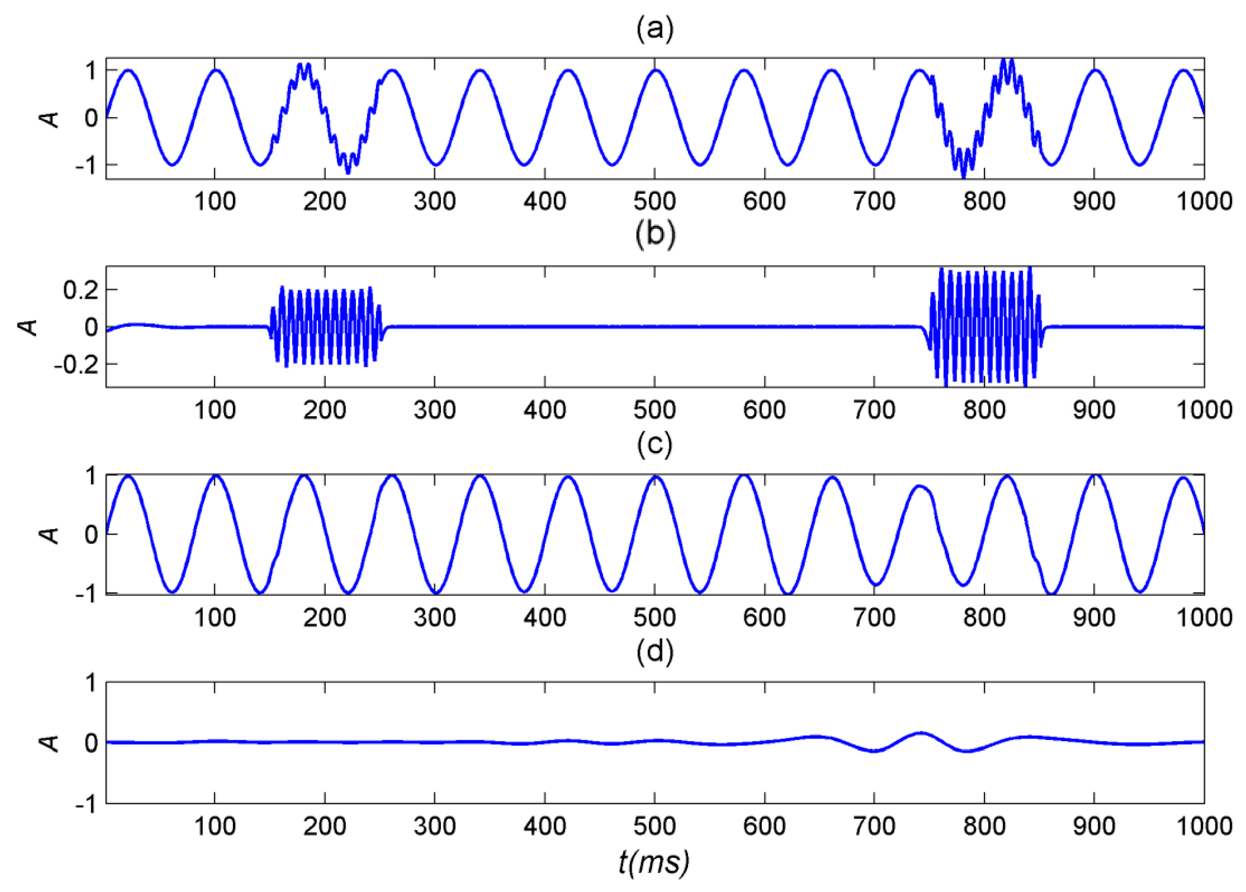
The EMD is used for signal decomposition. As shown in
Figure 1, due to the high frequency intermittent cosine signals, the intermittent high frequency signals in IMF1 could not be properly separated.
Intermittent high frequency signals lead to mode mixing problems in the results of EMD. The high frequency components and other low frequency components are incorrectly included in IMF1 and very different oscillations could be found in the same mode. As the decomposition proceeds, such mode errors will continue. The mode mixing problems cause the original signals to be unable to be reasonably decomposed, which have serious effects on EMD’s subsequent decomposition and destroys the physical meaning of IMF.
2.2. The Decomposed Results of CEEMD
Figure 2 shows the decomposition results of CEEMD which are verified by the signals in formula (1). In
Figure 2, high frequency signals are decomposed into mode components which are consistent with the original signals. The results show that CEEMD could effectively solve the problem of mode mixing by adding groups of white noise (positive and negative auxiliary) and has better decomposition effects.
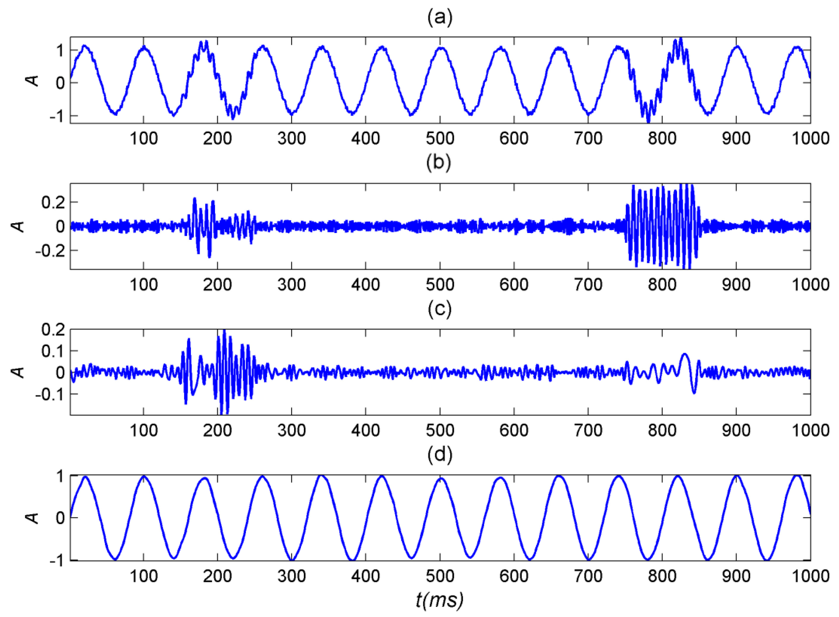
2.3. Anti-Noise Ability Test of CEEMD
To verify the anti-noise ability of CEEMD, 15 percent of white Gaussian noise (with mean 0 and variance 1) is added to the above signals and then decomposed by CEEMD.
Figure 3 shows the results. After decomposition, IMF1’s corresponding amplitude value is 0.3 of a high frequency signal and IMF2’s corresponding amplitude value is 0.2 of a high frequency signal. IMF3’s corresponding signal is a sinusoidal signal. The decomposition results show that CEEMD could not only overcome the problem of mode mixing but also has better anti-noise ability.
The above test results show that CEEMD has the following advantages:
- (1)
The results of CEEMD decomposition are closer to actual waveform components while the results of EMD decomposition deviate from actual signals. The results show that CEEMD could effectively solve mode mixing problems.
- (2)
CEEMD could correctly and accurately display the positions of high frequency transient signals. CEEMD has a better anti-noise ability. It could guarantee the decomposition effects at higher noise levels.
2.4. Instantaneous Seismic Attributes
Instantaneous seismic attributes are being widely used in seismic prospecting [
25,
26,
27], mainly including instantaneous amplitude, instantaneous frequency and instantaneous phase. Tanner et al. firstly applied the analytic signal to construct the seismic trace to get instantaneous attributes [
28]. Robertson et al. applied complex seismic trace analysis method for thin layer interpretation [
29]. Barnes studied calculation methods of instantaneous frequency attribute and instantaneous bandwidth attribute, put forward the concept of local weighted averaging of instantaneous seismic attributes and further promoted the application of instantaneous seismic attributes [
30,
31].
In the following, the seismic signal is assumed to be
c(
t), and the corresponding “analytical signal” is as follows:
where
is the Hilbert transform of
c(
t), and
. Based on the analytic signals, the instantaneous amplitude attribute is as follows:
Namely, as the square root of the total energy of the real and imaginary parts of the analytic signal, where
is a measure of reflected intensity. It mainly reflects the changes in energy and could highlight special strata changes. The instantaneous phase attribute is defined as follows:
The instantaneous phase offers a measure of the continuity of events on a seismic section. When the seismic waves propagate through anisotropic medium, the phase is continuous. When the seismic waves propagate through abnormal medium, significant changes of the phase could be observed in the abnormal position and the phase discontinuity could be observed in the profile. Therefore, the instantaneous phase could be utilized to identify the surface undulation of a geologic body. Lastly, the instantaneous frequency attribute is defined as follows:
where
is the instantaneous frequency attribute and
T is the signal sampling period. When seismic waves pass through different medium interfaces, the frequency will change remarkably. The instantaneous frequency attribute could show the lithological changes of strata and is useful to identify strata.
For the same strata, if the above three instantaneous attributes change significantly at the same location, this could maybe reflect the presence of anomalies. Therefore, the three kinds of instantaneous attributes could be utilized for comparative or joint analysis of seismic stratigraphic interpretation.
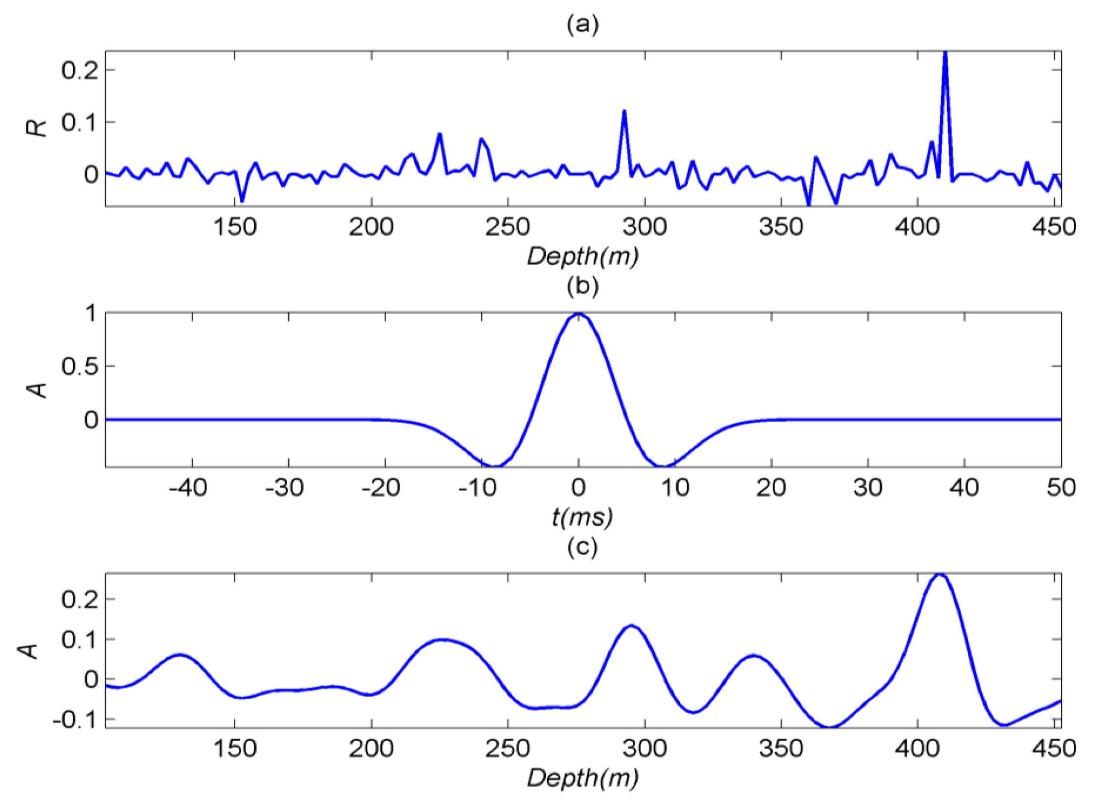
3. The Decomposed Results of Synthetic Seismic Record
We use the logging data from the Ordos Basin of Inner Mongolia for the synthetic record.
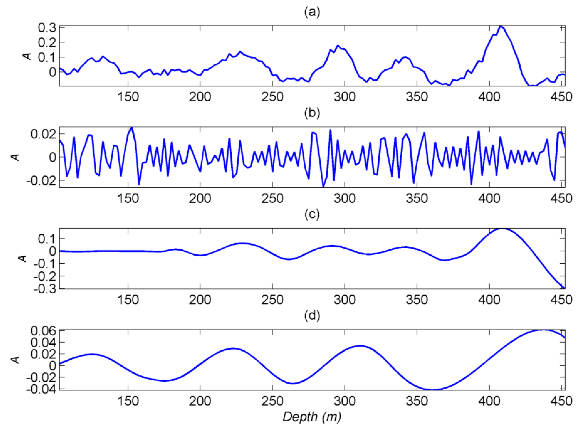
Figure 4a shows the reflection coefficient calculated from the acoustic velocity and density of the logging data.
Figure 4b shows the Ricker wavelet with a frequency of 45 Hz and a length of 100 ms.
Figure 4c is the synthetic record calculated by the deconvolution of reflection coefficient and Ricker wavelet.
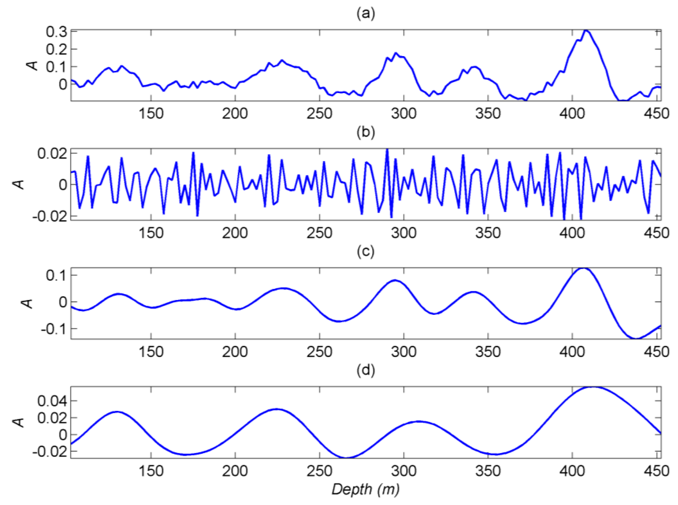
The EMD and CEEMD are used for synthetic seismic record decomposition, as shown in
Figure 5 and
Figure 6, respectively.
In order to test the decomposition ability of CEEMD in the synthetic seismic record, 15 percent of white Gaussian noise (with mean 0 and variance 1) is added to the above signals and then decomposed by EMD and CEEMD, as shown in
Figure 5 and
Figure 6, respectively.
By contrast analysis,
Figure 5 and
Figure 6 shows that IMF1 which was decomposed by EMD and CEEMD is the noise component, IMF2 is the main component of synthetic seismic record, and IMF3 reflects the overall changes trend of synthetic seismic record. The correlation coefficients of IMF1 and noise, IMF2 and synthetic seismic record without noise are calculated respectively, the results are shown in
Table 1, which shows that the CEEMD method has good decomposition ability for synthetic seismic records, and the correlation coefficients of IMF1 and noise, IMF2 and synthetic seismic record without noise are 0.8764 and 0.9201, respectively. The decomposition results are much better than that of EMD.
The decomposition results of synthetic seismic record show that CEEMD has a better ability to decompose seismic signals, where in IMF1 mainly includes noise components while IMF2 is the main component of seismic signals and IMF3 reflects the overall changes trend of seismic signals.
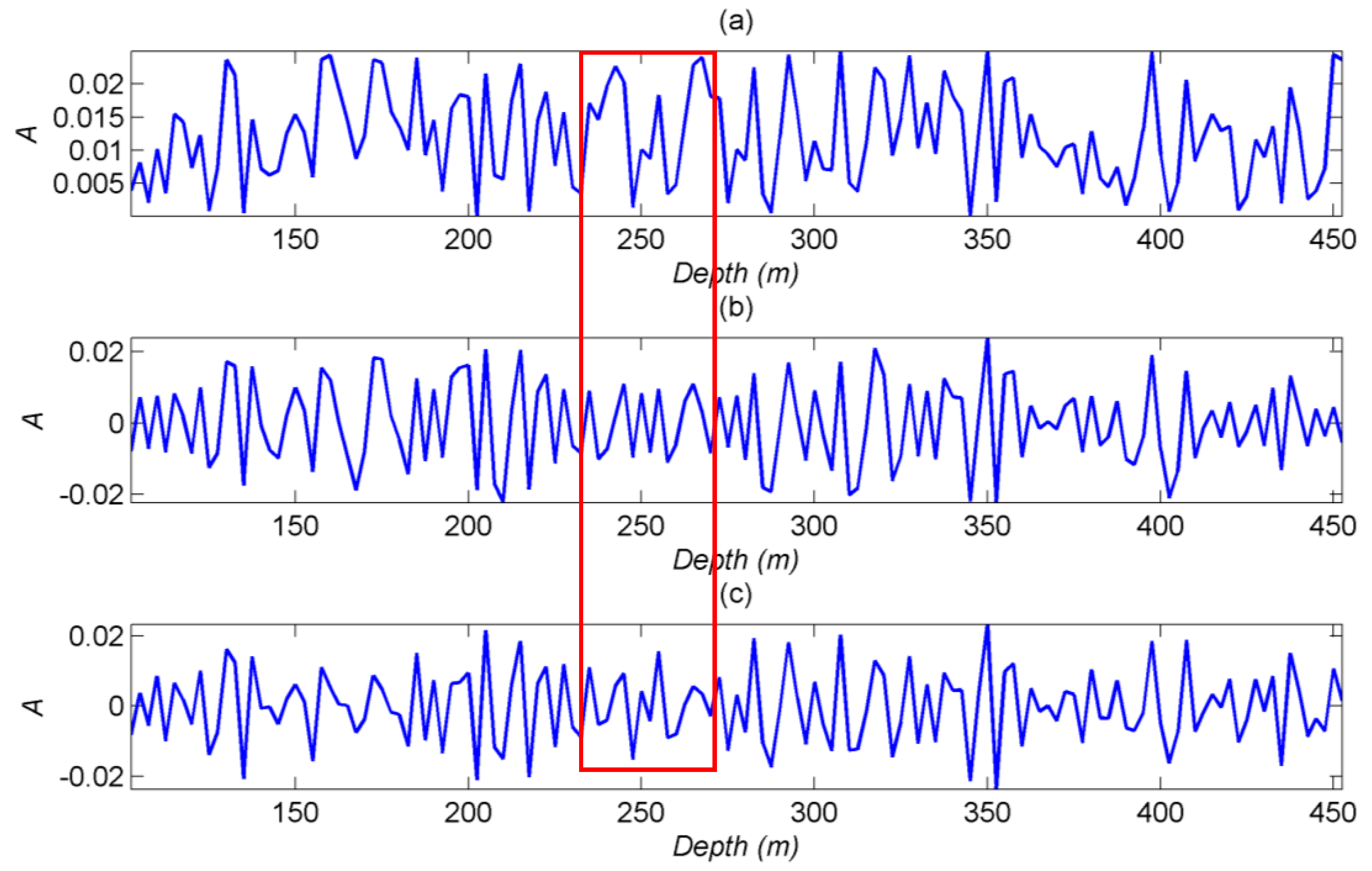
Figure 7 is the white Gaussian noise and IMF1 calculated by the EMD and CEEMD. The IMF1 decomposed by the two methods has basically the same trend as the noise signal.
Table 1 shows that the correlation coefficients of noise and IMF1 calculated by the EMD, noise and IMF1 calculated by the CEEMD are 0.7367 and 0.8764, respectively. The area in the red box of the
Figure 7 shows that the CEEMD has better decomposition effect on white Gaussian noise.
The decomposition results of synthetic seismic record show that CEEMD has a better ability to decompose seismic signals, in which IMF1 mainly includes noise components, while IMF2 is the main component of seismic signals and IMF3 reflects the overall changes trend of seismic signals.
4. Case Study
Since it is always important to evaluate techniques using real-world data, in this paper, real-world seismic data is used to verify the proposed detection method. Most coal-bearing strata belong to the permo-carboniferous system in China. The existence of limestone in the Taiyuan Formation as well as the Ordovician limestone aquifer poses a great security to deep coal mining. With the increasing of mining depth, it is very necessary to investigate the distribution of limestone to ensure the safety production of coal mine [
32,
33].
The present case study is focused on the Ordos Basin of Inner Mongolia. The coal-bearing strata are consisted of carboniferous Taiyuan formation and the Lower Permian Shanxi Formation. Based on the existing drilling data, the distance between the 9# coal seam and the top interface of Ordovician limestone is only 30 m. As the mining of the main coal seam continues, the threat from Ordovician limestone water is increasing. Therefore, it is urgent to identify the undulation of Ordovician limestone top interface. In order to track the horizon of the 9# coal, we use the synthetic record based on velocity and density data [
34] of well logging, which is shown in
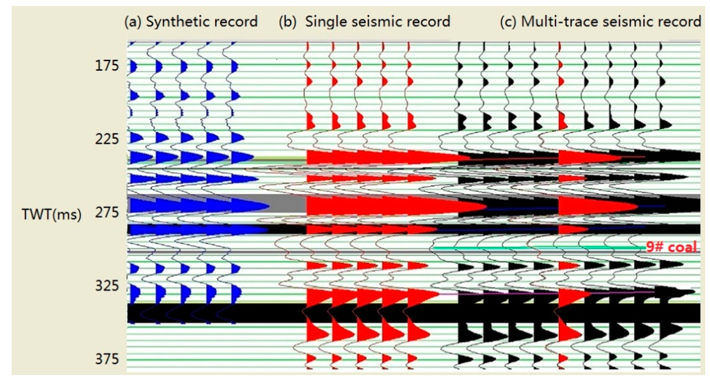
Figure 8.
Figure 8a is the synthetic record,
Figure 8b is the single seismic record comes from
Figure 8c and
Figure 8c is the multi-trace seismic record of real-world data.
Figure 8 shows that the synthetic record and the seismic record have good consistency, the correlation coefficient is as high as 0.83, which can guide us to track the horizon of 9# coal.
The real-world data are acquired by the seismic exploration method. The main parameters of acquisition are as follows: bin of 5 m (Inline) × 5 m (Crossline); fold number of eight times (Inline) × eight times (Crossline); receiving 80 traces/line × 16 lines; trace interval is 10 m; shot interval is 10 m; the interval of receiving lines is 50 m; the interval of the shot lines is 50 m; minimum offset is 7.07 m, maximum offset is 559 m; and the signal sampling period is 1 ms. Then, real-world data are processed and interpreted, and we obtain post-stack 3D seismic data.
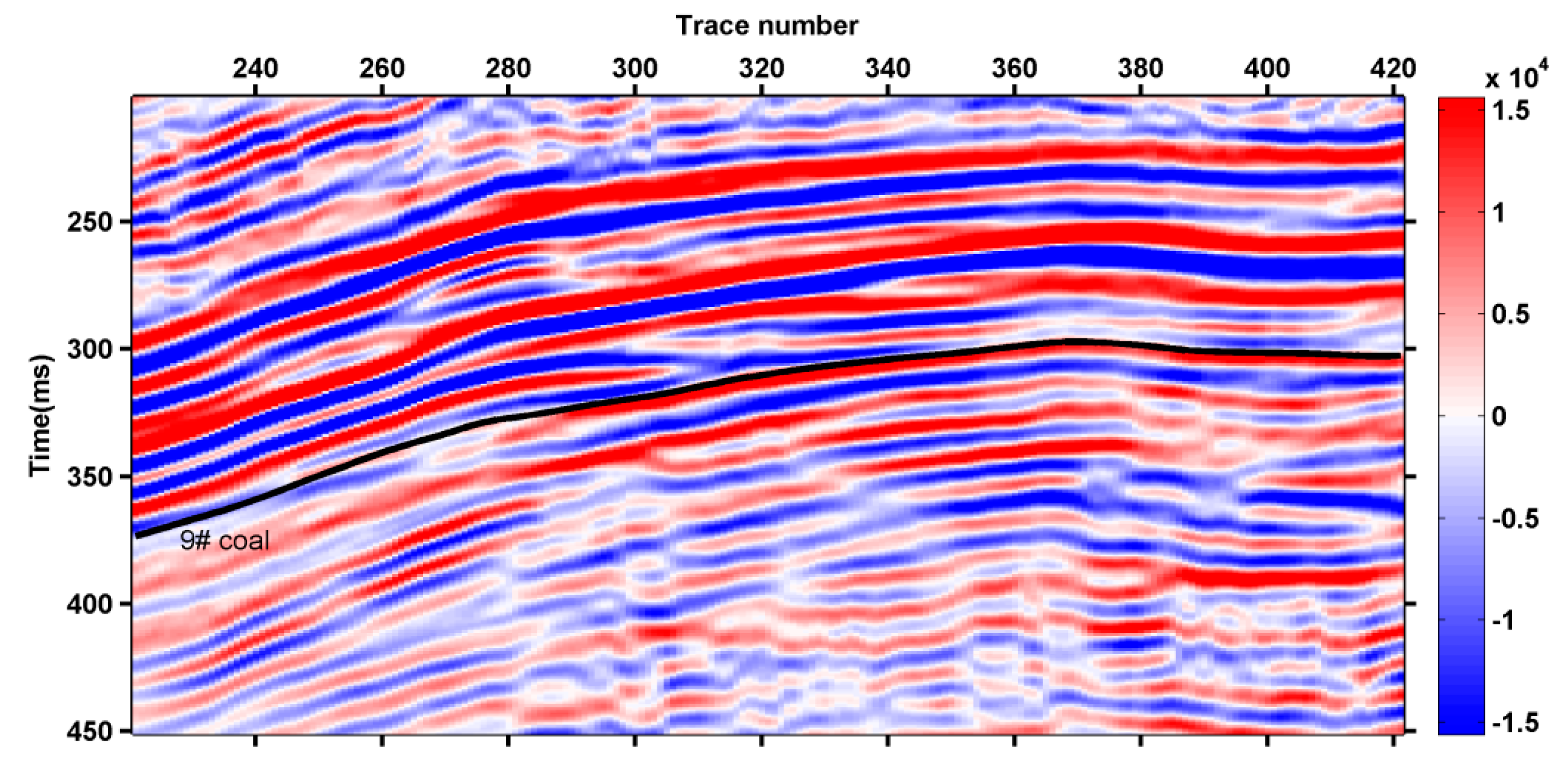
Figure 9 is the original seismic section of this area, which is located at Crossline 485; the horizon of the 9# coal can be tracked by the guide of synthetic record of
Figure 8. As shown in
Figure 9, the 9# coal is a slowly undulating horizon with a tendency towards “west low and east high”.
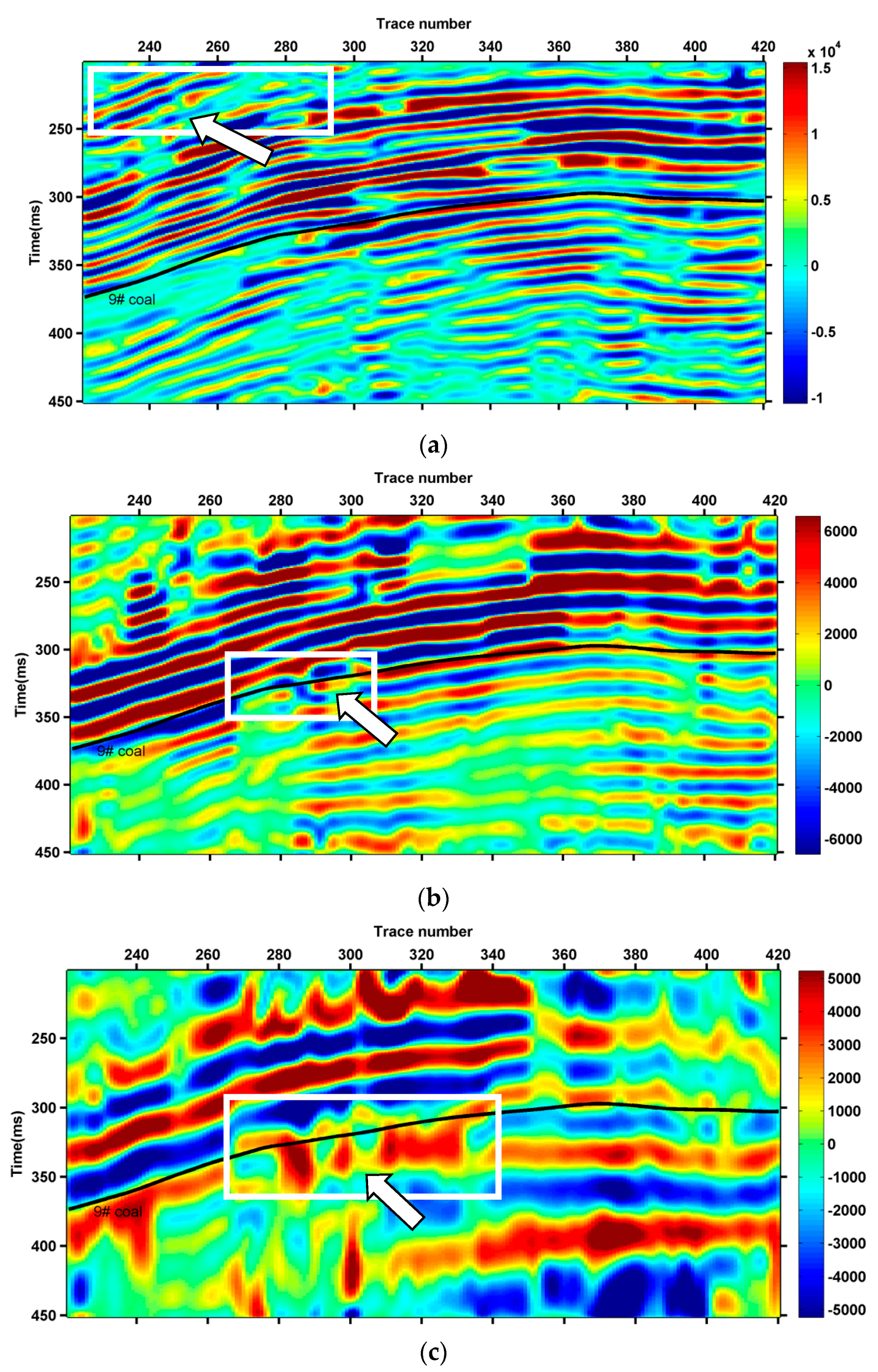
The EMD and CEEMD are utilized to extract IMF components of seismic data in each trace from the original seismic section to form IMF component profile, as shown in
Figure 10 and
Figure 11. In
Figure 10, IMF1 reflects the high frequency information in the seismic data, but “burr” phenomenon, as shown in the white box, the position of the white arrow, which could be found at the top right corner because of the mode mixing problem. IMF2 presents main seismic reflectors, but some events lack details and make the boundary location difficult, as shown in the white box. IMF3 shows blurred seismic reflectors with poor resolution ratio, indicating that the reflection energy is weak at the time scale in seismic data, as shown in the white box.
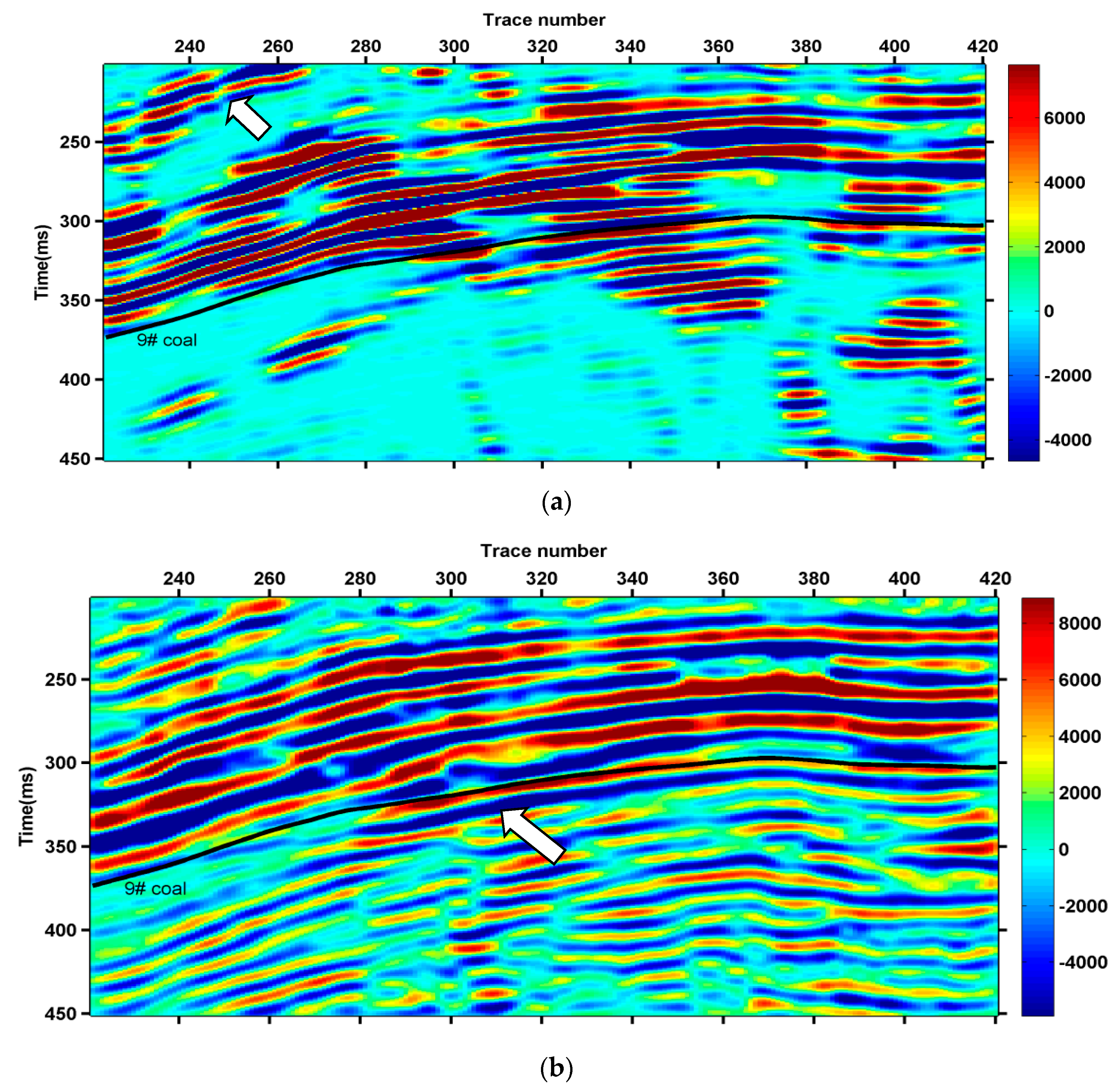
Figure 11 illustrates the decomposition results of CEEMD. It is shown that IMF1 profile mainly reflects high frequency component information. The addition of random white noise effectively overcomes the problem of mode mixing problem and reduces the “burr” phenomenon greatly, such as the position of the white arrow. IMF2 profile contains main seismic reflectors. The events have higher clarity and better continuity and could display strata forms more accurately. IMF3 mainly contains low frequency information. The events of main reflectors are become more clearly and accurately than that of EMD decomposition results.
The comparative analysis of EMD decomposition results and CEEMD decomposition results shows that the latter could better and accurately reflect basic forms of the strata. IMF2 contains main reflectors and has clearer events and better continuity. Therefore, the IMF2 profile based on CEEMD could be utilized for extraction and analysis of instantaneous seismic attributes.
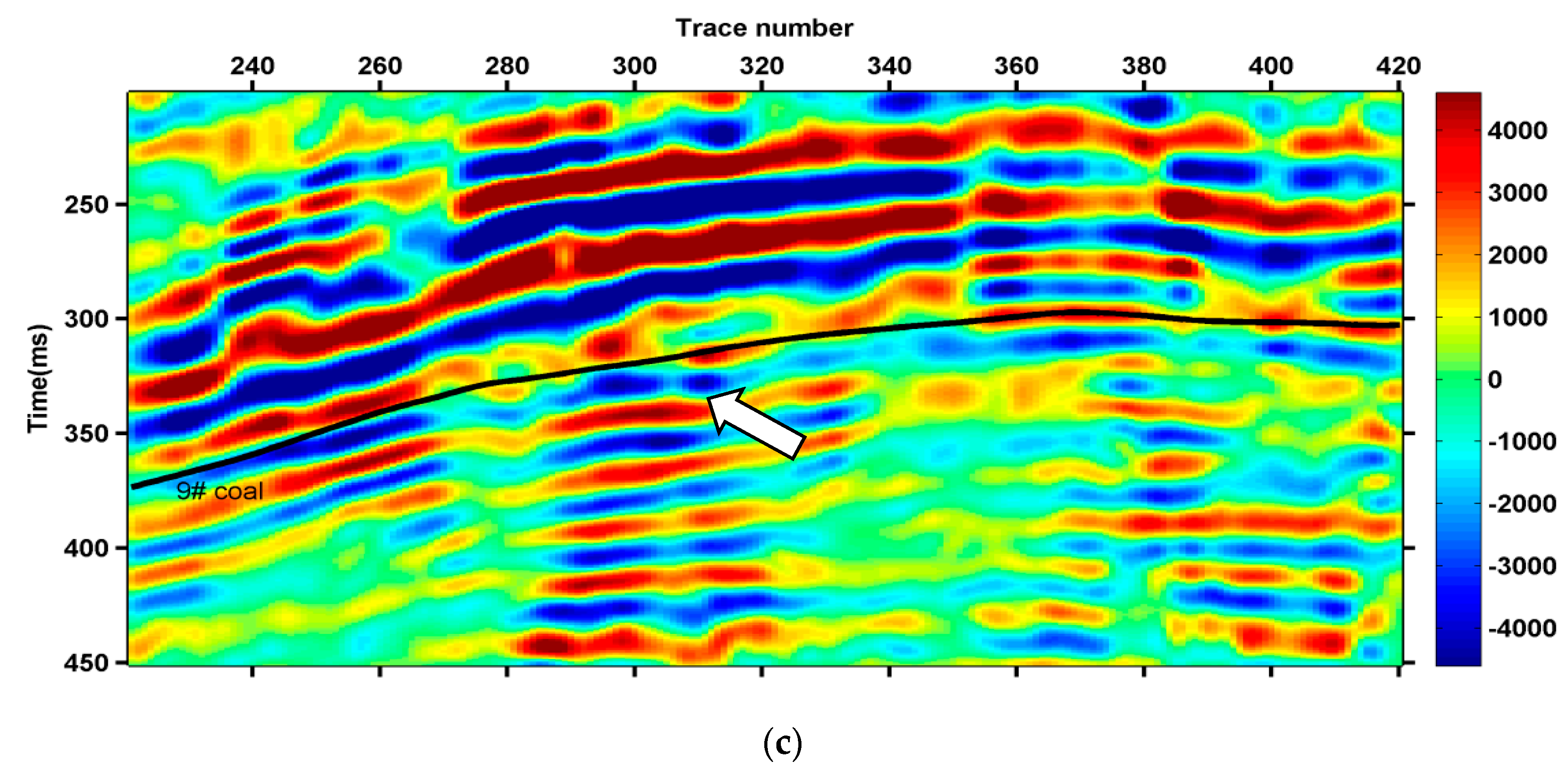
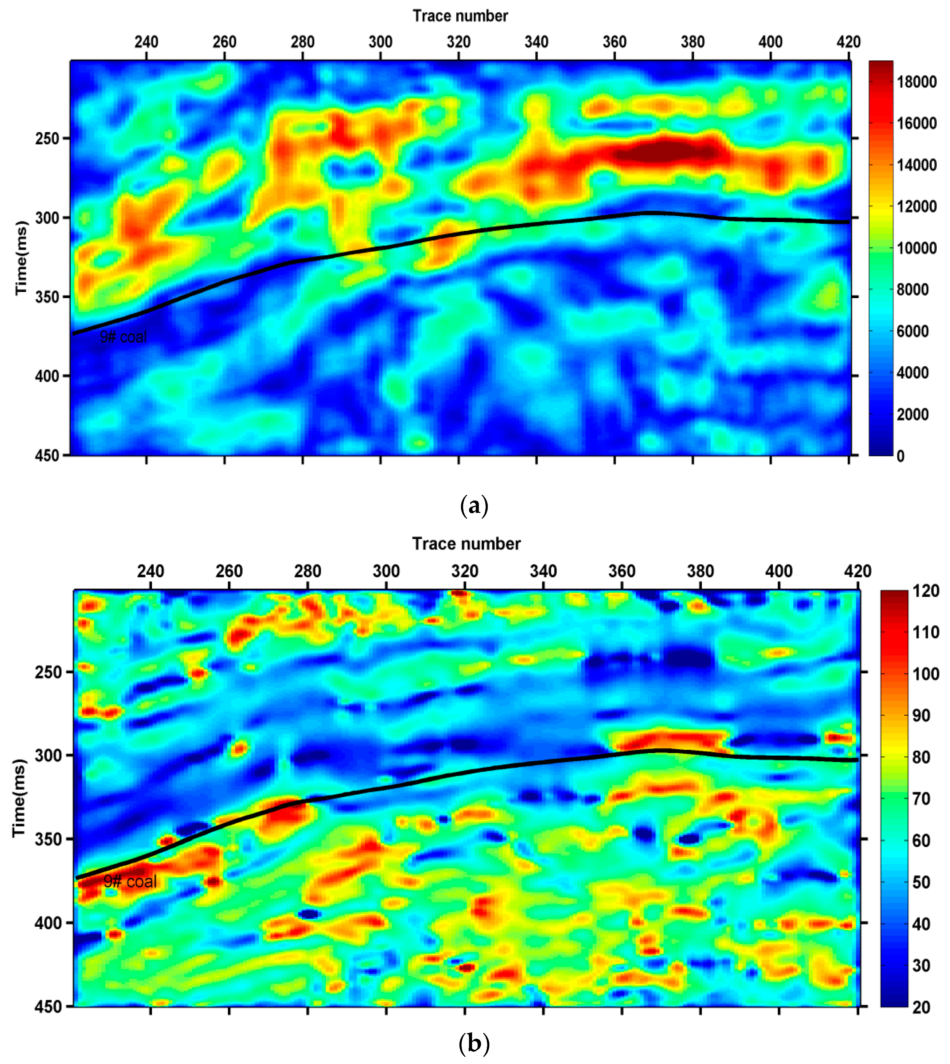
In
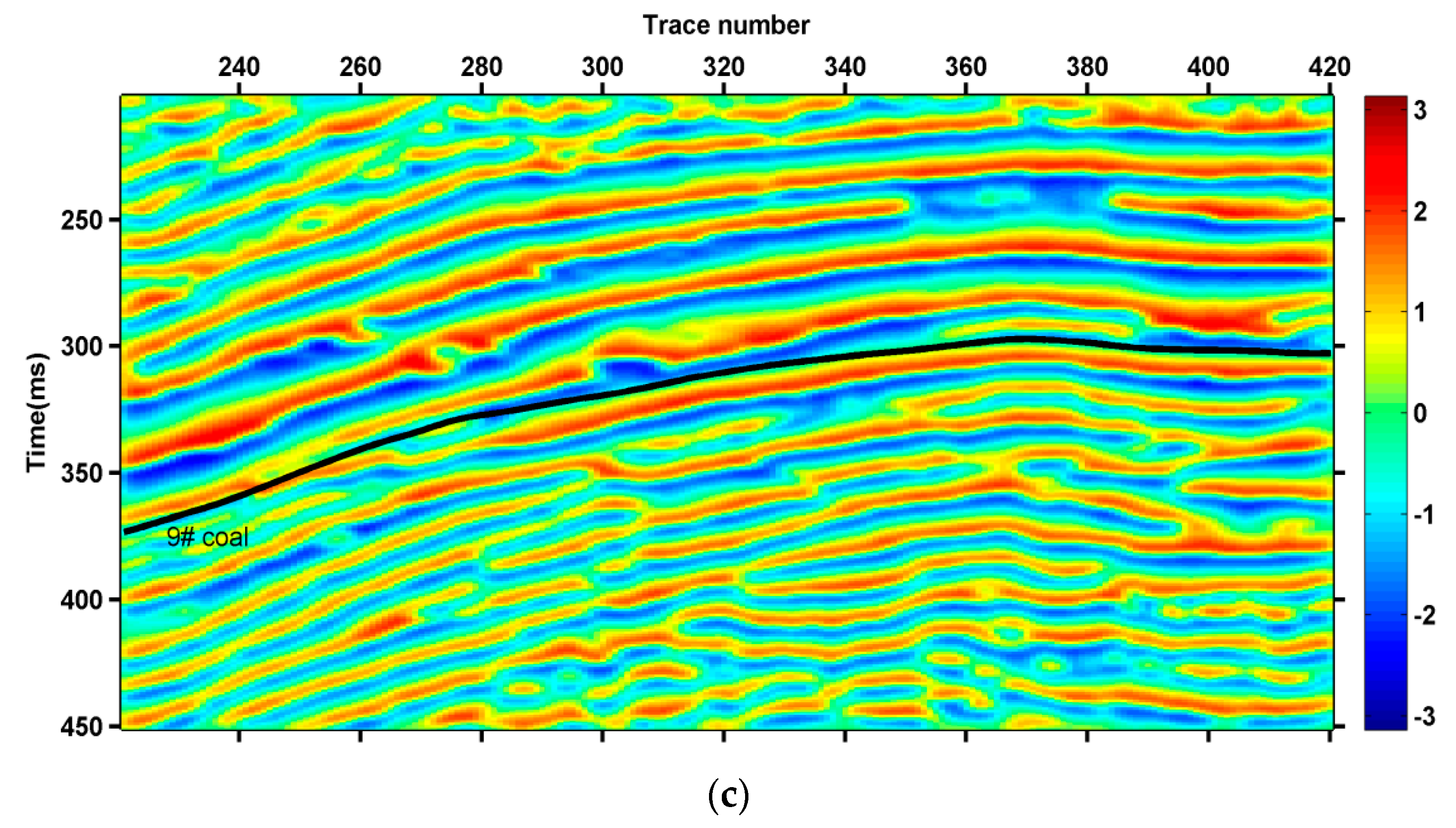
Figure 12, the IMF2 profile based on CEEMD is utilized to extract the instantaneous amplitude, instantaneous frequency and instantaneous phase. As shown in
Figure 12a, the upper 9#coal seam has stronger energy. The instantaneous amplitude shows great lithological differences around 9# coal seam. In
Figure 12b, the lower 9# coal seam has stronger energy, and the instantaneous frequency shows great lithological differences around 9# coal seam. As shown in
Figure 12c, the instantaneous phase clearly shows the continuity and discontinuity of the strata.
Based on drilling data, the top interface of Ordovician limestone exists at about 15 ms below the 9# coal seam. The instantaneous amplitude and instantaneous frequency also show that this area and the 9# coal seam have great lithological differences. At the same time, the instantaneous phase is utilized for preliminary interpretation of the undulations of the top interface. The profile’s Ordovician limestone top interface has better continuity and shows a “left lower and right higher” trend. However, the bifurcation could be found around Trace340. Therefore, it is of great significance to ensure the connectivity between the position and limestone water during later mining to realize coal mine safety.


