A Novel Probabilistic Optimal Power Flow Method to Handle Large Fluctuations of Stochastic Variables

Abstract

The traditional cumulant method (CM) for probabilistic optimal power flow (P-OPF) needs to perform linearization on the Karush–Kuhn–Tucker (KKT) first-order conditions, therefore requiring input variables (wind power or loads) varying within small ranges. To handle large fluctuations resulting from large-scale wind power and loads, a novel P-OPF method is proposed, where the correlations among input variables are also taken into account. Firstly, the inverse Nataf transformation and Cholesky decomposition are used to obtain samples of wind speeds and loads with a given correlation matrix. Then, the K-means algorithm is introduced to group the samples of wind power outputs and loads into a number of clusters, so that in each cluster samples of stochastic variables have small variances. In each cluster, the CM for P-OPF is conducted to obtain the cumulants of system variables. According to these cumulants, the moments of system variables corresponding to each cluster are computed. The moments of system variables for the total samples are obtained by combining the moments for all grouped clusters through the total probability formula. Then, the moments for the total samples are used to calculate the corresponding cumulants. Finally, Cornish–Fisher expansion is introduced to obtain the probability density functions (PDFs) of system variables. IEEE 9-bus and 118-bus test systems are modified to examine the proposed method. Study results show that the proposed method can produce more accurate results than traditional CM for P-OPF and is more efficient than Monte Carlo simulation (MCS).

1. Introduction

Optimal power flow (OPF) has been an important tool for power system operation and planning [1,2]. Traditional OPF problems are based on deterministic models, in which loads, as well as upper and lower bounds of generation, are fixed. Large-scale renewable energies have introduced more uncertainties into power systems [3,4]. Meanwhile, loads fluctuate with large ranges, due to changes of load characteristics and demands. Probabilistic optimal power flow (P-OPF) is a common approach to handle generation and load uncertainties.

References [5,6] provided critical reviews on the probabilistic methods studying the uncertainties in power systems. The methods of solving P-OPF problems could be classified into three categories: simulation methods, approximation methods and analytical methods. Monte Carlo simulation (MCS) [7,8] was used to solve P-OPF problems considering the uncertainties and correlations of input variables. To illustrate the accuracy of MCS, references [9,10] applied the algorithm to a number of benchmark problems and indicated that experimental error could be limited to a very low level through a large number of simulations. Therefore, MCS with a large number of samples is usually utilized as a comparative reference, but it is time-consuming. In order to reduce the computational burden of MCS, some efficient sampling methods such as importance sampling (IS) [11], Latin hypercube sampling (LHS) [12,13] and Latin supercube sampling (LSS) [14] were applied. References [15,16] indicated that quasi-MCS had better performance, based on computational efficiency, than traditional MCS. Correlations among random variables were handled by Cholesky decomposition [12,13,14], copula function [15], pair-copula method [8] and a ninth-order polynomial normal transformation technique (NPNT) [16].

Compared with simulation methods, approximation methods are generally more efficient. Approximation methods consist of point estimate method (PEM) and unscented transformation method (UTM). The 2 m PEM and 2 m + 1 PEM are two widely used point estimate methods. The 2 m PEM was proposed to solve P-OPF in [17,18]. Reference [19] carried out a cost-benefit analysis for a power system with energy storage integration and wind generation using the 2 m PEM. For solving probabilistic load flow (PLF) problems, reference [20] applied the 2 m + 1 PEM to obtain more accurate results than the 2 m PEM. In [21,22], both 2 m and 2 m + 1 PEM were employed to solve P-OPF problems for wind-integration power system. To handle correlations among random variables, Cholesky decomposition was used to modify PEM [22,23,24,25,26,27]. In [25], the modified 2 m + 1 PEM was applicable to P-OPF considering the correlations of wind speeds following different distributions. Another approximation method, UTM, was presented to handle correlations among input variables [5,28]. Approximation methods are powerful to solve P-OPF problems. However, the efficiency decreases as the number of random variables increases, and the accuracy becomes worse for higher order moments of output variables.

Compared with MCS, analytical methods can also reduce computational burden. Reference [29] applied the Gaussian mixture model (GMM) to model non-Gaussian input variables and their correlations. Without denying the advantage in modeling non-Gaussian distributions, the efficiency of GMM decreases as the number of input variables increases. The cumulant method (CM) is one of analytical methods and has the highest computational efficiency. For solving PLF problems, CM and approximation expansions (Gram–Charlier, Edgeworth and Cornish–Fisher expansions) were utilized to obtain cumulants, probability density functions (PDFs) and cumulative distribution functions (CDFs) of output variables [30,31,32]. In addition, correlations among random input variables were taken into account using Cholesky decomposition [33] and joint cumulants [31,34]. In [35], the method of combining CM and GMM was used to model multimodal probability distributions. For solving P-OPF problems, the CM for P-OPF was proposed to obtain the mean values, variance values and PDFs of system variables [36]. In [37], two extensions of the CM for P-OPF were introduced, where limits within the P-OPF problems were handled by combining multiple PDFs to generate final PDFs, and Gram–Schmidt orthogonalization was used to handle correlations of loads.

When the input variables have large fluctuations, the cumulants and PDFs of output variables (voltage magnitude, voltage angle, active power and reactive power of generation units etc.) obtained using the traditional CM could result in significant errors compared with Monte Carlo simulation. The traditional CM for P-OPF first performs the deterministic OPF using the mean values of input variables (such as wind power outputs, loads) to obtain the Karush–Kuhn–Tucker (KKT) first-order conditions, then takes the full derivative of KKT first-order conditions and obtains a linear relationship between input variables and output variables (such as voltage magnitude, voltage angle etc.). Therefore, the linear relationship is obtained at the operating point using the mean values of wind power outputs and loads. When the wind power outputs and loads fluctuate to a value that is far away from the mean value, the operating point has changed. The coefficients of linear relationship obtained at the new operating point could be significantly different from the values obtained at the operating point using the mean values of input variables. The cumulants calculated using the coefficients of linear relationship could have large deviations. Therefore, the PDFs of output variables based on the cumulant method may result in errors. Reference [38] studied the errors resulting from linearization and pointed out that the linear model performed well within small ranges of random variables but would cause large errors when ranges of random variables increased. To tackle this problem, this paper proposes a novel probabilistic optimal power flow method, which can handle large fluctuations and correlations of stochastic variables.

This paper is structured as follows: Section 2 introduces the traditional CM for P-OPF. In Section 3, the theoretical framework of the proposed method is proposed in detail. In Section 4, IEEE 9-bus and 118-bus test systems are used for verifying the proposed method. Finally, conclusions are presented in Section 5.

2. Traditional CM for P-OPF

In the process of the traditional CM for P-OPF, a deterministic OPF model is solved for the mean values of input variables using a Logarithmic Barrier Interior Point Method (LBIPM) [39]. The Hessian is used to formulate the linear relationship between output variables and input variables.

For a power system integrated with wind farms, the deterministic OPF model can be described by the following non-linear optimization problem with equality and inequality constraints [5,25]:

$$\min {{\displaystyle \sum }}_{i=1}^N\left(a_{2i}{P}_{Gi}^2+a_{1i}{P}_{Gi}+a_{0i}\right)$$

(1)

subject to:

$$\begin{gathered} V_i{{\displaystyle \sum }}_{j=1}^N{V}_j\left(G_{ij}\cos {\delta }_{ij}+B_{ij}\sin {\delta }_{ij}\right)+P_{Di}-P_{Gi}-P_{Wi}=0 \\ {V}_i{{\displaystyle \sum }}_{j=1}^N{V}_j\left(G_{ij}\sin {\delta }_{ij}-B_{ij}\cos {\delta }_{ij}\right)+Q_{Di}-Q_{Gi}-Q_{Ci}=0 \\ {P}_{Gi}^{\min }\le P_{Gi}\le P_{Gi}^{\max } \\ {Q}_{Gi}^{\min }\le Q_{Gi}\le Q_{Gi}^{\max } \\ {V}_i^{\min }\le V_i\le V_i^{\max } \\ \left|T_l\right|\le T_l^{\max } \\ \left(i=1,\cdots ,N; l=1,\cdots ,NT\right) \end{gathered}$$

(2)

where $P_{Gi}$ and $Q_{Gi}$ are the active and reactive power generation of conventional generator at bus $i$. $a_{2i}$, $a_{1i}$ and $a_{0i}$ are cost coefficients of the generator at bus $i$. $P_{Wi}$ is the active power output of the wind farm at bus $i$. $Q_{Ci}$ is the reactive power injected by the compensation device at bus $i$. $P_{Di}$ and $Q_{Di}$ are the active and reactive loads at bus $i$. $V_i$ is the magnitude of voltage at bus $i$. ${\delta }_{i_j}$ is the phase angle difference between bus $i$ and $j.$ $G_{ij}$ and $B_{ij}$ are the real and imaginary parts of the element in the bus admittance matrix, respectively. $T_l$ is the complex power flow of branch $l$. N is the number of buses, and $NT$ is the number of branches. $P_{Gi}^{\min }$, $P_{Gi}^{\max }$, $Q_{Gi}^{\min }$, $Q_{Gi}^{\max }$, $V_i^{\min }$ and $V_i^{\max }$ are the lower and upper bounds of corresponding variables. $T_l^{\max }$ is the line rating of branch $l$.

In the P-OPF studies, wind power output and load at each bus should be treated as random input variables. The wind power output is calculated using the following equation:

$$P_{Wi}=\{\begin{array}{cc}0& ( 0<S{W}_i<V_{ci})\hfill \\ \left(A_1+B_1\times S{W}_i+C_1\times S{W}_i\right)\times P_r& ( V_{ci}\le S{W}_i<V_r)\hfill \\ P_r & (V_r\le S{W}_i<V_{co})\hfill \\ 0& \left(S{W}_i\ge V_{co}\right)\hfill \end{array}$$

(3)

where $S{W}_i$ is the wind speed of the wind farm at bus $i$, and $P_r$ is the rated power of the wind farm. $V_{ci}$, $V_r$ and $V_{co}$ are the cut-in, rated and cut-out speeds of the wind farm, respectively. $A_1$, $B_1$ and $C_1$ are coefficients [40]. The wind power output can be modeled as a negative load, and its power factor is kept constant [5].

References [36,37] built the model of CM for P-OPF with the load at each bus as a random input variable. In this paper, wind power output is also treated as a random input variable and incorporated into the computational model. The procedure of CM for P-OPF is summarized as follows:

• Take the mean values of wind power outputs and loads, and solve the aforementioned deterministic OPF model using LBIPM.
• Obtain the KKT first-order conditions, when the optimization is converged:

  $$F\left(Y\right)=0$$

  (4)

  where $F$ is the set of equations defining the KKT first-order conditions. $Y$ is a vector consisting of magnitude and angle of voltage at each bus, active and reactive generation of each conventional generator, slack variables and Lagrange multipliers.
• Treat loads and wind power outputs as random input variables, and formulate new KKT first-order conditions:

  $$F\left(Y,L,W\right)=0$$

  (5)

  where $L$ and $W$ are the vectors of load and wind power output at each bus, respectively.
• Take the full derivative of (5), and find a linear relationship between input variables and output variables:

  $$H\Delta Y+H_L\Delta L+H_W\Delta W=0$$

  (6)

  where $H$ is the Hessian of the Lagrangian function with respect to $Y$ when the optimization is completed. $\Delta Y$, $\Delta L$ and $\Delta W$ are vectors of the changes in $Y$, $L$ and $W$. $H_L$ and $H_W$ are obtained by taking the partial derivatives of (5) with respect to $L$ and $W$, respectively. Equation (6) can be reformed as the following equation:

  $$\begin{array}{ccc}\Delta Y& =& -H^{-1}{H}_L\Delta L-H^{-1}{H}_W\Delta W\hfill \\ & =& H_1\Delta L+H_2\Delta W\hfill \end{array}$$

  (7)

  where $H^{-1}$ is the inverse of the obtained Hessian, $H_1=-H^{-1}{H}_L$, and $H_2=-H^{-1}{H}_W$.
  From Equation (7), an unknown variable $y_i$ can be formulated as a linear combination of known input variables (loads and wind power outputs):

  $$\begin{array}{ccc}{y}_i& =& y_{i0}+\Delta y_i\hfill \\ & =& y_{i0}+{\displaystyle {\displaystyle \sum }_{j=1}^{NL}}{h}_{1ij}(l_j-l_{j0})+{\displaystyle {\displaystyle \sum }_{j=1}^{NW}}{h}_{2ij}(w_j-w_{j0})\hfill \\ & =& y{s}_{i0}+{\displaystyle {\displaystyle \sum }_{j=1}^{NL}}{h}_{1ij}{l}_j+{\displaystyle {\displaystyle \sum }_{j=1}^{NW}}{h}_{2ij}{w}_j\hfill \end{array}$$

  (8)

  where $y_{i0}$ is the value of $y_i$ evaluated by the deterministic OPF in step 1. $\Delta y_i$ is the change of $y_i$. $h_{1ij}$ and $h_{2ij}$ are the values at the i-th row and j-th column of $H_1$ and $H_2$, respectively. $l_j$ and $w_j$ are the j-th variables in $L$ and $W$, respectively. $l_{j0}$ and $w_{j0}$ are the mean values of $l_j$ and $w_j$, respectively. $NL$ is the number of load variables, and $NW$ is the number of wind power variables. $y{s}_{i0}=y_{i0}-{{\displaystyle \sum }}_{j=1}^{NL}{h}_{1ij}{l}_{j0}-{{\displaystyle \sum }}_{j=1}^{NW}{h}_{2ij}{w}_{j0}$.
• If the known input variables (loads and wind power outputs) are independent of each other, the cumulants of unknown output variables can be computed by a linear combination of cumulants of known input variables based on the property of cumulants (see Appendix A):

  $${\gamma }_v^{y_i}=\{\begin{array}{ll}{\displaystyle {\displaystyle \sum }_{j=1}^{NL}}{h}_{1ij}{\gamma }_1^{l_j}+{\displaystyle {\displaystyle \sum }_{j=1}^{NW}}{h}_{2ij}{\gamma }_1^{w_j}+ y{s}_{i0}\hfill & \left(v=1\right)\hfill \\ {\displaystyle {\displaystyle \sum }_{j=1}^{NL}}{h}_{1ij}^v{\gamma }_v^{l_j}+{\displaystyle {\displaystyle \sum }_{j=1}^{NW}}{h}_{2ij}^v{\gamma }_v^{w_j}\hfill & (v>1)\hfill \end{array}$$

  (9)

  where ${\gamma }_v^{y_i}$ is the v-th order cumulant of $y_i$. ${\gamma }_v^{l_j}$ and ${\gamma }_v^{w_j}$ are the v-th order cumulants of $l_j$ and $w_j$, respectively.

3. The Proposed Method for P-OPF

The traditional CM for P-OPF requires that input variables have small variances. In [36,37], loads were modeled as normal distributions with a variance of 99% confidence interval equal to ±10% of mean values. It is not reasonable if the wind power is assumed as a normal distribution with a variance of 99% confidence interval equal to ±10% of the mean value because wind power can vary between 0 MW and its rated power. Based on our studies, the traditional CM for P-OPF will have significant errors if the load’s standard deviation is larger than 5% of its mean and the ratio of the total rated wind power to the total system load exceeds 10%. Therefore, a power system has large fluctuations when the load’s standard deviation is larger than 5% of its mean and the ratio of the total rated wind power to the total system load exceeds 10%. To solve P-OPF problems for power systems with large fluctuations of stochastic variables, the proposed method treats samples of input variables (loads and wind power outputs) as points in a multi-dimensional space and groups them into a number of clusters using K-means algorithm. The points in the same cluster are close to one another, so in each cluster samples of input variables have small variances. The total probability formula is used to combine moments obtained using CM for P-OPF in each cluster to compute the final moments of output variables. Section 3.1 introduces the overall procedure of the proposed method, which contains seven steps. Section 3.2, Section 3.3, Section 3.4, Section 3.5 and Section 3.6 introduce key steps in detail.

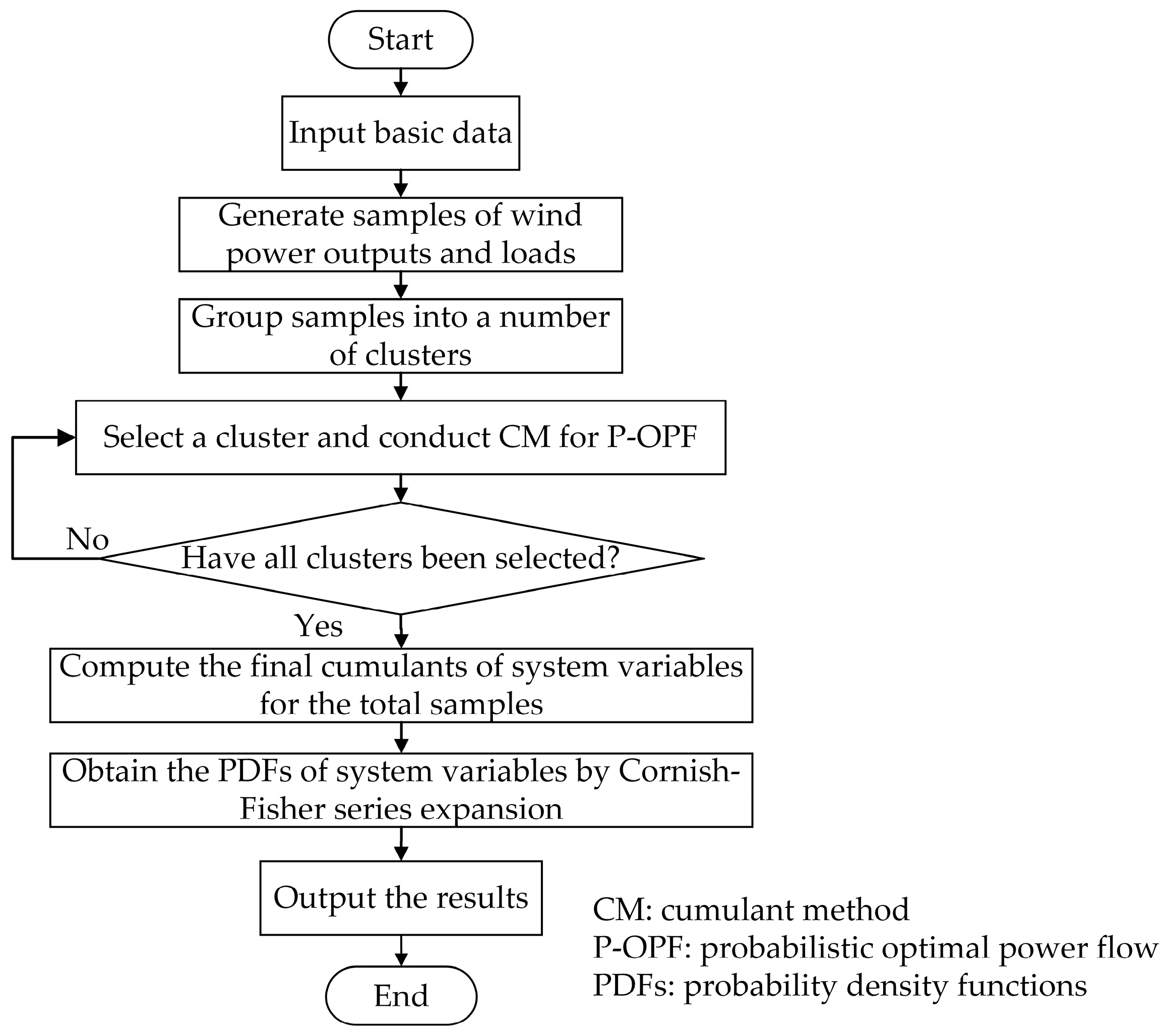
3.1. The Overall Procedure of the Proposed Method

The flowchart of the proposed method in this paper is presented in Figure 1. The overall procedure of the proposed method can be summarized as follows:

• Input the basic data, including network data, the distribution functions of wind speeds and loads, and the correlation matrix.
• Generate samples of correlated wind speeds and loads using the method introduced in [25,41]. Then, calculate wind power outputs according to Equation (3).
• Group the samples of wind power outputs and loads into a number of clusters using the K-means algorithm.
• In each cluster, the CM for P-OPF considering correlations among input variables is applied. Firstly, the samples for each cluster are converted to uncorrelated samples. Then, the cumulants of uncorrelated input variables are calculated based on uncorrelated samples [33]. Finally, the CM for P-OPF is applied to compute the cumulants of system variables for each cluster.
• Compute the final cumulants of system variables for the total samples.
• PDFs of system variables are produced by Cornish–Fisher series expansion [42].
• Output the cumulants and PDFs of system variables.

3.2. Generating Samples of Correlated Wind Power Outputs and Loads

For P-OPF problems, it is usually assumed that loads follow normal distribution functions and wind speeds follow Weibull distribution functions. In the process of the proposed method, based on the known distribution functions, samples of wind speeds and loads, which meet the given correlation matrix, are first generated by the method introduced in [25,41]. Then, the wind power outputs are calculated by (3).

3.3. Application of the K-Means Algorithm to Group Samples into Clusters

The samples of wind power outputs and loads can be expressed as $X=\left[X_1,X_2,\cdots ,X_i,\cdots ,X_n\right]$, where $X_i$ is a column vector of a sample for a specific input variable (wind power or load). The samples of input variables (loads and wind power outputs) are treated as points in a multi-dimensional space as shown in Figure 2.

In order to obtain the samples with smaller variances, the clustering algorithm is intended to be used to group all the samples into a number of clusters. Hierarchical clustering and K-means algorithm are two common approaches for clustering. However, the hierarchical clustering algorithm can only be used for relatively small datasets [43]. Therefore, K-means algorithm is applied in this paper. The K-means algorithm procedure is as follows:

(1).

Pick initial mean values of all clusters, which are defined as the following equations:

$$M_0=\left[\begin{array}{c}{m}_1\\ m_2\\ ⋮\\ m_j\\ ⋮\\ m_k\end{array}\right]$$

(10)

$$m_j=\left[x_{1j}^0,x_{2j}^0,\cdots ,x_{ij}^0,\cdots ,x_{nj}^0\right]$$

(11)

where $M_0$ is a multi-dimensional vector comprised of initial mean values of all clusters, $k$ is the pre-set number of clusters, $m_j$ is the mean value vector of cluster $j$, and $x_{ij}^0$ is the picked initial mean value of the variable $i$ in cluster $j$.

(2).

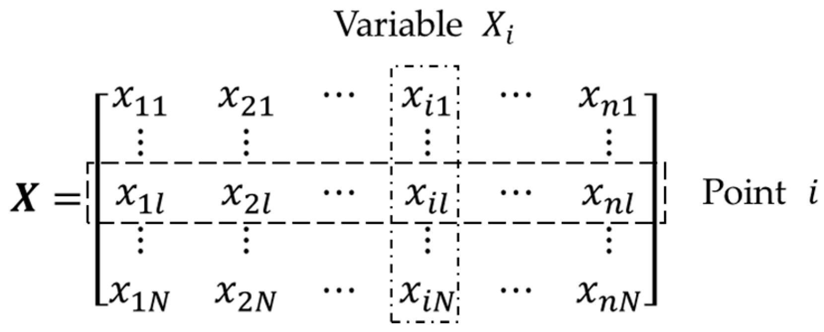
Calculate Euclidean distances from each point to each cluster mean according to the following equation:

$$d\left(l,j\right)=\sqrt{{\left(x_{1l}-x_{1j}^0\right)}^2+{\left(x_{2l}-x_{2j}^0\right)}^2+\cdots +{\left(x_{il}-x_{ij}^0\right)}^2+\cdots +{\left(x_{nl}-x_{nj}^0\right)}^2}$$

(12)

where $d\left(l,j\right)$ is the Euclidean distance from point $l$ to the mean of clusters $j$, point $l$ is expressed as $\left[x_{1l}, x_{2l}, \cdots , x_{il}, \cdots , x_{nl}\right]$, and $x_{il}$ is the l-th element of $X_i$.

(3).

Assign every point to the nearest cluster according to the Euclidean distances, and update the mean values of all clusters.

(4).

Repeat steps 2 and 3 until points in each cluster are no longer changed.

In this process, the performance of the K-means algorithm is affected by initial values of $M_0$. It is desirable that the $k$ initial points in $M_0$ are as far away from each other as possible. Therefore, in this paper, preliminary clustering is performed using a random 10% sample of $X$. The final mean values of preliminary clustering are used as initial mean values of the K-means algorithm.

In each cluster, each point is close to one another, so that there is a small variance for a variable sample. This property ensures that, in each cluster, the CM for P-OPF can be applied to solving P-OPF problems within acceptable errors.

3.4. The Method of Handling Correlations among Input Variables

CM requires that input variables are independent. In this paper, the Cholesky decomposition algorithm [33,44] is applied to convert correlated variables to independent variables. This algorithm is a reasonable solution for a normal distribution vector with a mean of zero [45]. However, there exist errors for a non-normal distribution vector.

Before applying the Cholesky decomposition algorithm, this paper proposes performing standardization for a multi-dimensional and non-normal distribution vector $W$ (wind power variables) first using Equation (13):

$$w_i^{\prime }=\frac{w_i-E_{w_i}}{{\delta }_{w_i}}$$

(13)

where $w_i$ is a variable in $W$, $E_{w_i}$ and ${\delta }_{w_i}$ are respectively mean and standard deviation of $w_i$, and $w_i^{\prime }$ is the standardized variable corresponding to $w_i$.

The correlation matrix of $W^{\prime }$ is usually a positive definite matrix, which can be decomposed by the Cholesky decomposition algorithm as the following equation:

$$C_{W^{\prime }}=G^{\prime }{G^{\prime }}^T$$

(14)

where $C_{W^{\prime }}$ is the correlation matrix of $W^{\prime }$ and can be calculated according to the samples of $W^{\prime }$, and $G^{\prime }$ is a lower triangular matrix.

The standardized vector $W^{\prime }$ can be transformed to a linear combination of an uncorrelated vector $U$ by (15):

$$W^{\prime }=G^{\prime }U$$

(15)

Assume that a diagonal matrix D is defined as:

$$D=\mathrm{diag}\left({\delta }_{w_1}{\delta }_{w_2}\cdots {\delta }_{w_{NW}}\right)$$

(16)

where $NW$ is the number of wind power variables.

Based on Equations (13), (15) and (16), the linear relationship between $W$ and $U$ can be formulated as follows:

$$\begin{array}{ccc}W& =& D{W}^{\prime }+{\left[E_{w_1}, E_{w_2}, \cdots , E_{w_l} \right]}^{\mathrm{T}}\hfill \\ & =& NU+E\hfill \end{array}$$

(17)

where $N=D{G}^{\prime }$ and $E={\left[E_{w_1},E_{w_2},\cdots ,E_{w_l}\right]}^{\mathrm{T}}$.

It can be seen from Equation (17) that dependent input variables can be converted to a linear combination of uncorrelated variables, which can be easily incorporated into Equation (8) to formulate a new linear combination. This method can also be applied to handling the correlations between loads and wind power outputs.

3.5. Computation of the Cumulants of System Variables

According to the algorithms introduced in the above subsections, the cumulants of system variables in each cluster can be obtained. The next step is to calculate the final cumulants of system variables for the total samples. This paper adopts a new method of computing the moments of system variables for the total samples by combining the moments of system variables for all clusters, after the moments of system variables corresponding to each cluster are calculated.

The procedure of computing the final cumulants of system variables for the total samples can be summarized as follows:

(1).

In each cluster, cumulants of a system variable for each cluster can be obtained based on the algorithms introduced in Section 3.2, Section 3.3 and Section 3.4. The moments of the system variable for each cluster are computed using the following equation:

$${\alpha }_v^i=\{\begin{array}{ll}{\gamma }_1^i\hfill & \left(v=1\right)\hfill \\ {\gamma }_v^i+{\displaystyle {\displaystyle \sum }_{j=1}^{v-1}}{C}_{v-1}^j{\alpha }_j^i{\gamma }_{v-j}^i\hfill & (v>1)\hfill \end{array}$$

(18)

where ${\alpha }_v^i$ is the v-th order moment of a variable for cluster $i$, ${\gamma }_v^i$ is the v-th order cumulant of a variable for cluster $i$, and $C_{v-1}^j$ is a combination of $j$ elements from v − 1 different elements.

(2).

The property that moments meet the total probability formula is applied to combine the moments of the system variable for all clusters. The moments of the system variable for the total samples are calculated using the following equation:

$${\alpha }_v={\displaystyle \sum }_{i=1}^k{p}_i\times {\alpha }_v^i$$

(19)

where ${\alpha }_v$ is the v-th order moment of a system variable for the total samples, k is the number of clusters, and $p_i$ is the proportion of the number of elements in cluster $i$ to the total samples.

(3).

The final cumulants of the system variable for the total samples are obtained using the following equation:

$${\gamma }_v=\{\begin{array}{ll}{\alpha }_1\hfill & \left(v=1\right)\hfill \\ {\alpha }_v-{\displaystyle {\displaystyle \sum }_{j=1}^{v-1}}{C}_{v-1}^j{\alpha }_j{\gamma }_{v-j}\hfill & (v>1)\hfill \end{array}$$

(20)

where ${\gamma }_v$ is the v-th order cumulant of a system variable for the total samples.

3.6. Computation of PDFs of System Variables

Compared with Gram–Charlier A series expansion and Edgeworth series expansion, Cornish–Fisher series expansion works better for non-Gaussian distribution variables [42]. This paper adopts Cornish–Fisher series expansion to obtain PDFs of system variables. This method is introduced in detail in [42].

4. Case Studies

IEEE 9-bus and 118-bus test systems [46] are modified to verify the accuracy and efficiency of the proposed method. Two wind farms are added into the IEEE 9-bus test system, and three wind farms are added into the IEEE 118-bus test system. The rated capacities of wind farms and corresponding buses are listed in

Table 1. The rated capacities of wind farms and corresponding buses.

Systems	Buses Connected with Wind Farms	Rated Capacities (MW)
IEEE 9-Bus Test System	1, 3	60
IEEE 118-Bus Test System	59, 80, 90	250

. It is assumed that the cut-in, rated and cut-out speeds are 3 m/s, 13 m/s and 25 m/s, respectively. The wind farm power factor is assumed as 0.85 lag [47].

The parameters of the objective functions are taken from MATPOWER files [46]. In each case, Monte Carlo Simulations (MCS) are performed with 40,000 samples, whose results are treated as reference for other methods. The traditional CM without consideration of correlations of input variables (UCCM) and with consideration of correlations of input variables (CCCM) using the method introduced in [37] are also performed to demonstrate the accuracy of the proposed method. The absolute percent error (APE) of mean and standard deviation values are calculated to measure the errors.

All the cases are tested using a personal computer with a dual-core 2.6-GHz processor and 8-GB of RAM.

4.1. The Modified IEEE 9-Bus Test System

For the IEEE 9-bus test system, the total system load is modeled as a normal distribution with the mean value equal to the nominal value and the standard deviation equal to 10% of the mean value. The load at each bus varies with the total system load according to its original percentage of the total load, and its power factor is kept constant. Wind speeds are modeled as Weibull distributions, whose parameters are presented in

Table 2. Parameters of Weibull distributions (modified IEEE 9-bus test system).

Wind Speed Distribution	Shape Parameter	Scale Parameter
W1 (Connected to Bus 1)	1.732	6.611
W2 (Connected to Bus 3)	2.036	7.933

[48]. The correlation coefficient of wind speeds is 0.76.

4.1.1. Application of the K-Means Algorithm to Group Samples into Clusters

The samples of wind power outputs and the total system load have been generated using the method introduced in Section 3.2. The mean values of these samples are 10.5880 MW, 15.0741 MW and 315.1020 MW, respectively. The standard deviation values of these samples are 16.1379 MW, 18.4307 MW and 31.4904 MW, respectively. The K-means algorithm is applied to group these samples into 25 clusters. In order to measure the fluctuations of input variables for all clusters, the mean, maximum and minimum values of standard deviation values of input variables for all clusters are calculated, as shown in

Table 3. Statistics of standard deviation values for all clusters.

Input Variable	${\mathit{\delta }}_{\mathit{m}\mathit{e}\mathit{a}\mathit{n}} \left(\mathbf{MW}\right)$	${\mathit{\delta }}_{\mathit{m}\mathit{a}\mathit{x}}$ $\left(\mathbf{MW}\right)$	${\mathit{\delta }}_{\mathit{m}\mathit{i}\mathit{n}}$ $\left(\mathbf{MW}\right)$
Wind Power 1 (Connected to Bus 1)	7.0850	10.9982	2.8596
Wind Power 2 (Connected to Bus 3)	7.2758	11.6619	3.6242
Total System Load	8.1510	14.3702	3.4837

. It can be seen from Table 3 that input variables for each cluster have much smaller standard deviation values than those for the total samples, which indicates that input variables for each cluster have smaller fluctuations.

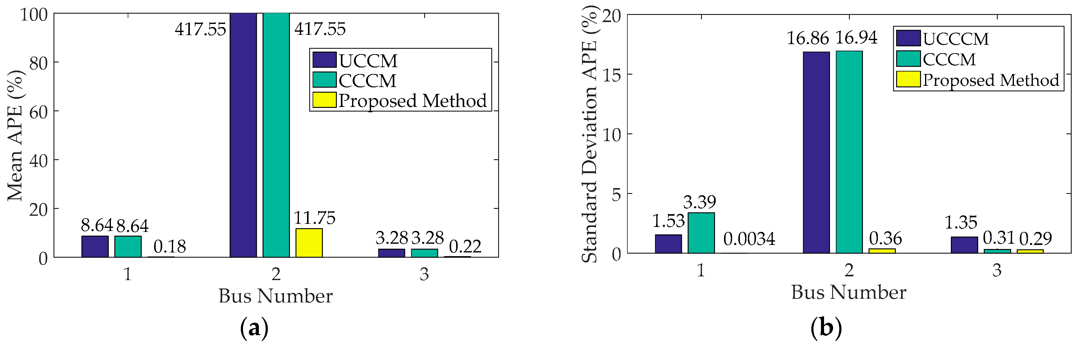
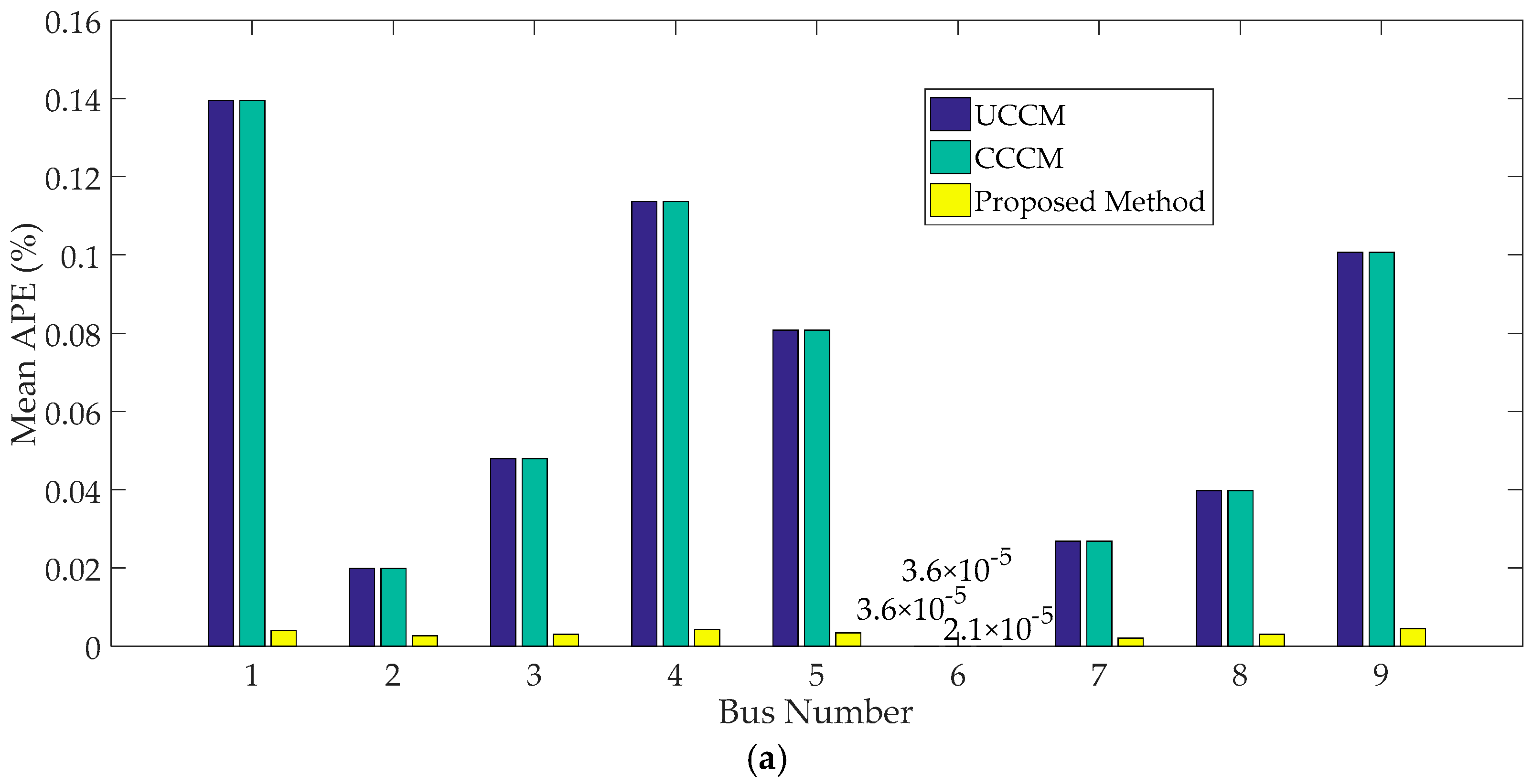
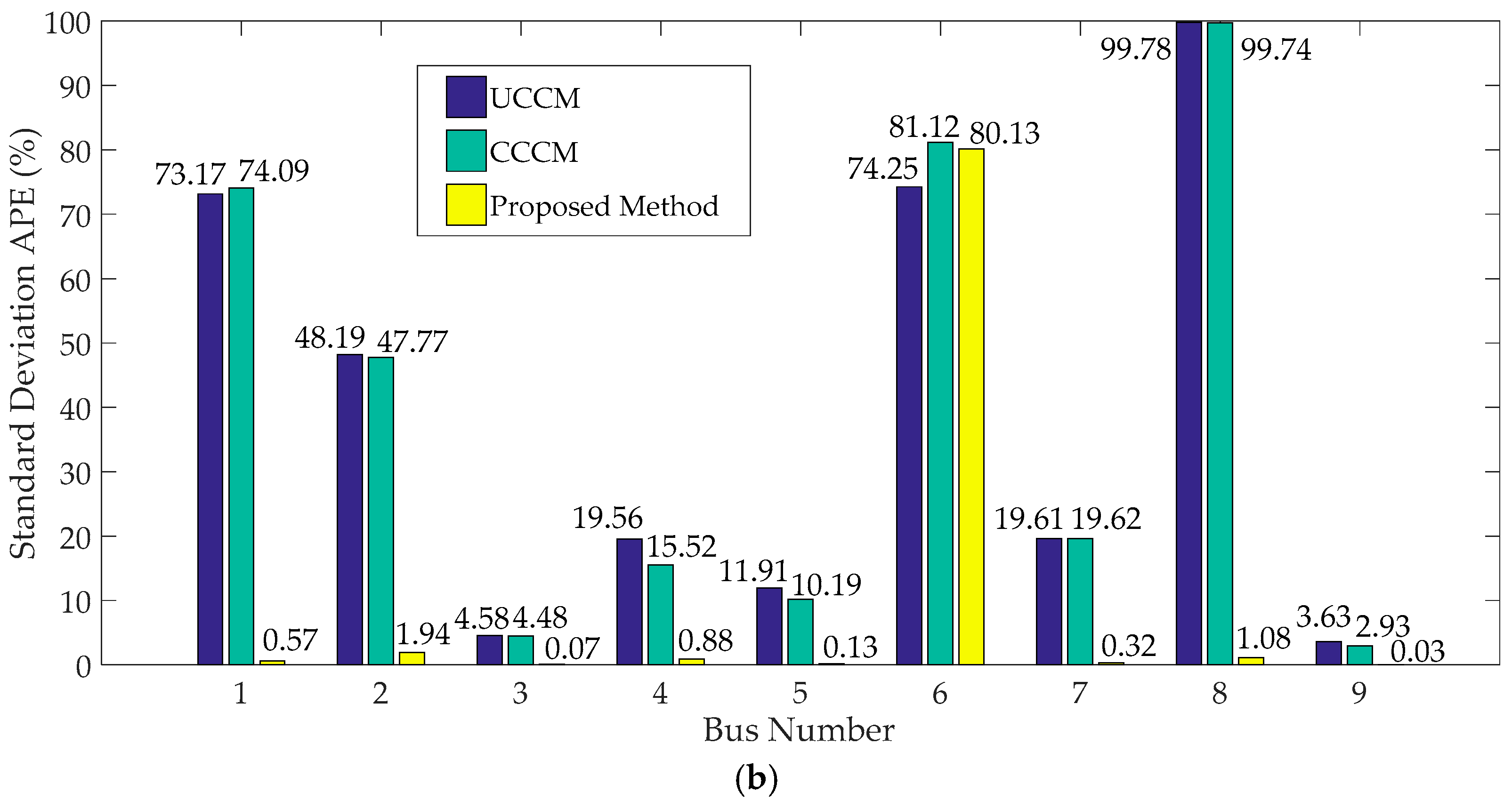
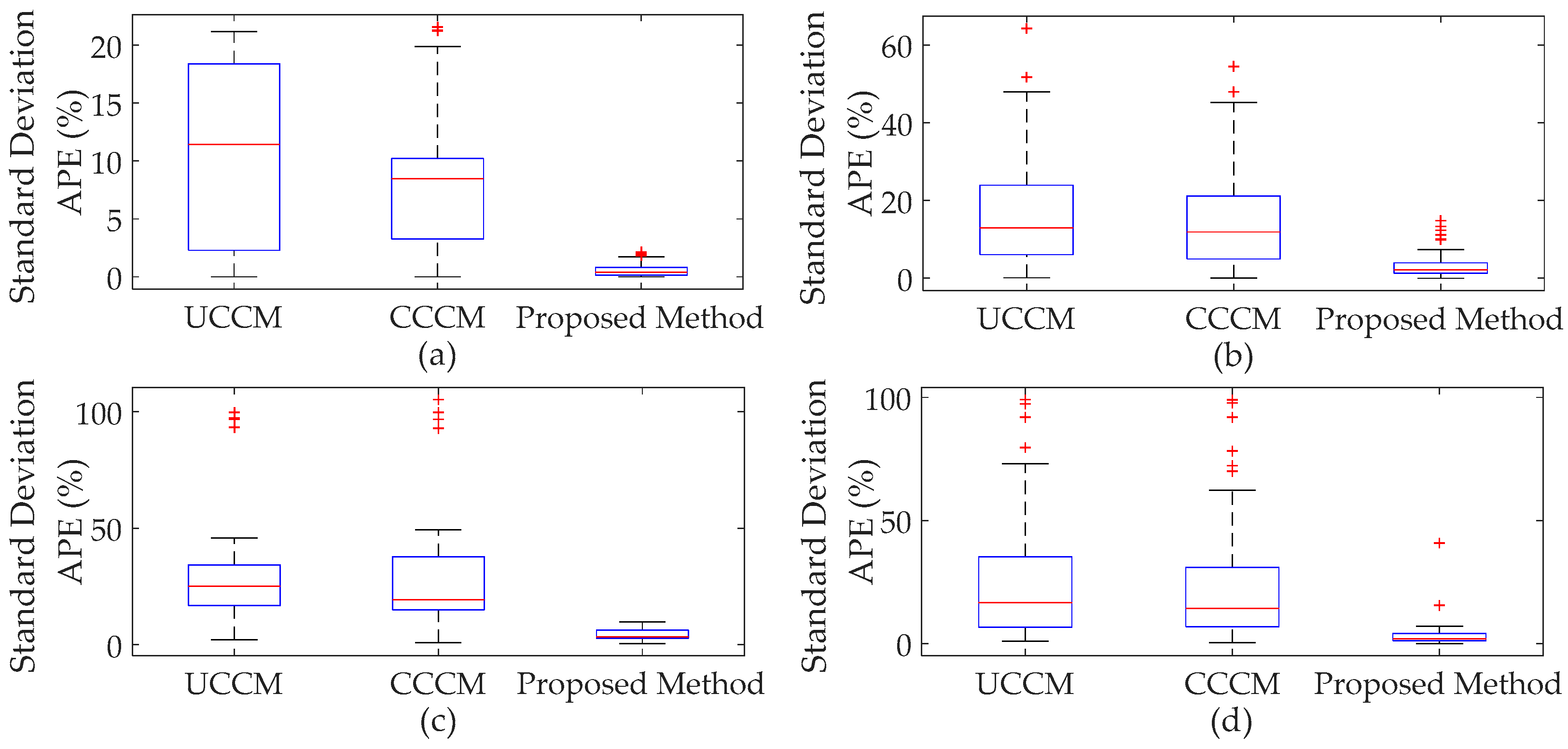
4.1.2. Cumulants of System Variables and Comparison

In each cluster, the CM for P-OPF considering the correlation of wind power outputs is conducted to obtain the cumulants of system variables. These obtained cumulants are used to calculate the final cumulants for the total samples using the method introduced in Section 3.5.

The mean (the first order cumulant) and the standard deviation (the square root of the second order cumulant) are calculated as the most important results of P-OPF. The standard deviation provides an indicator for the fluctuation of each system variable.

Table 4. Comparison of generation cost (modified IEEE 9-bus test system).

Algorithm	Mean	Mean APE	Standard Deviation	Standard Deviation APE
MCS	4769.75	\	992.97	\
UCCM	4697.13	1.52%	910.72	8.28%
CCCM	4697.13	1.52%	1022.13	2.94%
Proposed Method	4765.08	0.10%	994.90	0.19%

shows the results of generation cost obtained using different methods. It can be seen that all absolute percent error (APE) values obtained using the proposed method are much smaller than those obtained using UCCM and CCCM.

Figure 3 illustrates the results of generators’ reactive power, and Figure 4 illustrates the results of voltage magnitude at each bus. In Figure 3, it can be seen that the proposed method has much better performance, based on mean and standard deviation APE. It is noteworthy that the mean APE value of reactive power generation at bus 2 obtained using the proposed method is relatively large at 11.75%. The actual error is only −0.0137 MVar. In Figure 4, it is obvious that most standard deviation APE values obtained using the proposed method are extremely small and much smaller than those obtained using UCCM and CCCM. It should be pointed out that the standard deviation APE value of voltage magnitude at bus 6 using the proposed method is 80.13%. However, the standard deviation of voltage magnitude at bus 6 obtained using MCS is only 7.20 × 10⁻⁶ p.u., and the actual error is 5.77 × 10⁻⁶ p.u. Moreover, the ratio of its standard deviation to mean, namely coefficient of variation (CV), is only 0.0007%, which is much smaller than those of other variables. The CV is a standardized measure of dispersion of a probability distribution, so that the quite small value indicates that this variable is almost deterministic, compared with others. Therefore, this kind of variables, whose CV values are very small, can be treated as constants and not analyzed as probabilistic variables.

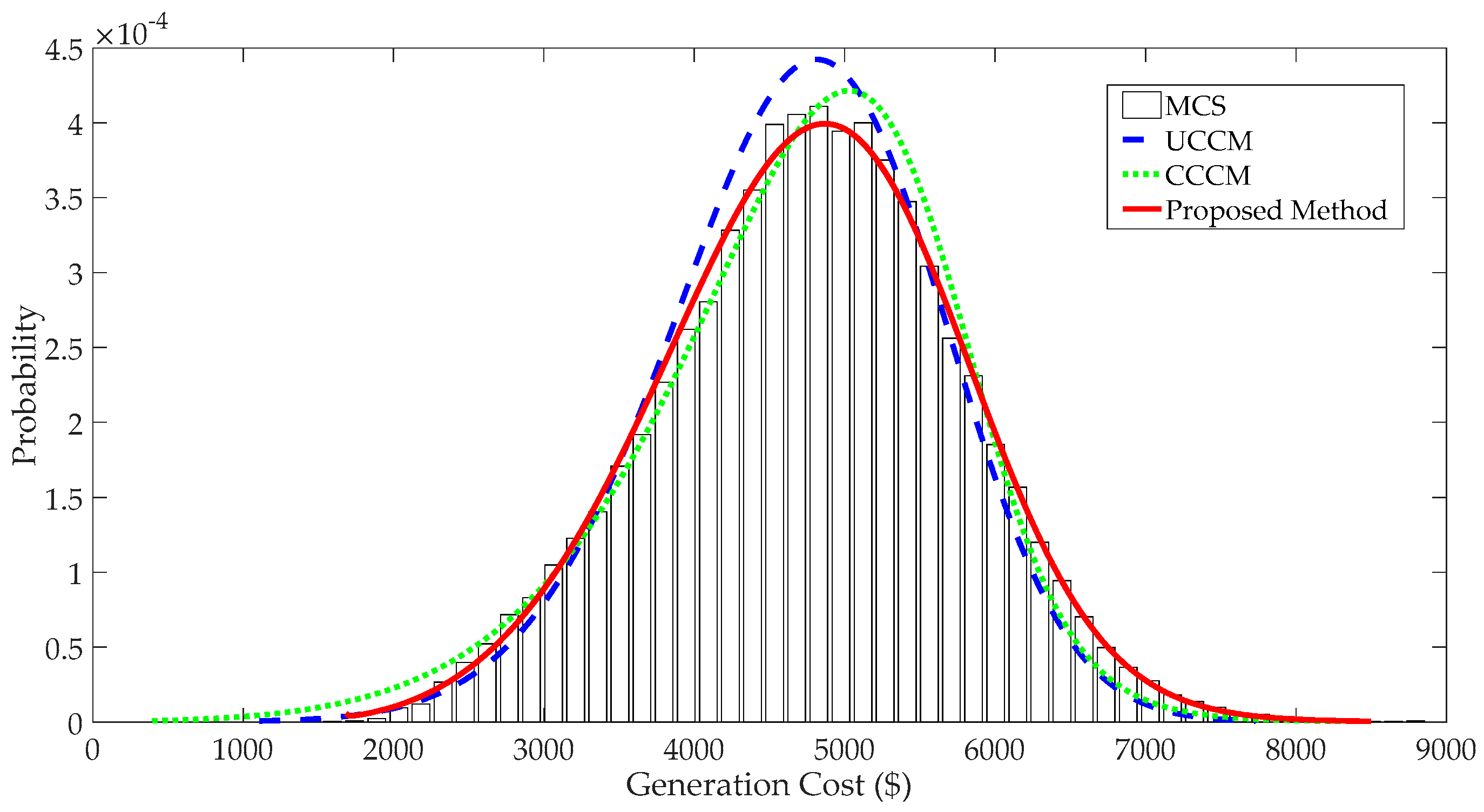
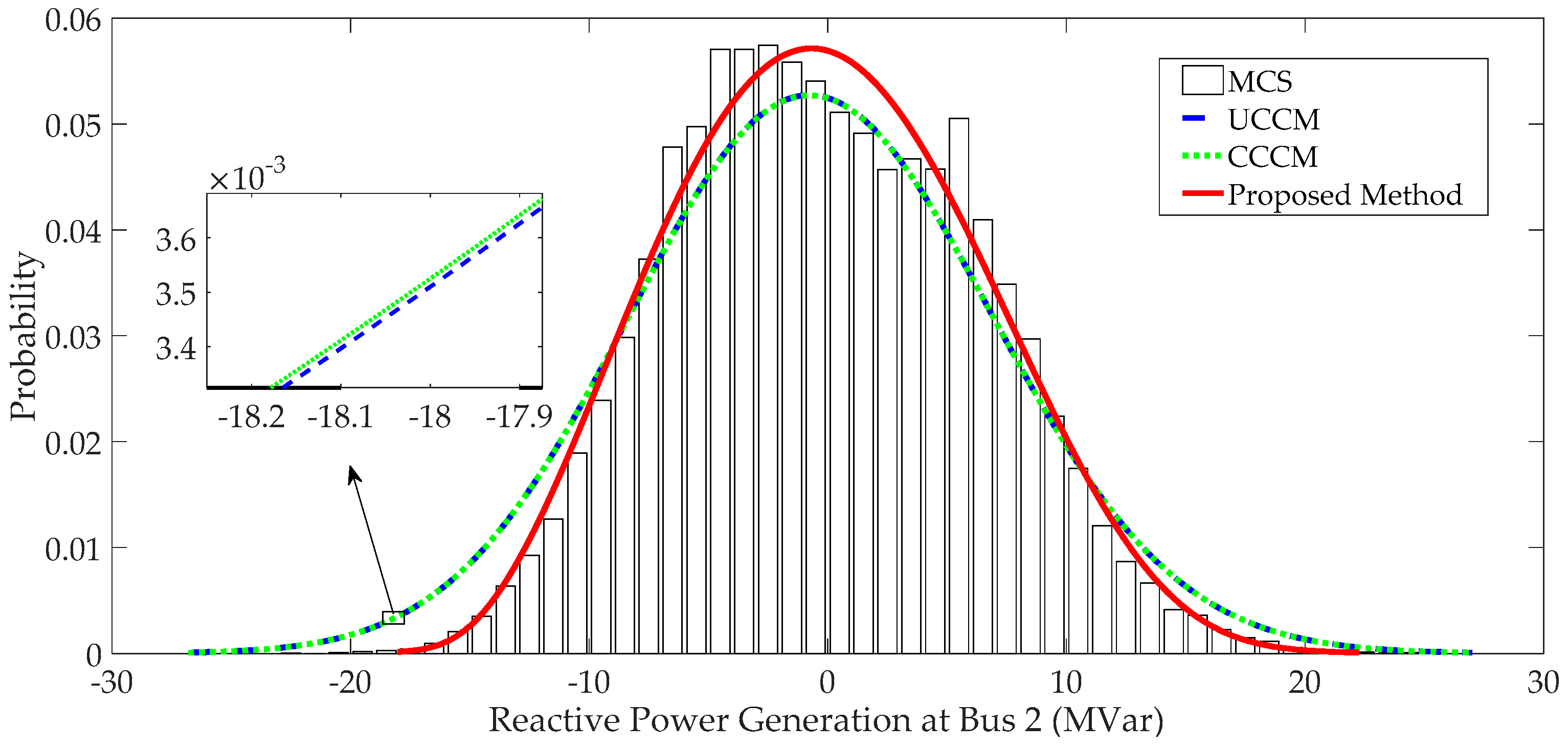
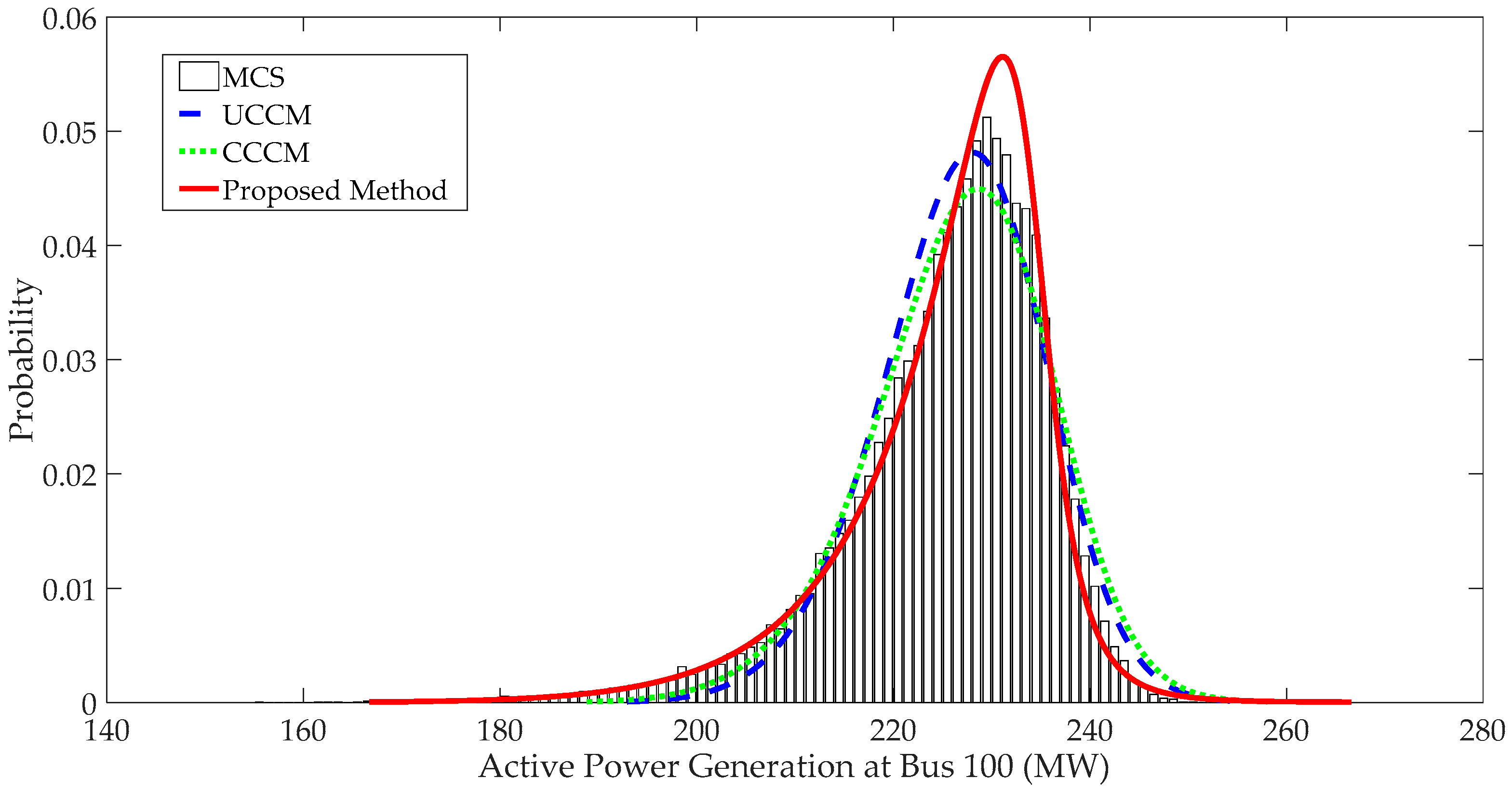
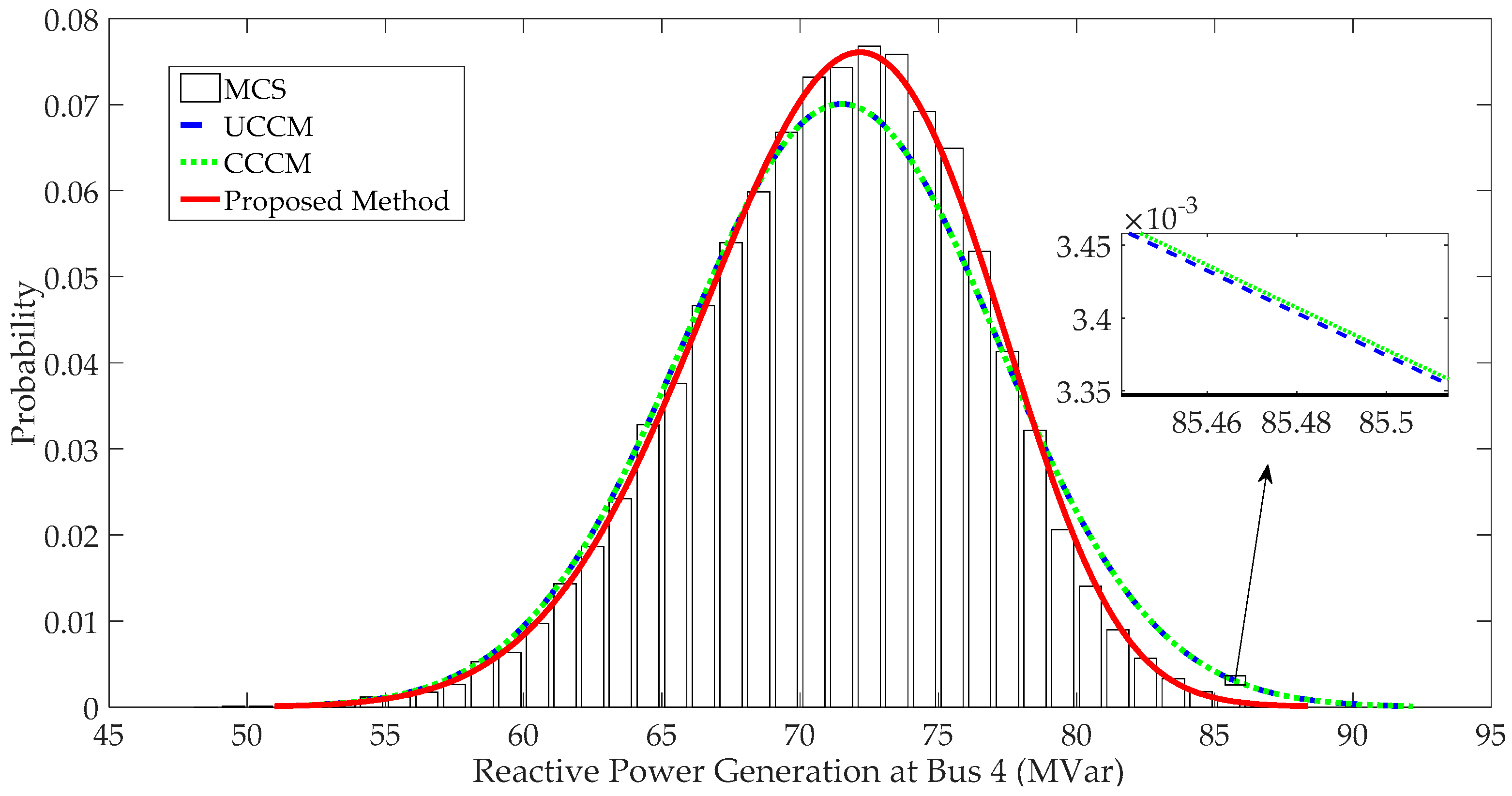
4.1.3. PDFs of System Variables and Comparison

Cornish–Fisher series expansion is applied to produce the PDFs of output variables. The PDFs of generation cost and reactive power generation at bus 2 are shown in Figure 5 and Figure 6. It can be observed that the curves obtained using the proposed method match the histograms obtained using MCS better than those obtained using UCCM and CCCM. Especially, curves obtained using UCCM and CCCM have significant errors at the tails of curves, which also demonstrates the shortcoming of traditional CM for P-OPF as discussed in Section 1. Moreover, the computation time of the proposed method is hundreds of times less than that using MCS as listed in

Table 5. Computation time table for the modified IEEE 9-bus test system.

Algorithm	Time (s)
MCS	1912.72
UCCM	4.21
CCCM	4.58
Proposed Method	6.27

. In summary, the traditional CM has significant errors when solving P-OPF problems with large fluctuations of stochastic variables. On the contrary, the proposed method performs well, based on the accuracy and efficiency.

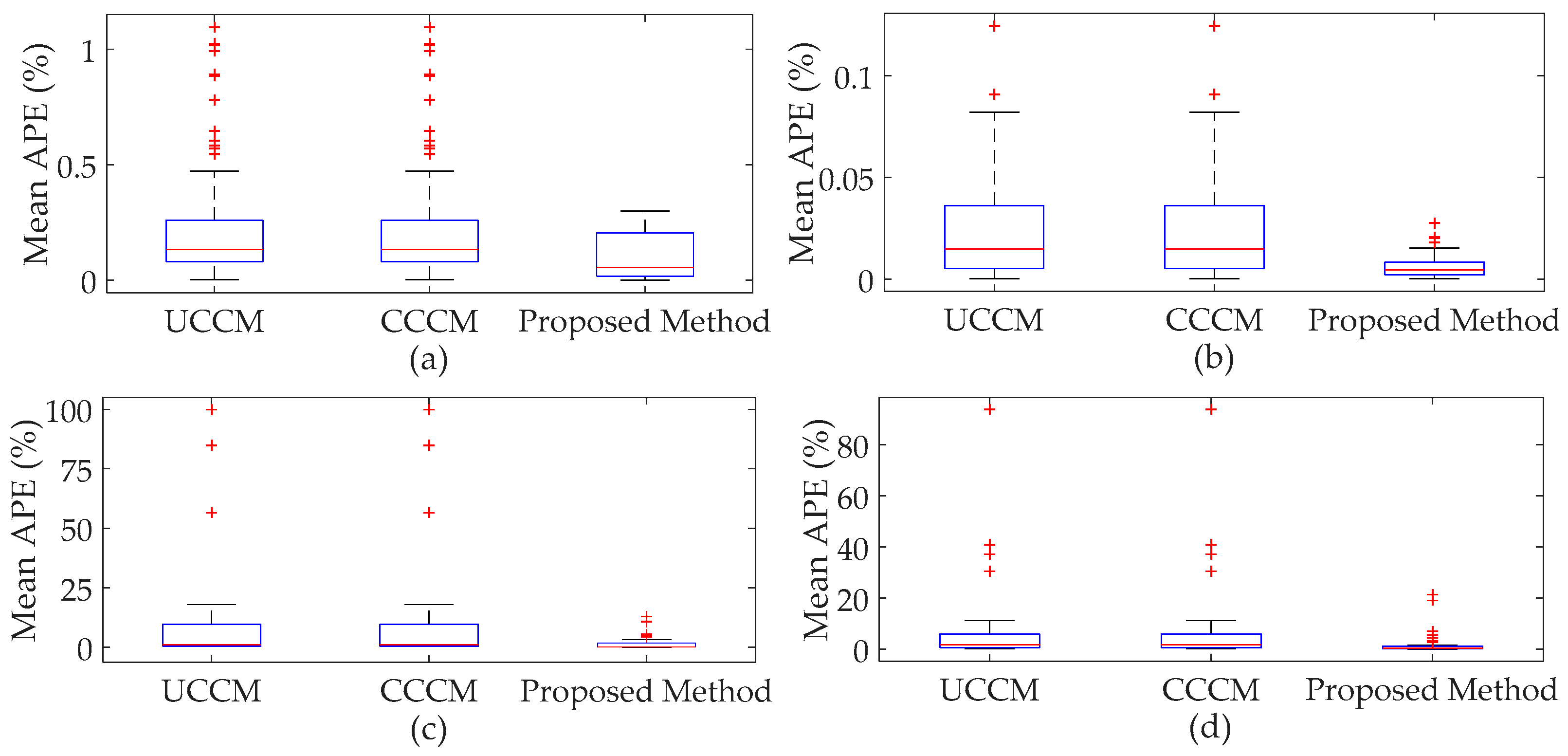
4.2. The Modified IEEE 118-Bus Test System

The IEEE 118-bus test system is modified to verify the applicability of the proposed method for a large power system with a large number of random input variables. The wind speeds are modeled as Weibull distributions with different shape and scale parameters as shown in

Table 6. Parameters of Weibull distributions (modified IEEE 118-bus test system).

Wind Speed Distribution	Shape Parameter	Scale Parameter
W1 (Connected to Bus 59)	1.732	6.611
W2 (Connected to Bus 80)	2.036	7.933
W3 (Connected to Bus 90)	1.350	5.774

[48]. As a matter of fact, there is a correlation between wind speeds at nearby wind farms, mainly due to weather conditions and locations of wind farms, etc. The closer the correlation coefficient is to either −1 or 1, the stronger the correlation between wind speeds. The correlation matrix of wind speeds is listed in

Table 7. The correlation matrix (modified IEEE 118-bus test system).

	W1	W2	W3
W1	1.00	0.76	0.64
W2	0.76	1.00	0.36
W3	0.64	0.36	1.00

. All the buses are divided into three areas, which are presented in

Table 8. Buses in each area (modified IEEE 118-bus test system).

Area	Bus Number
Area 1	1, 2, 3, 4, 5, 6, 7, 8, 9, 10, 11, 12, 13, 14, 15, 16, 17, 18, 19, 20, 21, 22, 23, 24, 25, 26, 27, 28, 29, 30, 31, 32, 113, 114, 115, 117
Area 2	33, 34, 35, 36, 37, 38, 39, 40, 41, 42, 43, 44, 45, 46, 47, 48, 49, 50, 51, 52, 53, 54, 55, 56, 57, 58, 59, 60, 61, 62, 63, 64, 65, 66, 67, 68, 69, 70, 71, 72, 73, 116
Area 3	74, 75, 76, 77, 78, 79, 80, 81, 82, 83, 84, 85, 86, 87, 88, 89, 90, 91, 92, 93, 94, 95, 96, 97, 98, 99, 100, 101, 102, 103, 104, 105, 106, 107, 108, 109, 110, 111, 112, 118

. For each area, the sum of loads follows a normal distribution with the mean value equal to the nominal value and the standard deviation equal to 10% of the mean value. The load on each bus varies with the sum of loads according to the original percentage of the sum of loads in each area, and its power factor is kept constant.

Table 9. Comparison of generation cost (modified IEEE 118-bus test system).

Algorithm	Mean	Mean APE	Standard Deviation	Standard Deviation APE
MCS	124,281.33	\	11,864.39	\
UCCM	124,093.19	0.15%	10,969.98	7.54%
CCCM	124,093.19	0.15%	11,961.51	0.82%
Proposed Method	124,244.89	0.03%	11,884.53	0.17%

shows the results obtained using different methods. It can be seen that all of the APE values obtained using the proposed method are much smaller than those obtained using UCCM and CCCM. The APE values of voltage angle, voltage magnitude, active power generation and reactive power generation are presented as box plots in Figure 7 and Figure 8. It can be seen from Figure 7 and Figure 8 that the box plots associated with the proposed method are below those associated with UCCM and CCCM, which indicates that results of the proposed method have much smaller APE values than those obtained using UCCM and CCCM. In Figure 7, for active power generation obtained using UCCM and CCCM, some mean APE values are even more than 50%. For reactive power generation obtained using UCCM and CCCM, some mean APE values exceed 20%. In Figure 8, most output variables obtained using UCCM and CCCM have large standard deviation APE values, most of which are more than 10%. These show that UCCM and CCCM are not suitable for solving the P-OPF problem with large fluctuations of stochastic variables. Figure 9 and Figure 10 show PDFs of active power generation at bus 100 and reactive power generation at bus 4. It can be seen that the curves obtained using the proposed method are closer to the MCS histograms than those obtained using UCCM and CCCM, especially at the tails of curves. For other system variables, similar results can be obtained.

Meanwhile, the computation time using the proposed method is about dozens of times less than that using MCS, as shown in

Table 10. Computation time table for the modified IEEE 118-bus test system.

Algorithm	Time (s)
MCS	6195.28
UCCM	13.24
CCCM	13.46
Proposed Method	171.48

. It should be pointed out that the proposed method takes more time than UCCM and CCCM. That is because the proposed method conducts P-OPF many times according to the number of clusters, and UCCM and CCCM only conduct P-OPF once. For the proposed method, the number of calculations depends on the distributions and correlations of stochastic variables, as well as the accuracy requirements (discussed in Section 4.3). The proposed method is superior in view of the fact that UCCM and CCCM cannot handle large fluctuations of input variables. In summary, the proposed method performs better, based on the accuracy, than traditional CM and requires much less computation time than MCS.

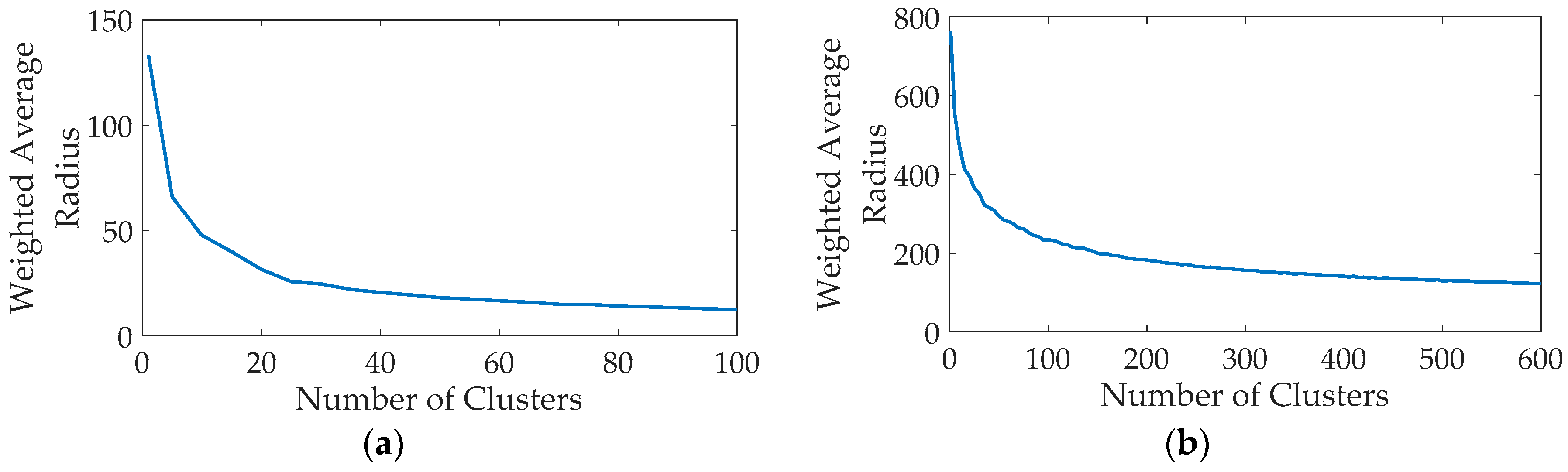
4.3. Discussions about Number of Clusters

It is obvious that the proposed method with more clusters generally has better performance, based on the accuracy, at the expense of time. Therefore, it is desirable to select an appropriate number of clusters for the proposed method, which has acceptable accuracy and computation time.

The appropriate number of clusters can be obtained by measuring the performance of K-means. The weighted average radius is proposed to measure the performance of clustering:

$$R={\displaystyle \sum }_{i=1}^k{p}_i\times r_i$$

(21)

where $R$ is the weighted average radius, $p_i$ is the proportion of the number of elements in cluster $i$ to the total samples, and $r_i$ is the radius of cluster $i$ [43].

Figure 11 shows the relation curves between weighted average radius and number of clusters for the above two cases. It can be observed that the curve for the modified IEEE 9-bus test system changes very slowly, when the number of clusters exceeds 25. Similarly, the curve for the modified IEEE 118-bus test system changes very slowly, when the number of clusters exceeds 100. Therefore, the appropriate values of $k$ for the modified IEEE 9-bus and 118-bus test system are suggested to be 25 and 100, respectively.

As discussed in Section 4.1 and Section 4.2, the proposed method with the suggested value of $k$ performs well, based on the accuracy and computation time. If decision makers want to get more accurate results, a larger value of $k$ should be selected. For example, for the modified IEEE 9-bus test system, the mean APE value of reactive power at bus 2 is improved from 11.75% to 7.81% by the proposed method with 50 clusters.

5. Conclusions

This paper proposes a novel method to solve P-OPF problems with consideration of correlations and large fluctuations of stochastic variables, which can be applied to power systems with large-scale wind power integration. In the process, the K-means algorithm is introduced to group input variables into a number of clusters. In order to obtain the moments for the total samples, the total probability formula is used to combine the moments computed in each cluster using CM. IEEE 9-bus and 118-bus test systems are modified to analyze the performance of the proposed method. It should be pointed out that the historical data of wind speeds and loads can be directly used for clustering, and the samples of wind speeds and loads will not need to be generated. Some conclusions are summarized as follows:

• When input variables have large fluctuations, P-OPF results obtained using the traditional CM have large APE values and significant errors at the tails of PDFs, which indicates that the traditional CM is not suitable to solve P-OPF problems with large fluctuations of stochastic variables.
• The proposed method can handle correlations and large fluctuations of input variables. Case studies indicate that the proposed method has more accurate results than traditional CM and is more efficient than MCS.
• The performance of the proposed method is influenced by the number of clusters. Generally, the proposed method with more clusters has more accurate results, but will require more computation time. The appropriate number of clusters can be determined by the weighted average radius.

References

1. Momoh, J.A.; Koessler, R.J.; Bond, M.S.; Stott, B.; Sun, D.; Papalexopoulos, A.; Ristanovic, P. Challenges to optimal power flow. IEEE Trans. Power Syst. 1997, 12, 444–455. [Google Scholar] [CrossRef]
2. Huneault, M.; Galiana, F.D. A survey of the optimal power flow literature. IEEE Trans. Power Syst. 1991, 6, 762–770. [Google Scholar] [CrossRef]
3. Huang, C.M.; Kuo, C.J.; Huang, Y.C. Short-term wind power forecasting and uncertainty analysis using a hybrid intelligent method. IET Renew. Power Gener. 2017, 11, 678–687. [Google Scholar] [CrossRef]
4. Ellis, A.; Schoenwald, D.; Hawkins, J.; Willard, S.; Arellano, B. PV output smoothing with energy storage. In Proceedings of the 2012 38th IEEE Photovoltaic Specialists Conference, Austin, TX, USA, 3–8 June 2012. [Google Scholar]
5. Aien, M.; Rashidinejad, M.; Firuz-Abad, M.F. Probabilistic optimal power flow in correlated hybrid wind-PV power systems: A review and a new approach. Renew. Sustain. Energy Rev. 2015, 41, 1437–1446. [Google Scholar] [CrossRef]
6. Prusty, B.R.; Jena, D. A critical review on probabilistic load flow studies in uncertainty constrained power systems with photovoltaic generation and a new approach. Renew. Sustain. Energy Rev. 2017, 69, 1286–1302. [Google Scholar] [CrossRef]
7. Zhang, H.; Li, P. Probabilistic analysis for optimal power flow under uncertainty. IET Gener. Transm. Distrib. 2010, 4, 553–561. [Google Scholar] [CrossRef]
8. Cao, J.; Yan, Z. Probabilistic optimal power flow considering dependences of wind speed among wind farms by pair-copula method. Int. J. Electr. Power 2017, 84, 296–307. [Google Scholar] [CrossRef]
9. Rubinstein, R.Y.; Kroese, D.P. Simulation and the Monte Carlo Method, 2nd ed.; John Wiley & Sons, Inc.: Hoboken, NJ, USA, 2007. [Google Scholar]
10. Gentle, J.E. Random Number Generation and Monte Carlo Methods, 2nd ed.; Springer: New York, NY, USA, 2003. [Google Scholar]
11. Huang, J.; Xue, Y.; Dong, Z.Y.; Wong, K.P. An adaptive importance sampling method for probabilistic optimal power flow. In Proceedings of the 2011 IEEE Power and Energy Society General Meeting, Detroit, MI, USA, 24–29 July 2011; pp. 1–6. [Google Scholar]
12. Gang, L.; Jinfu, C.; Defu, C.; Dongyuan, S.; Xianzhong, D. Probabilistic assessment of available transfer capability considering spatial correlation in wind power integrated system. IET Gener. Transm. Distrib. 2013, 7, 1527–1535. [Google Scholar] [CrossRef]
13. Yu, H.; Chung, C.Y.; Wong, K.P.; Lee, H.W.; Zhang, J.H. Probabilistic Load Flow Evaluation with Hybrid Latin Hypercube Sampling and Cholesky Decomposition. IEEE Trans. Power Syst. 2009, 24, 661–667. [Google Scholar] [CrossRef]
14. Hajian, M.; Rosehart, W.D.; Zareipour, H. Probabilistic Power Flow by Monte Carlo Simulation with Latin Supercube Sampling. IEEE Trans. Power Syst. 2013, 28, 1550–1559. [Google Scholar] [CrossRef]
15. Xie, Z.Q.; Ji, T.Y.; Li, M.S.; Wu, Q.H. Quasi-Monte Carlo Based Probabilistic Optimal Power Flow Considering the Correlation of Wind Speeds Using Copula Function. IEEE Trans. Power Syst. 2017, 1. [Google Scholar] [CrossRef]
16. Zou, B.; Xiao, Q. Solving Probabilistic Optimal Power Flow Problem Using Quasi Monte Carlo Method and Ninth-Order Polynomial Normal Transformation. IEEE Trans. Power Syst. 2014, 29, 300–306. [Google Scholar] [CrossRef]
17. Prasad, C.B.; Chintham, V. Probabilistic Optimal Power Flow with wind energy penetration and integration of storage system. In Proceedings of the 2015 Annual IEEE India Conference (INDICON), New Delhi, India, 17–20 December 2015; pp. 1–6. [Google Scholar]
18. Verbic, G.; Canizares, C.A. Probabilistic Optimal Power Flow in Electricity Markets Based on a Two-Point Estimate Method. IEEE Trans. Power Syst. 2006, 21, 1883–1893. [Google Scholar] [CrossRef]
19. Arabali, A.; Ghofrani, M.; Etezadi-Amoli, M. Cost analysis of a power system using probabilistic optimal power flow with energy storage integration and wind generation. Int. J. Electr. Power 2013, 53, 832–841. [Google Scholar] [CrossRef]
20. Morales, J.M.; Perez-Ruiz, J. Point Estimate Schemes to Solve the Probabilistic Power Flow. IEEE Trans. Power Syst. 2007, 22, 1594–1601. [Google Scholar] [CrossRef]
21. Sebastián, G.-C.J.; Alexander, C.-L.J.; Mauricio, G.-E. Stochastic AC Optimal Power Flow Considering the Probabilistic Behavior of the Wind, Loads and Line Parameters. Ing. Investig. Tecnol. 2014, 15, 529–538. [Google Scholar] [CrossRef]
22. Li, X.; Cao, J.; Du, D. Probabilistic optimal power flow for power systems considering wind uncertainty and load correlation. Neurocomputing 2015, 148, 240–247. [Google Scholar] [CrossRef]
23. Morales, J.M.; Baringo, L.; Conejo, A.J.; Minguez, R. Probabilistic power flow with correlated wind sources. IET Gener. Transm. Distrib. 2010, 4, 641–651. [Google Scholar] [CrossRef]
24. Wang, X.; Gong, Y.; Jiang, C. Regional Carbon Emission Management Based on Probabilistic Power Flow with Correlated Stochastic Variables. IEEE Trans. Power Syst. 2015, 30, 1094–1103. [Google Scholar] [CrossRef]
25. Li, Y.; Li, W.; Yan, W.; Yu, J.; Zhao, X. Probabilistic Optimal Power Flow Considering Correlations of Wind Speeds Following Different Distributions. IEEE Trans. Power Syst. 2014, 29, 1847–1854. [Google Scholar] [CrossRef]
26. Shargh, S.; Khorshid ghazani, B.; Mohammadi-ivatloo, B.; Seyedi, H.; Abapour, M. Probabilistic multi-objective optimal power flow considering correlated wind power and load uncertainties. Renew. Energy 2016, 94, 10–21. [Google Scholar] [CrossRef]
27. Xia, S.; Luo, X.; Chan, K.W.; Zhou, M.; Li, G. Probabilistic Transient Stability Constrained Optimal Power Flow for Power Systems with Multiple Correlated Uncertain Wind Generations. IEEE Trans. Sustain. Energy 2016, 7, 1133–1144. [Google Scholar] [CrossRef]
28. Aien, M.; Fotuhi-Firuzabad, M.; Aminifar, F. Probabilistic Load Flow in Correlated Uncertain Environment Using Unscented Transformation. IEEE Trans. Power Syst. 2012, 27, 2233–2241. [Google Scholar] [CrossRef]
29. Valverde, G.; Saric, A.T.; Terzija, V. Probabilistic load flow with non-gaussian correlated random variables using gaussian mixture models. IET Gener. Transm. Distrib. 2012, 6, 701–709. [Google Scholar] [CrossRef]
30. Pei, Z.; Lee, S.T. Probabilistic load flow computation using the method of combined cumulants and Gram-Charlier expansion. IEEE Trans. Power Syst. 2004, 19, 676–682. [Google Scholar]
31. Fan, M.; Vittal, V.; Heydt, G.T.; Ayyanar, R. Probabilistic Power Flow Studies for Transmission Systems with Photovoltaic Generation Using Cumulants. IEEE Trans. Power Syst. 2012, 27, 2251–2261. [Google Scholar] [CrossRef]
32. Yuan, Y.; Zhou, J.; Ju, P.; Feuchtwang, J. Probabilistic load flow computation of a power system containing wind farms using the method of combined cumulants and Gram-Charlier expansion. IET Renew. Power Gener. 2011, 5, 448–454. [Google Scholar] [CrossRef]
33. Cai, D.; Chen, J.; Shi, D.; Duan, X.; Li, H.; Yao, M. Enhancements to the Cumulant Method for probabilistic load flow studies. In Proceedings of the 2012 IEEE Power and Energy Society General Meeting, San Diego, CA, USA, 22–26 July 2012; pp. 1–8. [Google Scholar]
34. Ran, X.; Miao, S. Three-phase probabilistic load flow for power system with correlated wind, photovoltaic and load. IET Gener. Transm. Distrib. 2016, 10, 3093–3101. [Google Scholar] [CrossRef]
35. Prusty, B.R.; Jena, D. Combined cumulant and Gaussian mixture approximation for correlated probabilistic load flow studies: A new approach. CSEE J. Power Energy Syst. 2016, 2, 71–78. [Google Scholar] [CrossRef]
36. Schellenberg, A.; Rosehart, W.; Aguado, J. Cumulant-based probabilistic optimal power flow (P-OPF) with Gaussian and gamma distributions. IEEE Trans. Power Syst. 2005, 20, 773–781. [Google Scholar] [CrossRef]
37. Tamtum, A.; Schellenberg, A.; Rosehart, W.D. Enhancements to the Cumulant Method for Probabilistic Optimal Power Flow Studies. IEEE Trans. Power Syst. 2009, 24, 1739–1746. [Google Scholar] [CrossRef]
38. Allan, R.N.; Silva, A.M.L.D.; Burchett, R.C. Evaluation Methods and Accuracy in Probabilistic Load Flow Solutions. IEEE Trans. Power Appl. Syst. 1981, PAS-100, 2539–2546. [Google Scholar] [CrossRef]
39. Torres, G.L.; Quintana, V.H. Optimal power flow via interior point methods: An educational tool in Matlab. In Proceedings of the 1996 Canadian Conference on Electrical and Computer Engineering, Calgary, AB, Canada, 26–29 May 1996; Volume 2, pp. 996–999. [Google Scholar]
40. Giorsetto, P.; Utsurogi, K.F. Development of a New Procedure for Reliability Modeling of Wind Turbine Generators. IEEE Trans. Power Appl. Syst. 1983, PAS-102, 134–143. [Google Scholar] [CrossRef]
41. Qin, Z.; Li, W.; Xiong, X. Generation System Reliability Evaluation Incorporating Correlations of Wind Speeds with Different Distributions. IEEE Trans. Power Syst. 2013, 28, 551–558. [Google Scholar] [CrossRef]
42. Usaola, J. Probabilistic load flow in systems with wind generation. IET Gener. Transm. Distrib. 2009, 3, 1031–1041. [Google Scholar] [CrossRef] [Green Version]
43. Rajaraman, A.; Leskovec, J.; Ullman, J.D. Mining of Massive Datasets; Cambridge University Press: Cambridge, UK, 2012. [Google Scholar]
44. Liu, J.; Hao, X.; Cheng, P.; Fang, W.; Niu, S. A Parallel Probabilistic Load Flow Method Considering Nodal Correlations. Energies 2016, 9, 1041. [Google Scholar] [CrossRef]
45. Papoulis, A.; Pillai, S.U. Probability, Random Variables, and Stochastic Processes, 4th ed.; McGraw-Hill: New York, NY, USA, 2002. [Google Scholar]
46. MATPOWER. Available online: http://www.pserc.cornell.edu/matpower/ (accessed on 7 January 2017).
47. Aien, M.; Fotuhi-Firuzabad, M.; Rashidinejad, M. Probabilistic Optimal Power Flow in Correlated Hybrid Wind-Photovoltaic Power Systems. IEEE Trans. Smart Grid 2014, 5, 130–138. [Google Scholar] [CrossRef]
48. Masseran, N.; Razali, A.M.; Ibrahim, K. An analysis of wind power density derived from several wind speed density functions: The regional assessment on wind power in Malaysia. Renew. Sustain. Energy Rev. 2012, 16, 6476–6487. [Google Scholar] [CrossRef]
Figure 1. The flowchart of the proposed method.
Energies 10 01623 g001
Figure 2. The elements of the samples of wind power outputs and loads.
Energies 10 01623 g002
Figure 3. Comparison of APE values of generators’ reactive power (modified IEEE 9-bus test system). (a) Mean APE values; (b) Standard deviation APE values.
Energies 10 01623 g003
Figure 4. Comparison of APE values of voltage magnitude at each bus (modified IEEE 9-bus test system). (a) Mean APE values; (b) Standard deviation APE values.
Energies 10 01623 g004aEnergies 10 01623 g004b
Figure 5. PDFs of generation cost (modified IEEE 9-bus test system).
Energies 10 01623 g005
Figure 6. PDFs of reactive power generation at bus 2 (modified IEEE 9-bus test system).
Energies 10 01623 g006
Figure 7. Box plot of mean APE of results (modified IEEE 118-bus test system). (a) Voltage angle; (b) Voltage magnitude; (c) Active power generation; (d) Reactive power generation.
Energies 10 01623 g007
Figure 8. Box plot of standard deviation APE of results (modified IEEE 118-bus test system). (a) Voltage angle; (b) Voltage magnitude; (c) Active power generation; (d) Reactive power generation.
Energies 10 01623 g008
Figure 9. PDFs of active power generation at bus 100 (modified IEEE 118-bus test system).
Energies 10 01623 g009
Figure 10. PDFs of reactive power generation at bus 4 (modified IEEE 118-bus test system).
Energies 10 01623 g010
Figure 11. Relation curves between weighted average radius and number of clusters. (a) Modified IEEE 9-bus test system; (b) Modified IEEE 118-bus test system.
Energies 10 01623 g011