Abstract
Eye movements are an important cue to understand consumer decision processes. Findings from existing studies suggest that the consumer decision process consists of a few different browsing states such as screening and evaluation. This study proposes a hidden Markov-based gaze model to reveal the characteristics and temporal changes of browsing states in catalog browsing situations. Unlike previous models that employ a heuristic rule-based approach, our model learns the browsing states in a bottom-up manner. Our model employs information about how often a decision maker looks at a selected item (the item finally selected by a decision maker) to identify the browsing states. We evaluated our model using eye tracking data in catalog browsing and confirmed our model can split decision process into meaningful browsing states. Finally, we propose an estimation method of browsing states that does not require the information of the selected item for applications such as an interactive decision support.
Introduction
Understanding cognitive processes in decision making has been a target of research for the past several decades (Payne, 1976). Human eye movements are a powerful measurement that helps researchers understand how people obtain and process information of alternative choices and recent development of eye tracking devices has contributed to this research topic (Orquin & Loose, 2013). Compared to other traditional process tracing methods (think-out-loud (Payne, 1976) or MouseLab (Payne, Bettman, & Johnson, 1993)), eye movements have a distinct advantage that they can be recorded with higher sampling rates and with fewer cognitive impacts. Various aspects of decision making have been investigated using eye tracking data, including viewers’ preference (Sugano, Ozaki, Kasai, & Ogaki, 2014; Shimojo, Simion, Shimojo, & Scheier, 2003), decision tasks (Pfeiffer, Meißner, Prosiegel, & Pfeiffer, 2014), and motivations and time pressure (Pieters & Warlop, 1999).
The advantage of tracking eye movements enables the detailed analysis of decision processes including the temporal changes of cognitive states of decision makers. Several studies have shown that the decision process consists of a few different phases (Orquin & Loose, 2013), that is, decision makers split their decision making task into smaller sub-tasks such as the screening of alternatives. These phases are sometimes referred to as decision stages (Russo & Leclerc, 1994; Gidlöf, Wallin, Dewhurst, & Holmqvist, 2013) or attention phases (Orquin & Loose, 2013). In this work, the term “decision stages” is used. The existence of decision stages has been confirmed in many works (Russo & Leclerc, 1994; Wedell & Senter, 1997; Clement, 2007; Glaholt & Reingold, 2011; Reutskaja, Nagel, Camerer, & Rangel, 2011; Glöckner & Herbold, 2011; Gidlöf et al., 2013).
In early versions of decision stage models, before eye tracking was widely used, the decision process was considered to be roughly separated into two types of decision stages: screening and evaluation (Payne, 1976). In the screening stage, decision makers obtain an overview of information of all products; then, in the evaluation stage, they evaluate the few remaining alternatives to make a selection. To our knowledge, Russo et al. were the first to utilize eye tracking to model decision stages (Russo & Rosen, 1975; Russo & Leclerc, 1994). Russo measured participants’ eye movements in a supermarket-like experimental environment where real products were displayed on a shelf. Through the experiment, Russo et al. confirmed the existence of a verification stage after the two previously proposed decision stages. Their work lead to a lot of follow-up work on decision stages in decision making (Wedell & Senter, 1997; Clement, 2007; Glaholt & Reingold, 2011; Reutskaja et al., 2011; Glöckner & Herbold, 2011; Gidlöf et al., 2013).
Many questions still remain in decision stage analysis; a fundamental problem is that there is no concrete method for identification of decision stages. Existing methods employ a heuristic approach in which top-down rules are given by analysts based on their observations. This caused disagreement among the previous studies, such as the number of decision stages and their interpretations. Some studies (Gidlöf et al., 2013; Russo & Leclerc, 1994) noted the decision stages cannot be clearly separated like the previous studies assumed. The boundary between stages is further blurred due to the occasional interruption into other stages. For example, it is likely for decision makers to go back to the screening stage to re-input item information during the evaluation stage. Thus, a concrete theory on the quantity and type of decision stages is not established, and this may change with task characteristics. Accordingly, it is not feasible to model the decision stage interruptions by defining top-down rules that cover all possible cases.
In this paper, we propose a choice behavior model to trace the temporal changes of decision stages in consumer decision process based on a probabilistic approach. Unlike previous top-down approaches, the probabilistic model presented here learns the segments of stages using eye tracking data in a bottom-up manner, which means we do not have to know about the details of decision stages or how they transit a priori. We exploit only a couple of simple assumptions about interval lengths between a glance and the next glance on the selected item (the alternative finally selected by the decision maker), and the rest of the model (including how stages transit) is learned from the data. In order to deal with bidirectional transitions between stages described above, we use a hidden Markov model whose state corresponds to decision stages. Here, the decision stages of our model are referred to as browsing states to represent their bidirectional characteristics instead of the term of stage that indicates unidirectional transitions. Our method is evaluated through an eye tracking experiment in a digital catalog browsing situation with experimenter-specified task criterion. The task criterion specifies the number of candidates among a set of items on a screen. Then, our approach was evaluated by measuring how the model can segment reasonable intervals for browsing states in terms of (1) description capability of differences among the tasks and (2) accuracy in identifying when a participant is exhibiting comparison behavior among candidate items.
The proposed browsing model enables more detailed analysis of decision stages, such as how the interruptions of stages relate to decision tasks. It is also possible to use our model for applications such as interactive information systems that support human decision making by providing the right information at the right time. In this situation, the information about selected items that our model uses to identify browsing states is not available. Thus, we also propose an estimation method of browsing states that only requires eye tracking data and content layout information. To achieve this, our choice behavior model is extended to a hidden semiMarkov model (Yu, 2010) so that it can describe duration of browsing states. The estimation method is evaluated by measuring how it can replicate the results by our model that uses information of the selected item.
Consumer Decision Processes
This section first presents more detail on previously proposed decision stage models and their limitations (Russo & Leclerc, 1994; Gidlöf et al., 2013). Next, we present several existing information search gaze models that take a probabilistic approach. Finally, we introduce findings on browsing behavior in different task complexities.
Catalog Browsing States
Russo et al. pioneered decision stage analysis using eye tracking (Russo & Leclerc, 1994). They investigated the existence of decision stages in consumer decision processes and their characteristics. As a result of their eye tracking experiments, they found that the decision processes consist of three stages: orientation, evaluation, and verification. In their paper, each stage is identified based on a sequence of “dwells” on alternative items, where a dwell here is a set of consecutive fixations on each alternative (The term of ‘fixation’ here indicates a visual fixation between saccades. The term is also used in Russo’s paper (Russo & Leclerc, 1994), however, Russo’s “fixation” corresponds to a glance or a dwell in this paper). Dwell sequence analysis is the commonly used approach for process tracing of decision stages (Glaholt & Reingold, 2011; Orquin & Loose, 2013). The orientation stage is defined to be the stage that occurs before the first “re-dwell” (a dwell on an alreadyexamined item) appears. The evaluation stage is between the first and the last re-dwell and the verification stage is after the last re-dwell. This study leads to a lot of follow-up work on decision stage analysis; however, the validity of Russo’s work has been questioned by some researchers due to the fact that the researchers were manually tracking participants’ eye movements through a one-way mirror (Pfeiffer et al., 2014). More recently, Gidlöf et al. re-evaluated Russo’s threestage model, calling it the Natural Decision Segmentation Model (NDSM), and used modern eye tracking technology (Gidlöf et al., 2013). In NDSM, the information of the selected item is used as a stage divider, i.e., the evaluation stage in NDSM is defined to be between the first and the last dwell on the selected item. Their model was evaluated through a real-world super market experiment by measuring how the identified decision stages can describe differences between two tasks (search and decision) compared to Russo’s model. Their research established a difference in browsing behavior between the two tasks, however, their method of identifying different decision stages still had some limitations. As noted in their paper, the stages can be often interrupted by other stages, for example, going back to the orientation stage to re-input item information during the evaluation stage. Instead of defining rules to cover the interruption of decision stages, Gidlöf et al. assumed each stage is dominated by a specific function of the decision process even if it contains elements of other stages.
Ideally, decision stage analysis would account for the interruption of stages; however, it is not possible to define top-down rules that cover all situations. This is because the needed information about browsing states is not known in advance, i.e., the number of stages that appear in a decision making session and possible types of decision stages can vary depending on decision making factors such as tasks, user personalities, and so on.
Probabilistic approach in modeling information processing states
Groner et al. pioneered modeling of human information processing based on Markov models (Groner & Spada, 1977; Groner & Groner, 1982, 1983). They empirically showed that their proposed models can predict eye movements and error patterns in high-level cognitive process such as problem solving. Liechty et al. proposed a hidden Markov model to capture two distinct attention states (local or global) while visually exploring complex scenes (Liechty, Pieters, & Wedel, 2003). In the local search state, viewers focus on specific aspects and details of the scene, meanwhile, in the global attention state, viewers focus on exploring the informative and perceptually salient areas of the scene. Their model is evaluated through an eye tracking experiment of consumers’ attention to print advertisements in magazines. Simola et al. (Simola, Salojärvi, & Kojo, 2008) employed a HMM to uncover processing states in text reading. Three HMMs were built using sequences of gaze motion features (e.g., saccade lengths) corresponding to three different information-search tasks: simple word search, finding the answer to a question, and selecting an interesting title from a list. Their results showed that the tasks can be estimated from a newly observed sequence of eye movements by comparing the likelihood of each model. In their model, hidden states are learned using gaze data without any prior knowledge, and are interpreted as scanning, reading, and decision.
There are a few probabilistic gaze models in consumer decision process. Stüttgen et al. proposed a satisfactory decision process model using eye tracking data (Stüttgen, Boatwright, & Monroe, 2012). The satisfactory decision process model is a decision making model that assumes decision makers choose alternatives that satisfy a set of specific criteria. In their model, information search behavior is represented by a HMM which has two states: local and global search state based on the above mentioned Liechty’s local/global attention model (Liechty et al., 2003). Shi et al. proposed a hierarchical HMM to uncover information acquisition process on catalogs with attribute-by-product matrix layouts (Shi, Wedel, & Pieters, 2013). Their model consists of two layers of hidden states, in which the lower layer hidden states correspond to types of information acquisition processes, and the higher layer hidden states correspond to strategy. For their model observations, they employ probabilities of three of the types of transitions among AOIs (regions that describe an attribute of a product) on a screen: attribute-based (a transition between regions of the same attribute but different items), product-based (a transition between regions of different attributes but for the same item), and others. Although their model can represent similar states to decision stages, it can be applied to only eye movements for catalogs with attribute-by-product matrix layouts. In most situations where the differences between attributebased and product-based information search behavior are unclear, we need to reconsider which features of gaze should be analyzed.
Browsing states and task complexities
Information processing varies with the parameters of decision making tasks (Payne, 1976). When people are faced with a decision between two alternatives, they employ a compensatory decision process in which all available information of alternatives is considered together to make a comprehensive decision. In contrast, when people face a more difficult decision task (with more alternatives), they tend to employ a non-compensatory decision process in which some of the available alternatives are eliminated quickly based on some specific criteria (e.g., filtering). After narrowing the alternatives down, people finally evaluate the alternatives using a compensatory decision process. This is simply because of a limited information processing capability of decision makers. Note that the compensatory decision process corresponds to the evaluation state in our model.
Approach of this study
As discussed above, there are two main issues when modeling temporal changes of browsing states that correspond to decision stages in the consumer decision process: (1) managing the diversity of browsing states and (2) characterizing features of gaze for identifying the browsing states. To address the issue (1), this work provides a bottom-up framework in which probabilistic relations between decision stage and gaze behavior are learned from recorded gaze data. A hidden Markov model (HMM) was employed to represent transitions among browsing states. To address the issue (2), we proposed a methodology for browsing-state identification that can be used in the situation where we only know when the selected item is looked at in the transitions of gaze target items.
Our approach was evaluated by measuring the description capability of differences among tasks. Here, we assume that the number of remaining alternatives (after the eliminating process) affects the temporal duration of the evaluation state. Ideally, if our assumption is correct and if only one alternative remains after screening, the evaluation state would not be observed. Meanwhile, if multiple alternatives (strong candidates) remain after screening, the duration of the evaluation state would increase.
Data Collection
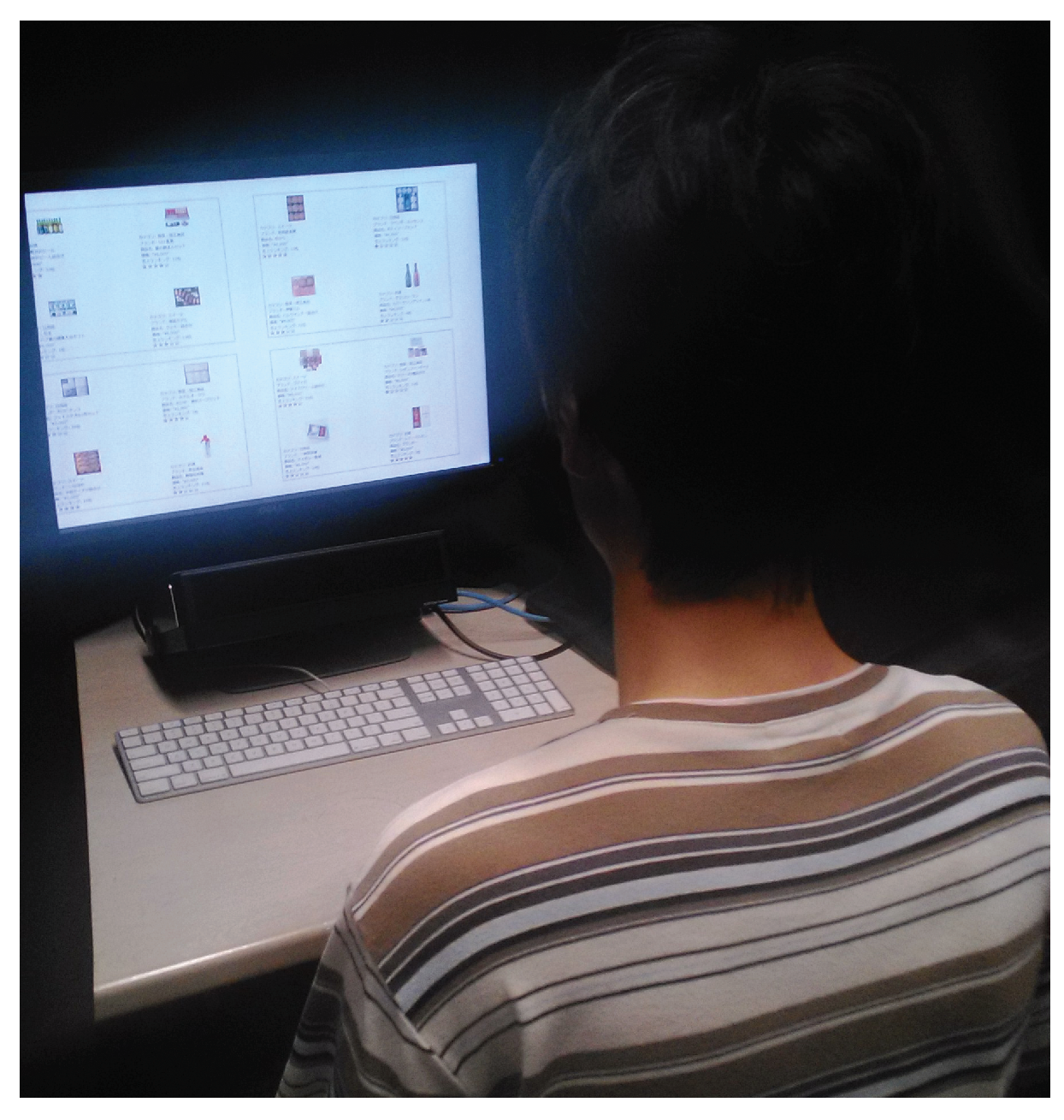
Eight participants took part in the experiment. Each participant was asked to sit in front of a display showing a digital catalog (see Figure 1a). Gaze data of the participants were acquired as 2D points on the display by using an eye tracker (Tobii X120 (freedom of head movement: 400x220x300 mm, sampling rate: 60 Hz, accuracy: 0.5 degrees)) installed below the display.

Figure 1.
Experimental environment. A participant is browsing a digital catalog on a display. Gaze data of the participant are recorded by the eye tracker installed below the display.
Digital catalogs
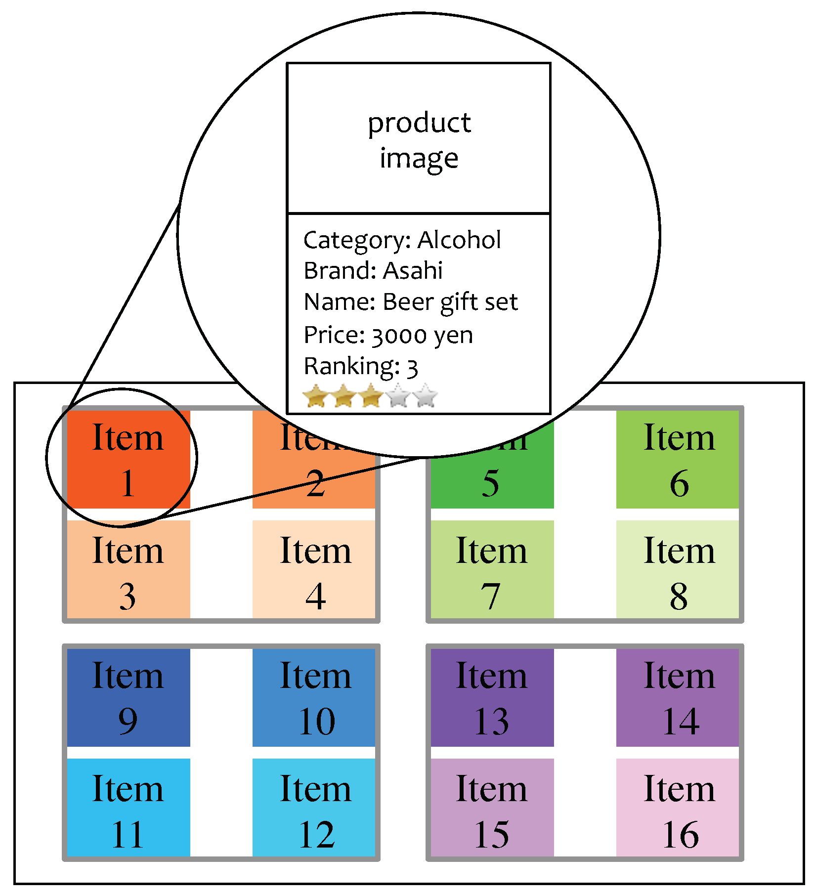
For each participant, eight digital catalogs were prepared. Each digital catalog contained the description (images and text) of 16 items (see Figure 2). The semantic attributes and attribute values of items that were available in this study are listed in Table 1. The semantic information was described in text on the catalogs so that viewers could understand it without prior knowledge. The items in each catalog were grouped by either price or category attribute. The item positions within a group were randomized every time the catalog was shown to a participant.
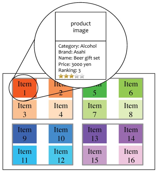
Figure 2.
Layout of digital catalogs. Items with a same color hue are in a same group, and each group of items are divided by a gray frame.

Table 1.
The attributes and attribute values used in the experiments.
Task complexity
Participants were asked to select an item from a catalog as a seasonal gift. Without any experimental manipulation, the selection situation would vary based on participants’ preference and products in catalogs. For example, it is possible that participants make a decision among multiple strong candidates, or perhaps they can find only one product that satisfies their criteria. Since it is difficult to obtain such information, we gave participants a request that specified the requirements for items to select for each trial, for example: “Select an item in the Alcohol category and with more than a 4-star review." In previous work done by Pfeiffer et al., they noted goaldirected search behavior can be induced in participants during in-store experiments by fixing requests so that only one item in the store satisfies all of the conditions (Pfeiffer et al., 2014). We take a similar approach here; however, we change the number of items that satisfy the requests to be between 0 to 3 to investigate the relations between browsing states and task complexities. In the rest of this paper, the term of candidates is used to indicate items that satisfy the request. The number of gaze sequences recorded in the experiments with each condition of task complexity (number of candidates) is shown in Table 2. We discarded gaze sequences in which a participant chose an item that did not satisfy the given request (even though at least one candidate existed in the catalog).
Table 2.
The number of gaze sequences with each task complexity.
Procedure
The first decision making session of each participant started with a short, 5-point calibration phase. Each participant performed eight decision making sessions. In each session, one of the requests was shown to the participant before showing the catalog. The participants were instructed to follow the request to the best of their ability. During catalog browsing, the participants were able to refer to the request by pressing the space key on a provided keyboard in case where they forget the request. The gaze data during catalog browsing were registered together with the time stamps when the space key was pressed. The participants were instructed to press the enter key on the keyboard when they made a decision. When the enter key was pressed, the catalog on the monitor was suddenly hidden. After the catalog was hidden, the participant was asked to name the selected item.
Examples of collected gaze data
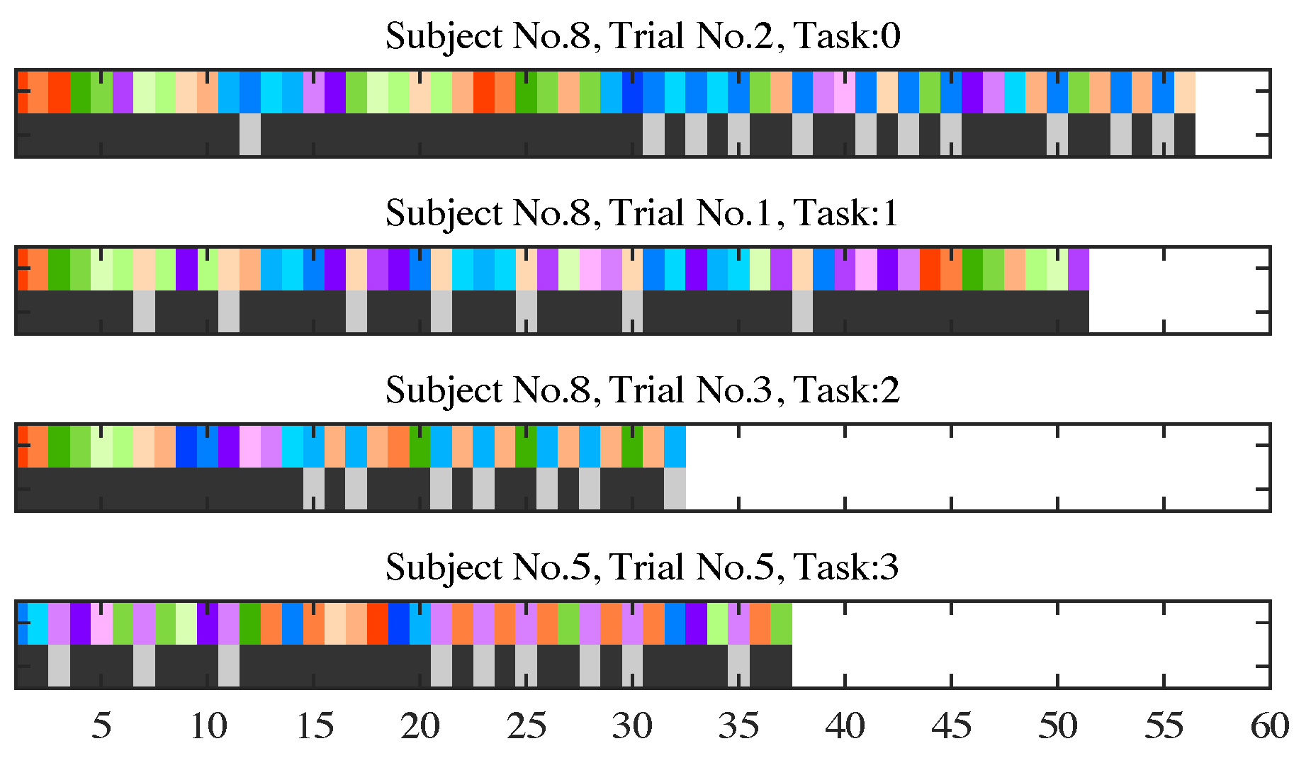
The average of the tracking loss rates in each gaze sequence was 6.95%. Eye trackers sometimes contain noise in participants’ eye movements, which can make analysis difficult. To manage error, our recorded sequences of sampling points were first smoothed by applying a median filter (In this paper, the window size of the median filter was 5 sampling points at 60 Hz (corresponding to about 83 msec)). For the subsequent analysis, each sequence of sampling points was first converted to a sequence of dwells on items. Recall that a dwell is a set of successive samples in each area of interest (AOI), and the dwell sequence analysis is often used in previous studies on consumer decision analysis (Glaholt & Reingold, 2011). In this study, AOIs are the regions of items and each dwell is simply identified by a set of successive sampling points in each item region without identifying fixations. The dwell sequences are modified by discarding dwells with duration shorter than a threshold (100 msec). Moreover, if successive dwells with the same item ID were interrupted by a blink, the intervals were combined to a longer dwell. Any dwell in which the participant was referring to the requirements of the request was also discarded. Examples of dwell sequences are shown in Figure 3. In the examples, we can observe temporal differences of the frequency of dwells on a selected item. In the top and the third examples, similar behavior to the gaze cascade effect (Shimojo et al., 2003) can be confirmed. That is, the selected items are more frequently looked at as time progresses. The second example supports the assertion by Russo et al. (Russo & Leclerc, 1994). We can see an exploratory browsing behavior after the 38th dwell on the selected item, which can be interpreted as the verification stage. The bottom example highlights the importance of considering probabilistic transitions between decision stages. In the bottom example, there is an interval that contains fewer dwells on the selected item from the 12th dwell to the 20th dwell. Considering whether or not each item has been looked at, this example may be interpreted as follows: the participant was exploring the catalog until the 20th dwell with the interruption of evaluating behavior occurring at the beginning.

Figure 3.
Example of dwell sequences. The horizontal axis shows the index of dwells. For each sequence, the color in the top row corresponds to the color of regions in Figure 2, and the bottom row shows the timings of dwells on the selected item by light gray highlights.
Proposed Model
This section describes the details of the proposed choice behavior model and the results of its evaluation. First, basic assumptions about the browsing states are described. Next, we explain how we formulate the assumptions for the probabilistic model. Finally, our browsing model is evaluated using eye tracking data collected in the previous section.
The basic assumption of browsing states
Here we make a couple of assumptions of browsing states in multi-alternative choice situations. First, we assume the consumer decision process can be described by two types of browsing states: exploration and evaluation. The exploration state is a decision state where decision makers aim to obtain broad information of items to screen items out or to confirm their decision. Meanwhile, the evaluation state is a decision state where a decision maker aims to obtain detailed information of fewer items to evaluate them as strong candidates. We define the correspondence between our browsing states and the three decision stages in the previously proposed three stage model (Russo & Leclerc, 1994; Gidlöf et al., 2013) as follows: the exploration state corresponds to the orientation and the verification stage, and the evaluation state corresponds to the the evaluation stage. Although the orientation stages and the verification stages are qualitatively distinguished by Russo et al., the gaze behavior for each state would be expected to be similar since the two stages are identified by applying the same process from the beginning of the gaze sequence forward or from the end to the beginning.
Second, we assume that the browsing states can be characterized/identified by examining how frequently dwells on the selected item occur. That is, decision makers are expected to look at the selected item more often when they are in the evaluation state than when they are in the exploration state. In previous decision stage models, re-dwells (a dwell on an item that is already looked at more than once) (Russo & Leclerc, 1994) or the first and the last dwells on the selected item (Gidlöf et al., 2013) are considered as an important cue to identify decision stages. We integrated those cues, in particular, our method considers how long it takes until a re-dwell on the selected item occurs in each browsing state (interval lengths between dwells on the selected item).
The proposed choice behavior model
Suppose a catalog contains information of a set of N items 5All = {1, ..., N}, and a decision maker selects an item out of the item set. Eye tracking data of the decision maker are first represented as a sequence of dwells on items I = (i1, ..., iJ) (i j ≠ i j+1, i j 2 IAll), where J is the total number of dwells in the decision making session. Let us denote binary labels as IS and INS that correspond to the selected item and the other items, respectively. The sequence of dwells on items, I, is converted to a sequence of the binary labels as BL = (bl1, ..., blJ) (bl j ∈ {IS, INS}), where the j-th element, bl j, represents the binary label of the item at the j-th dwell. The binary sequence, BL, is depicted as a sequence of black and white labels in Figure 4. Assuming the selected item is looked at K times, a sequence of dwell timings on the selected item is obtained as JS = (j1, ..., jK). The binary label sequence, BL, is then segmented at intervals of JS, as shown in Figure 4. Here, we define the k-th segment as [ jk + 1, jk+1](k ∈ {1, ..., K – 1}) and the length of the k-th segment as τk= jk+1 – jk. Note that the k-th segment contains the jk+1-th dwell, which is on the selected item.
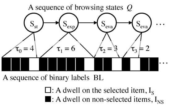
Figure 4.
Segments of browsing states.
The last segment and its length are denoted as [jK–1 + 1, jK] and τK–1 = jK – jK–1, respectively when the last dwell is on the selected item (i.e., jK = J). Meanwhile, when the last dwell is not on the selected item (i.e., jK ≠ J), we consider an additional dwell on the selected item after the last dwell as iJ+1 such that blJ+1 = IS for convenience. This is because the attention of the decision maker is considered to be on the selected item just after the last dwell when the decision maker makes a choice at the end of each decision making session. In this case, the last segment and its length are denoted as [ jK+1, J+1] and τK= (J+1)– jK, respectively.
Besides the first segment, [j1 + 1, j2], we here define the segment until the first dwell on the selected item and its lengths as [1, j1] and τ0 = j1, respectively. The segment before the first dwell on the selected item, [1, j1], should be treated differently to the other segments since the timing of the first dwell on the selected item depends on exogenous factors of content layout rather than browsing states of decision makers. For this, we consider start state in addition to the above mentioned two browsing states. Finally, a sequence of lengths of segments is defined as τ = (τ0, τ1, ..., τKj ), where Kj = K when jK ≠ J, and Kj = K – 1 when jK = J.
Let us denote the two browsing states, the exploration and the evaluation state, as S exp and S eva, respectively, and the start state as S st. Assuming the browsing states do not change during the segments, what we want to estimate here is a sequence of browsing states Q = (q0, q1, ..., qKj ) using the length of each segment as a cue. Note that every decision process starts with the start state in our model (i.e., q0 = S st) and that the states qk ∈ {S exp, S eva}(k = 1, ..., Kj) are to be estimated. In particular, how long it takes until a re-dwell on the selected item occurs in each browsing state (lengths of the segments) in each browsing state is formulated as follows.
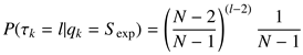
Exploration state. The exploration state is defined to be a state where a decision maker aims to explore information of a whole catalog. Thus, each item in the catalog is considered to be looked at with equal frequency (i.e., a uniform distribution) regardless of whether or not it is the selected item. Assume that the k-th segment is the exploration state and contains the j-th dwell and the (j – 1)-th dwell. Since the (j – 1)-th dwell is not the end of the segment, the (j – 1)-th dwell is on a non-selected item. As mentioned above, the item on the (j – 1)-th dwell and the j-th dwell is always unequal (i j–1 ≠ i j). Thus, when the (j – 1)-th dwell is on a certain item, the j-th dwell can only be on one of the (N – 1) items, where N is the total number of items on the catalog as mentioned above. Accordingly, the probabilities of the j-th dwell being on a nonselected item and on the selected item are represented as P(blj = INS|bl j–1 = INS, qk = S exp) = (N – 2)/(N – 1), and P(blj = IS|bl j–1 = INS, qk = S exp) = 1/(N – 1), respectively.
The probability of the k-th interval lasting l dwells is described as a geometric distribution
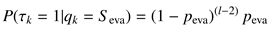
Evaluation state. The evaluation state is defined to be a state where a decision maker aims to obtain more detailed information of a set of specific items (strong candidates). Therefore, in the evaluation state, the probability of a dwell on the selected item is considered to be higher than one in the exploration states. Since we do not know the probability, we introduced a parameter peva to represent the probability of a dwell on the selected item in the evaluation state; that is, P(blj = IS|bl j–1 = INS, qk = S eva) = peva. Thus, the probability of the j-th dwell being on a non-selected item is represented as P(blj = INS|bl j–1 = INS, qk = S eva) = 1 – peva. Here, the value of peva is estimated from eye tracking data in this study. Note that the higher value of estimated peva indicates that the selected item is more likely to be looked at in the evaluation state.
The probability of the k-th interval lasting l dwells is described as a geometric distribution
A hidden Markov based choice behavior model. Since we want to represent free transitions of the browsing states, we employ a hidden Markov model (HMM). The proposed HMM is denoted as λchoice = (S, π, A, L, C). S is a set of browsing states; S = {S st, S exp, S eva}. π is a set of initial state probabilities; π = (πst, πexp, πeva) = (1, 0, 0) since our model assumes decision process always starts from the start state, S st. A is a 3 × 3 state transition probability matrix, where ai, jindicates the transition probability from the i-th state to the j-th state. In our model, ai, jis always set to zero if the j-th state corresponds to the start state, S st. That is, no transition from any states to the start state, S st, occurs including self-transition.
Possible outputs of the model L are lengths of the segments: L = {1, ..., Lmax}, where Lmax is the maximum length of the segments. C is a set of output probabilities. Note the probability of an output l ∈ L in the exploration state and the evaluation state, P(τk= l|qk = S exp) and P(τk= l|qk = S eva), are defined as the Equation (1) and the Equation (2), respectively. The output probabilities in the start state are denoted as {P(τ0 = l)}l. The output probabilities are normalized so that the sum of output probabilities in each state is 1.
Estimation of model parameters and identification of browsing states. The unknown parameters to be estimated here are peva, the probability of dwells on the selected item in the evaluate state, {P(τ0 = l)}l, the output probabilities of the start state, and A, the transition probabilities of hidden states. The output probabilities of the start state are simply calculated as the frequency distribution of the lengths of the first segments of each sequence . The rest of model parameters are estimated by the Baum-Welch algorithm (Baum, Petrie, Soules, & Weiss, 1970). Once the model parameters are estimated, browsing states can be estimated from the sequence of segment lengths, τ, using the Viterbi algorithm.
Evaluation
Our catalog browsing model is evaluated by comparing with previously proposed two decision process models: Russo’s three stage model (R&L) (Russo & Leclerc, 1994) and Natural Decision Segmentation Model (NDSM) (Gidlöf et al., 2013) using the collected gaze data (see the section of Data Collection).
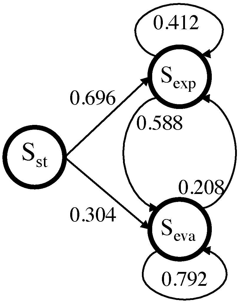
Estimated model parameters. The model parameters are estimated using the eye tracking data of all participants. Figure 5 shows the state transition probabilities. The result shows that the transition from the start state to the exploration state is more likely than one from the start state to the evaluation state. Moreover, the transition from the exploration state to the evaluation state is of higher probability than the opposite transition. This indicates that decision makers tend to start from the exploration state and then gradually shift to the evaluation state.

Figure 5.
The estimated transition probabilities of the browsing states using eye tracking data of all participants.
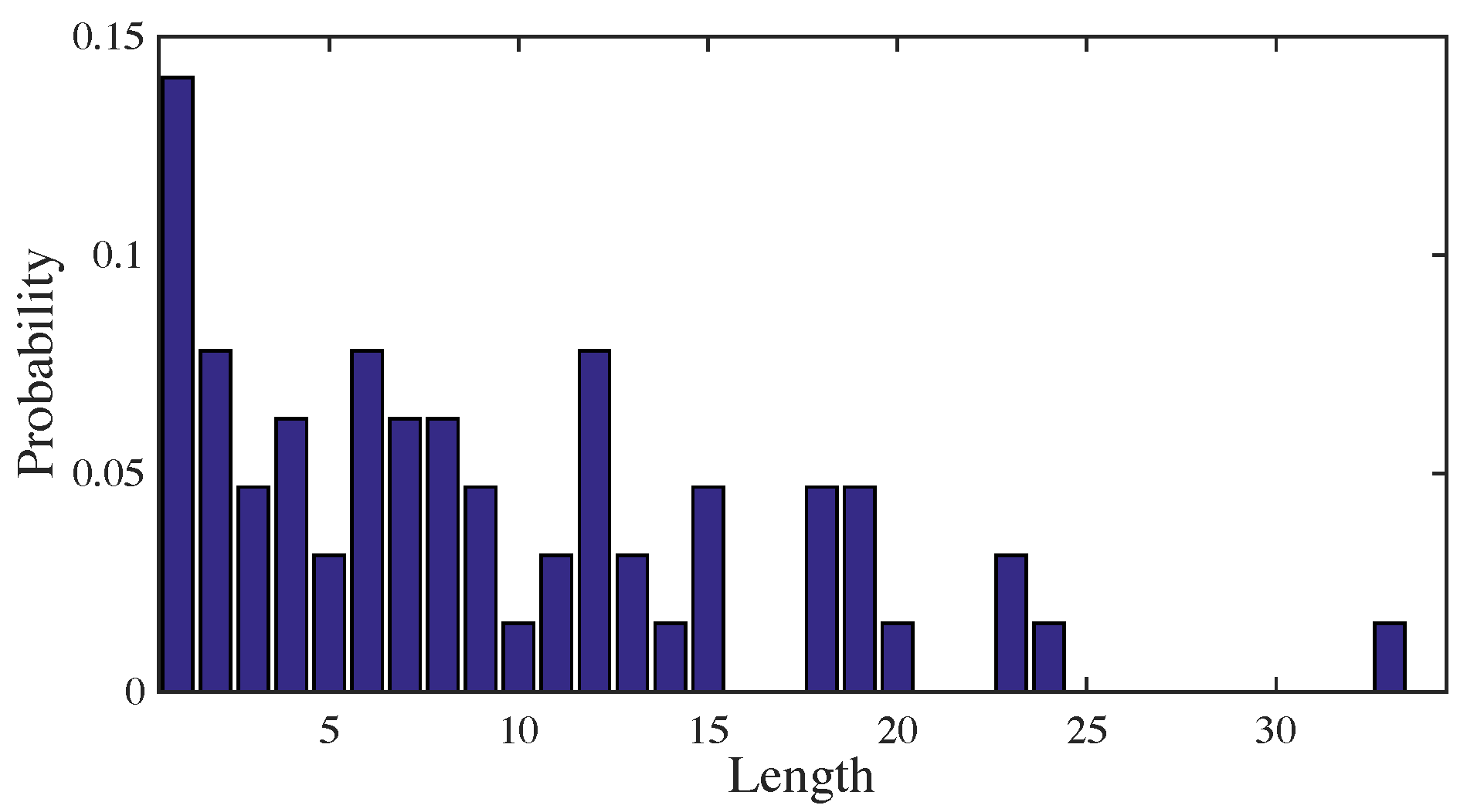
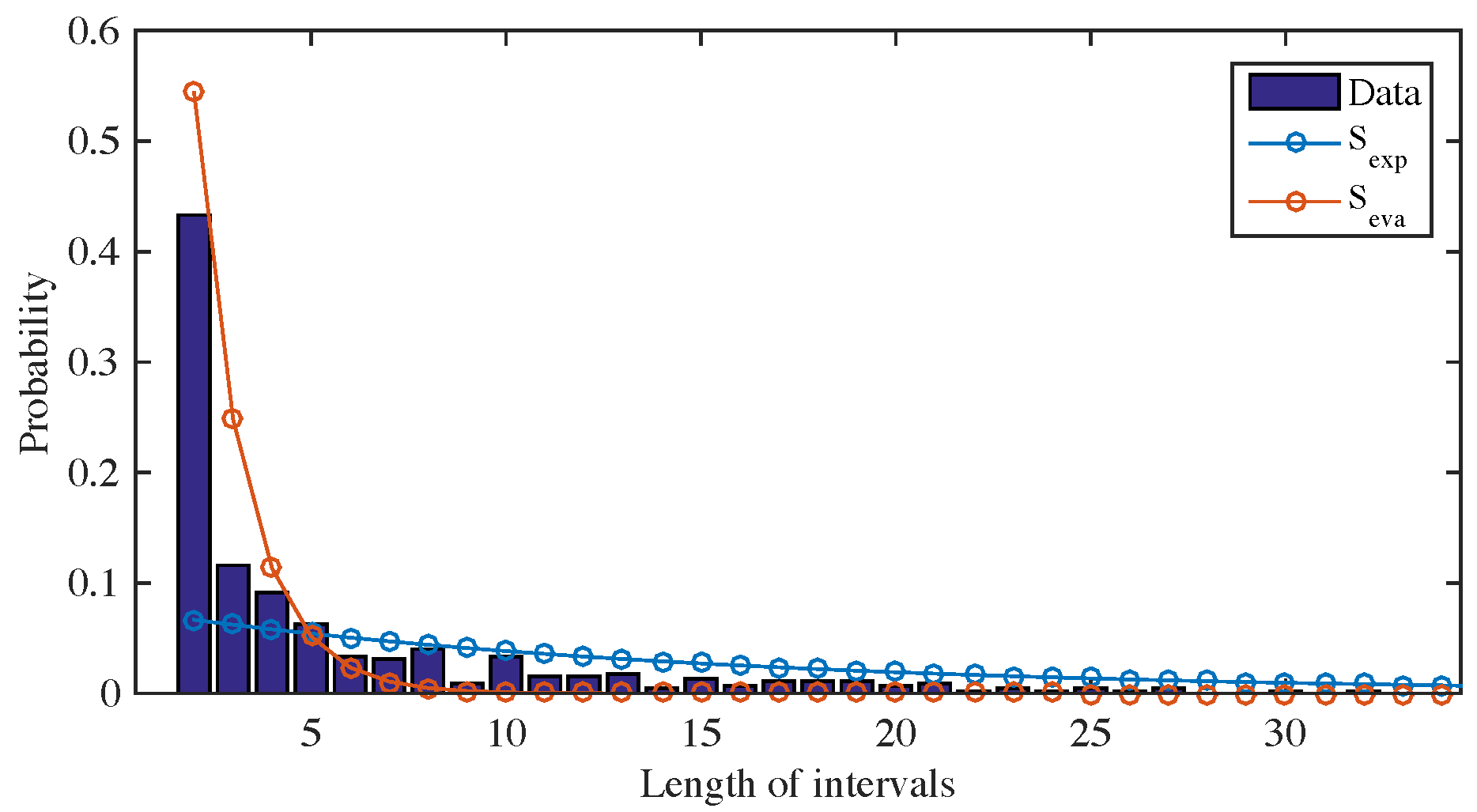
Figure 6 shows the output probabilities of the start state. Figure 7 shows the output probabilities of the exploration/evaluation states and the frequency distribution of lengths of all segments except the first segment (i.e., τ1, ..., τKj ). The frequency distribution in Figure 7 has its peak when the length is 2 (similar to the geometric distribution). The probability of dwells on the selected items in the evaluation state was learned as peva = 0.544. This result shows that decision makers are more likely to look at the selected items within short intervals in the evaluation state.
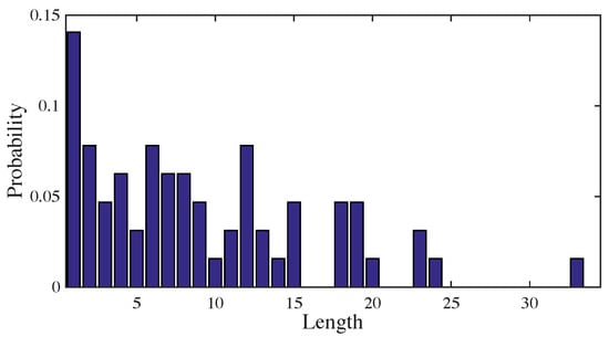
Figure 6.
The output probabilities of the start state, Sst, estimated using eye tracking data of all participants.
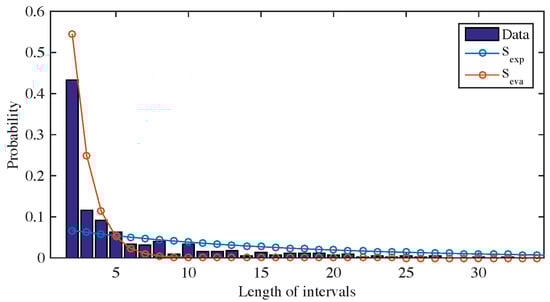
Figure 7.
The output probabilities of the exploration state, Sexp, and the evaluation state, Seva, estimated using eye tracking data of all participants. The bars represent the frequent distribution of segment lengths.
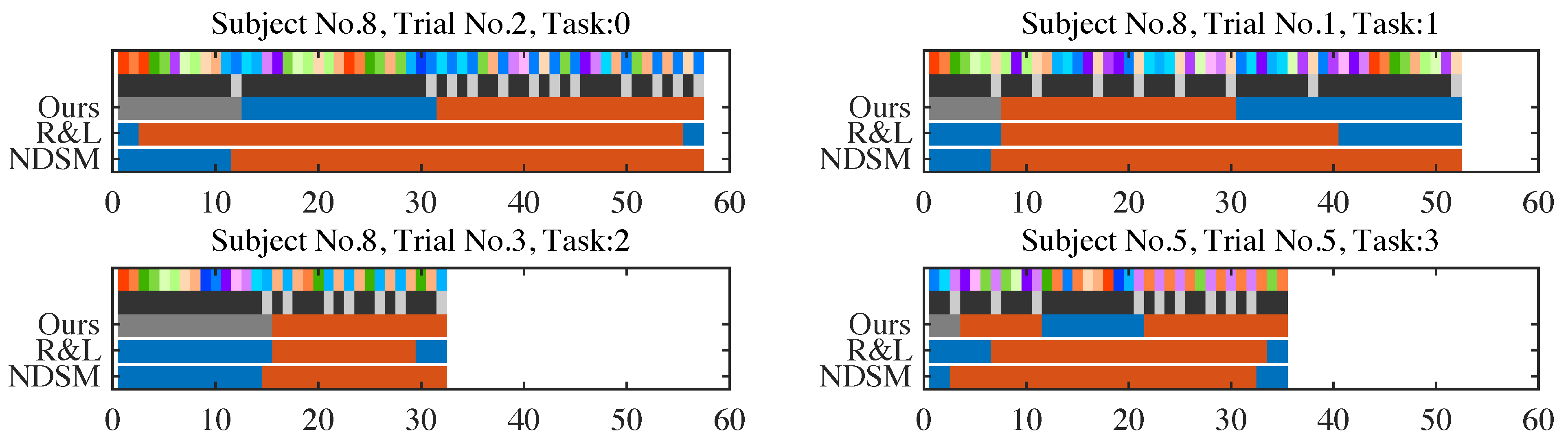
Example sequences of identified states. Four example sequences of identified browsing states by the proposed model and other two comparison models are shown in Figure 8. Only when the selected item was first looked at after the most of items were examined by coincidence, and the first re-dwell pattern occurred at the same time, these three models identify browsing states similarly (see the left bottom example). However, in the most of other cases, participants continue examining other items even after looking at the selected item such as in the left top example. Moreover, in the right bottom example, R&L and NDSM both identify the evaluation state so as to occupy the whole sequence. The gap from the 12th dwell to the 21th dwell where the selected item is less frequently looked at is described only with the proposed method.

Figure 8.
Examples of estimated browsing state sequences. For each sequence, the color in the top row corresponds to the color of regions in Figure 2. In the second row, the timings of the dwells on the selected item is shown by light gray highlights. From the third row to the bottom row, the blue and red intervals correspond to the exploration state and the evaluation state, respectively.
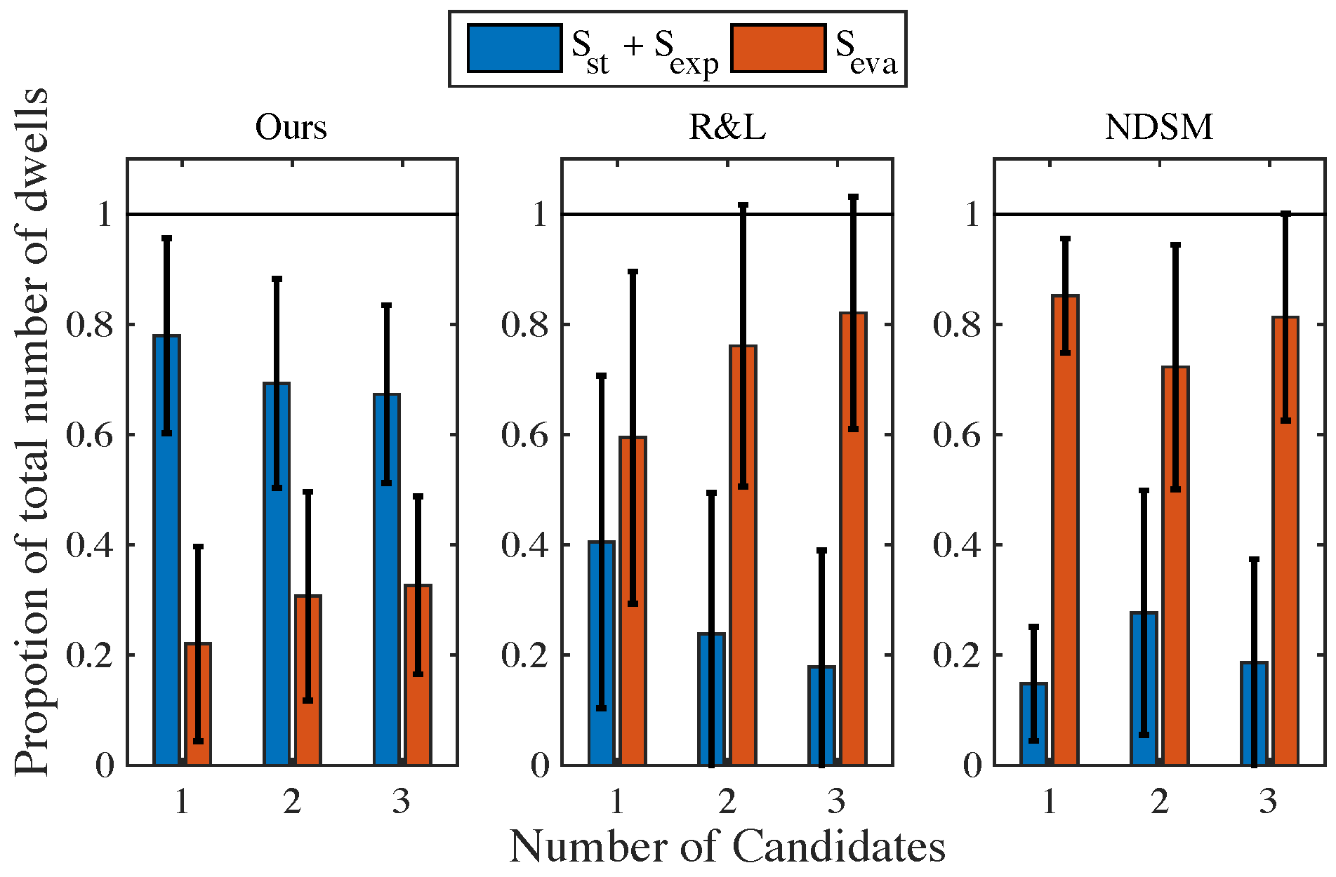
Difficulty of decision tasks and browsing states. Figure 9 shows the mean ratio of the two browsing states with each task type where the number of candidates is 1 to 3. The proposed method and R&L show an increase in the ratio of the evaluation state in tasks with a higher number of strong candidates. There was a significant difference of the ratio of the evaluation state between the task 1 and the task 3 using R&L model (Welch’s t-test; p = .024). Although we did not observe any significant difference for the results of the proposed model and NDSM, the proposed model shows the similar effects of the task to ones with R&L model. These results indicate that our model and R&L can describe differences of browsing behavior between different tasks when compared with NDSM. Note here that we did not consider eye tracking data in tasks where the number of candidates is 0 since the difficulty of the decision task is hard to interpret.
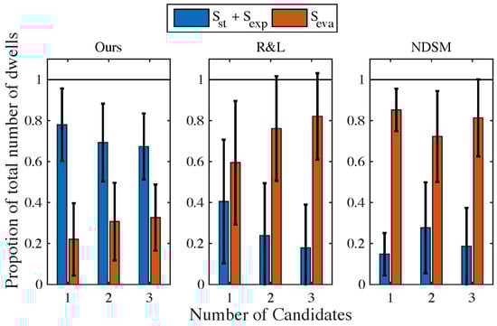
Figure 9.
The proportion of total dwells in browsing states. The whiskers represent standard deviation.
The ratio of the evaluation and exploration states identified using our model is biased towards the exploration state more than the other two comparison models. This indicates that our model is more sensitive to the interruptions of the exploration/evaluation states, which often appear as shown in Figure 8. This result shows that allowing bi-directional transitions of browsing states in the state model is more effective when modeling browsing states.
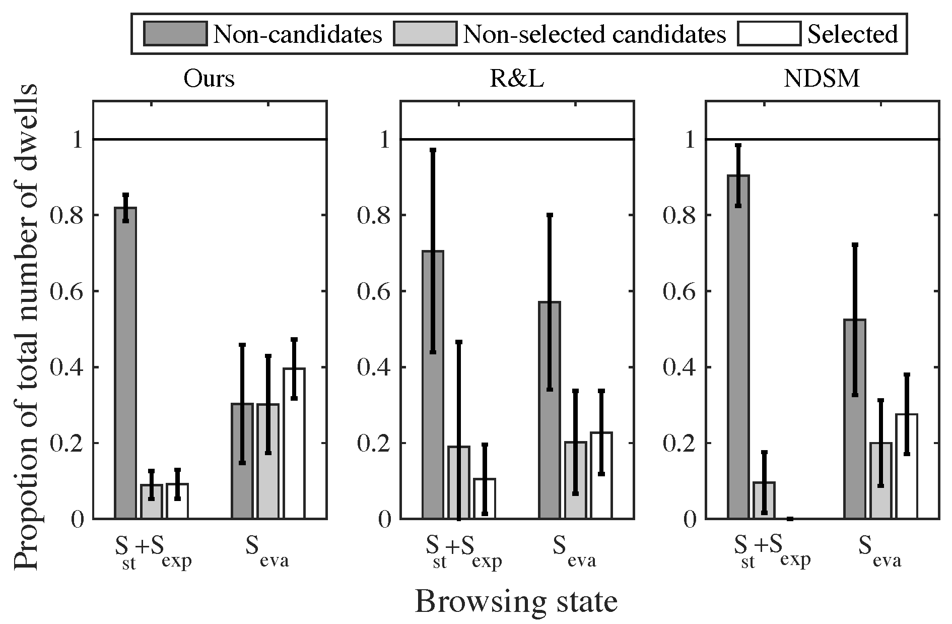
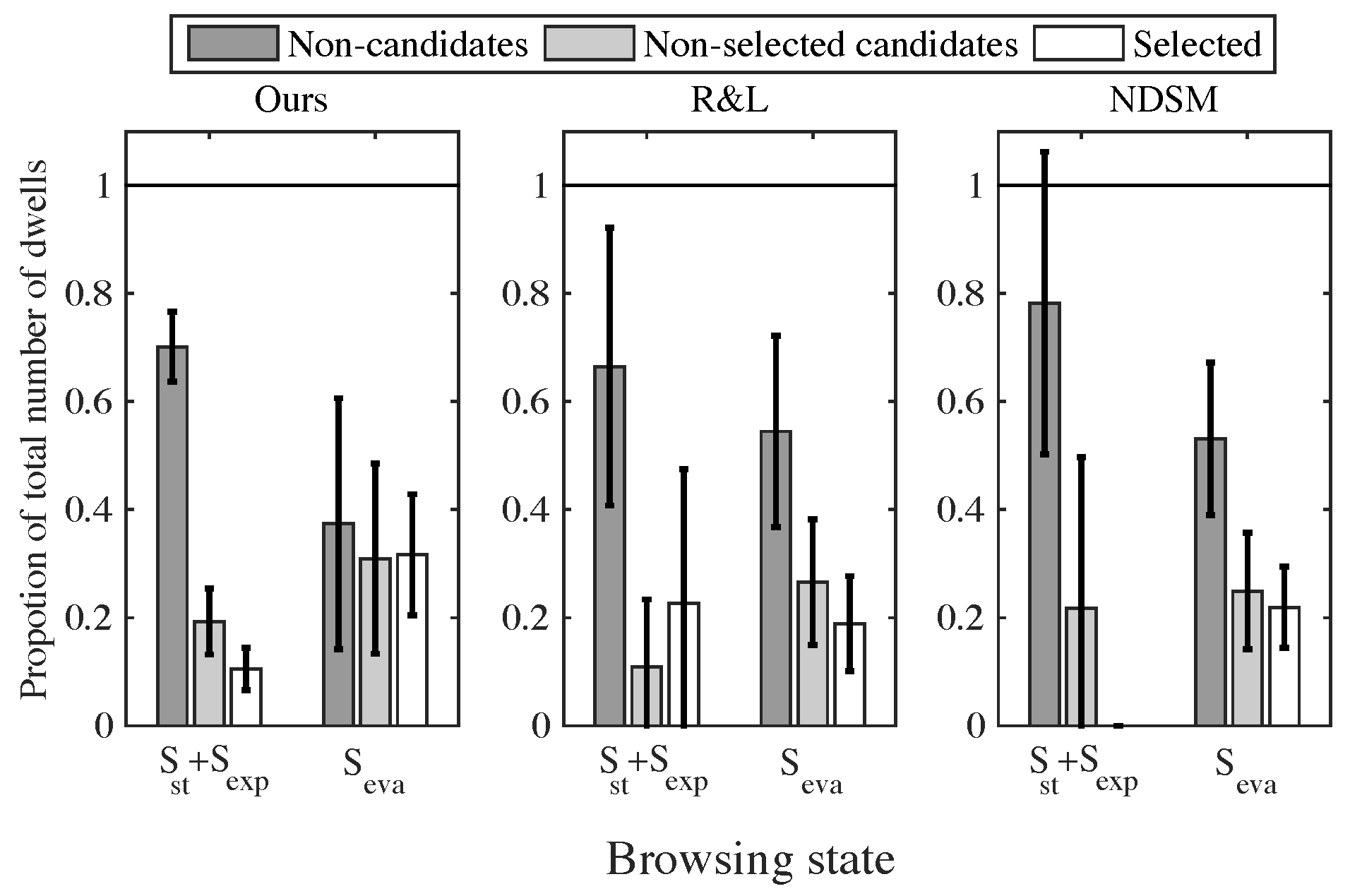
Dwells on non-selected candidates and browsing states. Candidates are the items that satisfy the task (see Data Collection section for the details.). In tasks with more than two candidates, not only how selected items are looked at but also how non-selected candidates are looked at is a good measurement to understand the characteristic of the browsing states. Figure 10 and Figure 11 show the proportion of dwells on each item type: the selected item, non-selected candidates, and the others. Figure 10 shows the results in tasks with two candidates, and Figure 11 shows the results in tasks with three candidates. In the both figures, non-selected candidates are more likely to be looked at in the evaluation states, S eva, compared to the exploration states, S exp. There were significant differences of the ratio of the dwells on non-selected candidates between the exploration state and the evaluation state using our model (Welch’s t-test; p < .001 for twocandidate-tasks and p = .022 for three-candidate-tasks). Using R&L, there was a significant difference between the exploration state and the evaluation state in three-candidatetasks (Welch’s t-test; p = .001). Using NDSM, there was a significant difference between the exploration state and the evaluation state in two-candidate-tasks (Welch’s t-test; p = .009). Only when our model was used, the significant differences were observed in the both tasks.
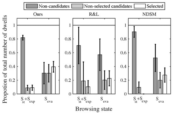
Figure 10.
The proportion of total dwells on selected items, non-selected candidates and the other items when the number of candidates is 2. The whiskers represent standard deviation.
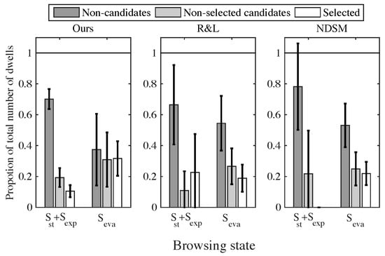
Figure 11.
The proportion of total dwells on selected items, non-selected candidates and other items when the number of candidates is 3. The whiskers represent standard deviation.
Application: Estimation of Browsing States
In this section, we propose an estimation method of browsing states that does not require information of selected items so that it can be used for possible applications such as decision support systems. For example, when an information system can understand browsing states of a user during a decision making task, it enables the system to provide the right information at the right time.
To achieve this, we extend our choice behavior model proposed in the previous section with gaze actions derived by the spatial and semantic structure of the digital catalog on the screen. The following sections first present an overview of the proposed estimation method. Next, the details of how to encode eye movements into gaze actions and how our choice behavior model is associated with the gaze actions is presented.
The overview of our estimation method
Suppose we have a set of dwell sequences 5 = {Iu = (i1, ..., iJu )}uand corresponding sequences of browsing states Q = {Qu = (q1, ..., qJu )}uas training data, where u is the id of recorded eye tracking sequences. Q is obtained by our choice behavior model, λchoice. In this situation, the goal is to estimate browsing states from a newly observed gaze data without the information of the selected item.
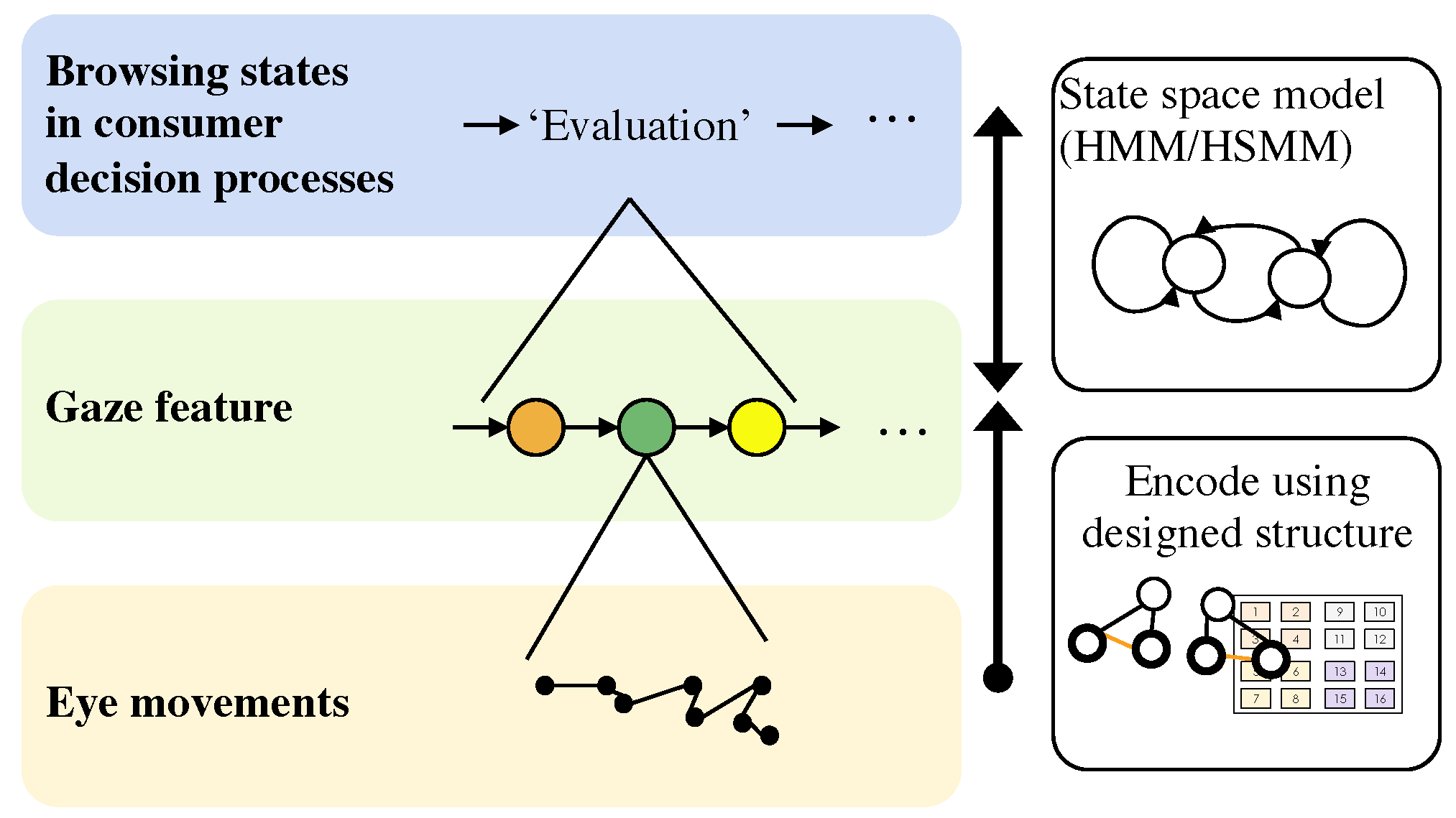
The overview of the proposed estimation method is shown in Figure 12. Eye movements are first encoded to a sequence of gaze features using a semantic structure of the catalog, called designed structure (Ishikawa, Kawashima, & Matsuyama, 2015). Designed structure is high-level content structure that reflects the designer’s point of view such as groupings of items. Instead of using semantic attributes of items, the designed structure employs embedded semantic information as a content layout. This has an advantage on dealing with the above mentioned decision-support situations since it can be applied to any visual contents as long as they share the same layout. Second, the probabilistic relations between the gaze features and browsing states are learned. Once the model is learned, we can estimate browsing states of newly observed eye tracking data using the learned model.
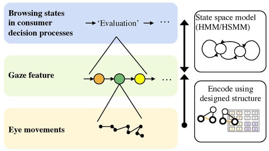
Figure 12.
Overview of the estimation method.
Gaze features
Modeling of content structure. The designed structure can be represented as follows. As with the previous section, suppose a catalog contains information of a set of items 5All = {1, ..., N}. Each item has a set of P attributes PAll = {1, ..., P}, where p-th attribute can take a value of Ap possible attribute values A(p) = {1, ..., Ap}. Here, let us introduce a function fp : 5All → A(p), where fp(i) indicates the attribute value of the p-th attribute that the i-th item has. In the content layout used in the experiment, the designer aims to emphasize a specific attribute (e.g., category), then all items in the same category are regarded as “in the same group” and allocated based on their category type. To represent this process, a set of the emphasized attributes is described as PE ⊂ PAll. Using PE, the relations among items in the digital catalogs can be determined as follows.
Parallel relation. Two different items i and j have this relation when the items share one or more emphasized attributes; that is, fp(i) = fp(j), ∃p ∈ PE.
Contrast relation. Two different items i and j have this relation when the items do not share any emphasized attributes; that is, fp(i) ≠ fp(j), ∀p ∈ PE.
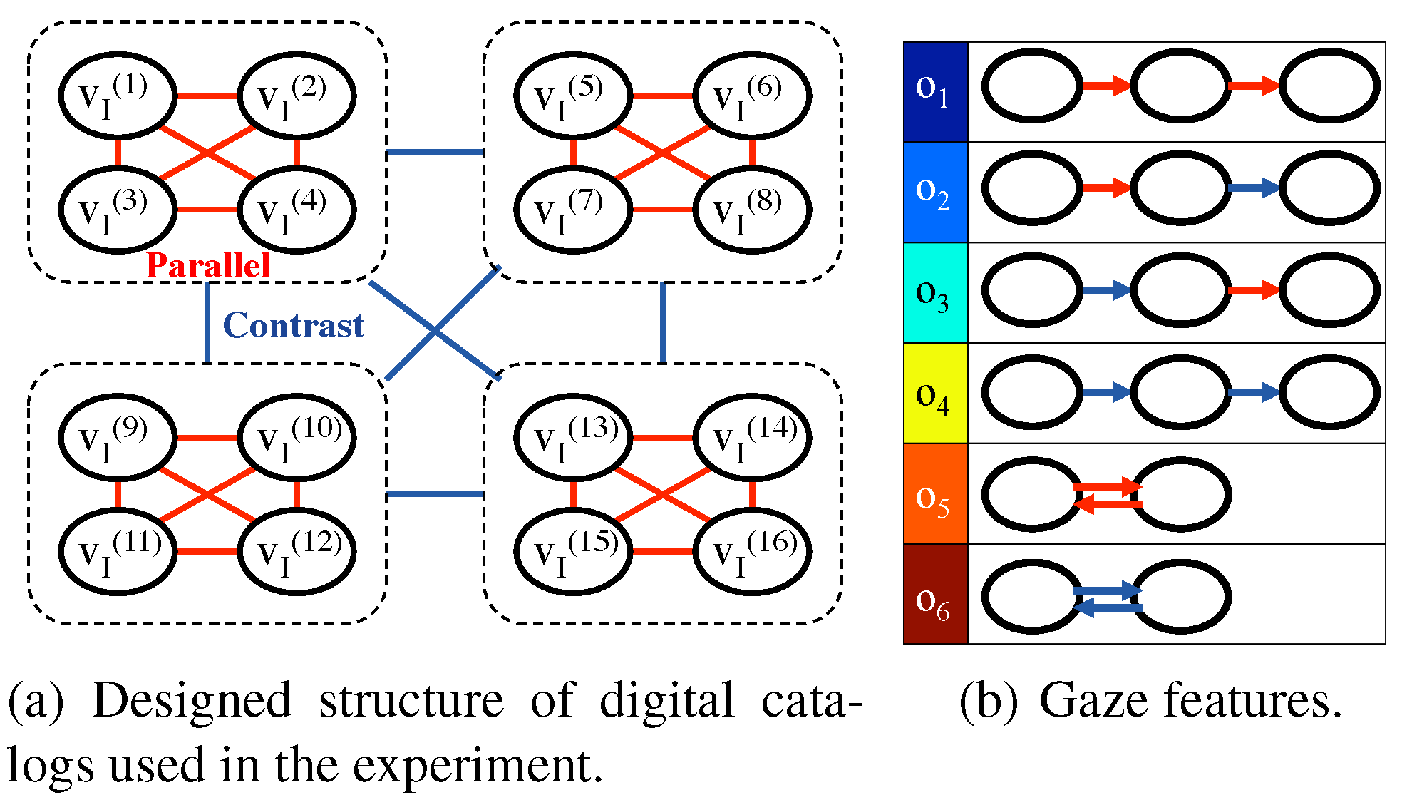
The versatility of the use of designed structure is confirmed by using multiple types of layouts (Ishikawa et al., 2015). This paper focuses on analysis of the sequence of encoded gaze features. Therefore, we only use catalogs with categorybased layout that can be simply described by the above two relations. We represent the relations among items as a directed graph for the encoding of eye movements. Let us denote a set of nodes VI = {v(n) | n = 1, ..., N} corresponding to the K items. Here, design-relation edges are defined as ED ⊆ VI × VI, where each edge ed ∈ ED has either label parallel or contrast. Finally, the designed structure is defined by a directed graph GD = (VI, ED) (as shown in Figure 13 (a)).

Figure 13.
Encoding of eye movements. (a) Edges between dotted frames indicate that every node in the frame is connected to every node in the other frame. (b) Six patterns of tri-gram paths in the graph GD. The two bottom features correspond to comparison patterns in which the first and the last dwell of the tri-gram is on the same item.
Encoding eye movements into gaze features. A sequence of dwells on items, I = (i1, ..., iJ) i j ≠ i j+1, i j ∈ 5All , is associated with design relation labels derived from the graph of the designed structure, GD. For simplicity, the id of eye tracking sequences, u, is omitted in this section. For each tri-gram of gaze regions (i j–1, i j, i j+1) (j ∈ {2, ..., J – 1}) in a gaze region sequence, a path of corresponding item nodes in the graph GD is obtained. Tri-gram patterns of gaze regions is a gaze feature often used in previous eye tracking studies (Nakano & Ishii, 2010; Bulling, Ward, Gellersen, & Troster, 2011; Kübler, Kasneci, & Rosenstiel, 2014). By considering only the labels of edges of each path, we can categorize the paths into six patterns {o1, ..., o6} as shown in Figure 13 (b). Note that the four top features in Figure 13 (b) correspond to tri-grams with three different gaze regions, that is, i j–1 ≠ i j+1, and the two bottom ones correspond to binary comparison patterns in which the first and the last dwell of the tri-gram is on the same item (i j–1 = i j+1). Finally, a sequence of gaze features is obtained as X = (x2, ..., xJ–1), (xj ∈ {o1, ..., o6}).
Modeling probabilistic relations of gaze features and browsing states
Our choice behavior model is denoted as λchoice = (S, π, A, L, C) (see the section of Proposed model for the details). We modify the model, λchoice, to a hidden semi-Markov model (HSMM) λHSMM to associate the gaze actions with the browsing states.
HSMM (also known as explicit duration hidden Markov model) is an extension of HMM that considers additional parameters for explicitly modeling the duration of states. The most important difference between λchoice and λHSMM is that the outputs of λHSMM are the gaze features, meanwhile, the outputs of λchoice are the interval lengths between dwells on the selected item.
The proposed HSMM is denoted as λHSMM = (SHSMM, OHSMM, AHSMM, BHSMM, PHSMM, πHSMM). A set of hidden states SHSMM, initial state probabilities πHS MM, and state transition probabilities AHSMM are common to the choice behavior model, λchoice, that is, SHSMM = S = {S st, S exp, S eva}, AHSMM = A, and πHS MM= π = (πst, πexp, πeva) = (1, 0, 0). OHSMM is a set of gaze feature labels; OHSMM = {o1, ..., o6} (see Figure 13 (b)). BHSMM is a 3 × 6 output probability matrix, where bi,m indicates the output probability of the m-th gaze feature at the i-th browsing state. PHSMM is a 3×Tmax duration distribution matrix, where pi,l indicates the probability that the i-th state last for l-time units.
The duration distribution matrix, PHSMM, represent interval lengths between dwells on the selected item in the choice model, λchoice. That is, pi,l = ci(l), where ci(l) indicates the probability of the segment of length l at the i-th state in the choice model (see the section of A hidden Markov based choice behavior model for the details). Assuming the training gaze dataset: a set of gaze feature sequences, X = {Xu = (x2, ..., xJu –1)}u, and corresponding browsing state sequences, Q, obtained using the choice model, λchoice, the unknown output probabilities, BHSMM, are simply estimated as follows:
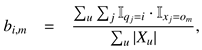
where IAis an indicator function that has the value 1 when A is true and the value 0 otherwise. Once the parameters are obtained, the browsing states of a newly observed gaze data can be estimated by maximum a posterior estimation.
Evaluation
The proposed estimation method is evaluated on the data described in section Data Collection. The output probabilities of the HSMM estimated by the Equation (3) with gaze data from all participants are shown in Figure 14. The results show that the output probabilities of the start state and ones of the exploration state are more similar compared to ones of the evaluation state. In the evaluation state, the gaze feature that consists of contrast relations (o4) and comparison patterns (o5 and o6) occur more frequently than in the start state and the exploration state. This indicates that decision makers tend to browse catalogs more freely by ignoring groups of items in the evaluation state.
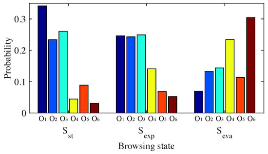
Figure 14.
The output probabilities of each browsing state. The color of the bars corresponds to the color of gaze features in Figure 13 (b).
Consistency with the identified browsing states. Subject based leave-one-out cross validation was used; that is, gaze data of one participant was used as test data and the remaining of the data was used to train the model. We compare our proposed method (HSMM) against two methods: hidden Markov model based estimation (HMM) and maximum likelihood estimation (ML). In the HMM method, a three state HMM (SHMM, OHMM, AHMM, BHMM, πHMM), where SHMM = S, OHMM = O, πHMM = π is trained with the training gaze data: a set of gaze feature sequences, X, and corresponding browsing state sequences, Q. Then, the browsing states can be estimated using the trained HMM by Viterbi algorithm. In the ML method, the browsing state at a timing j, qj, is simply estimated by comparing the likelihood of the observed gaze feature, x j, using the output probabilities of the HSMM based model, λrmHS MM. That is, qj = maxi P(xj = om|q j =i) = bi,m.
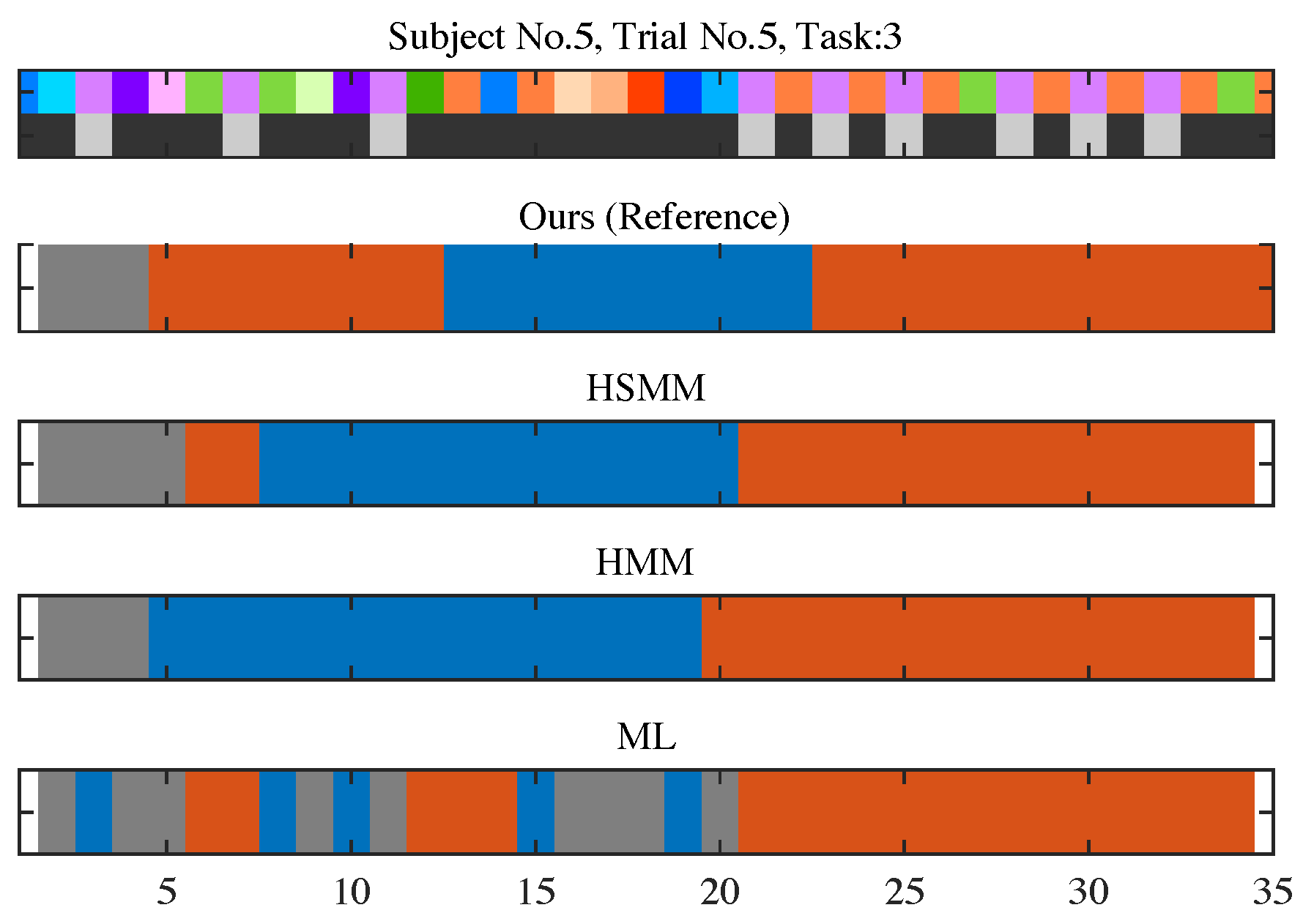
The validity of the estimated browsing states is measured by the consistency to the browsing states of the proposed choice model (the “ground truth” of browsing states). Table 3 shows the consistency of each method. The result shows that the proposed HSMM method has the highest consistency with the ground truth. Example sequences of estimated browsing states are shown in Figure 15. We can see that the HSMM method replicates the ground truth of browsing states better than other methods; the HMM method missed the first evaluation state, and the ML method cannot discriminate the start state and the exploration state.
Table 3.
The consistency with the ground truth. The top row indicates the consistency when we consider that the exploration state Sexp and the start state S st are the same state. The bottom row indicates the consistency when we discriminate the two states.
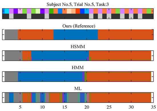
Figure 15.
Example sequences of estimated browsing states. The blue and red intervals correspond to the exploration state and the evaluation state, respectively. The gray interval corresponds to the start state.
Discussion
The gaze data we collected in this study have shown the variety of consumer decision process. We observed various cases of decision process in terms of browsing states. For example, some decision makers change browsing states frequently; meanwhile, others just shift their state from the start/exploration state to the evaluation state. The observations show that the probabilistic approach of modeling browsing behavior in consumer decision process is effective in terms of detecting comparison behavior in the evaluation states compared to a top-down rule based approach.
In this paper, we investigated the relation between complexity of decision tasks (the number of strong candidates) and transitions of browsing states of decision maker. The results of this study indicate that more complex the task gets, the greater the ratio of the evaluation state gets. In this paper, we only built a single model using all collected gaze data; however, the difference between tasks we observed might indicate the necessity of multiple models that correspond to different decision tasks. Moreover, it is also possible that the personality of decision makers and the decision strategy affect the transitions of browsing states. To improve the choice model, we need to collect and analyze more gaze data in different decision situations.
Possible extensions of the proposed choice model. The proposed choice behavior model in this paper consists of the minimum number of hidden states that can represent our assumptions: two browsing states (exploration and evaluation) and a start state. This is because we aimed to keep our model as simple as possible in order to avoid overfitting since the amount of data was limited. However, we yet do not know how many states are most appropriate to represent browsing states in choice behavior. For example, we might need to discriminate the first exploration state and interruptions of exploration states that appear later in a session. In that case, we can consider to optimize the number of states in a data-driven manner by maximizing the likelihood of the model.
Moreover, gaze behavior of decision makers is expected to be affected by exogenous factors at the beginning of decision process. For example, in our situation where a decision maker is browsing a digital catalog, the decision maker tends to confirm all alternatives before proceeding to their detailed evaluation. The choice model might have to be extended so that it can manage the effects of the exogenous factor such as the number of alternatives or layouts of catalogs.
Other gaze features to identify browsing states. We used how often the selected item is looked at to identify browsing states. However, there are some other cues derived from eye movements that might be useful as well such as fixation duration. To find appropriate gaze features for decision stage analysis, it would be possible to apply a statistical approach of feature selection using a huge gaze dataset.
Conclusion
This paper proposed a probabilistic gaze model to understand browsing states in a multi-alternative choice situation. The proposed model is based on a couple of simple assumptions about how often the selected item is looked at to identify browsing states and the rest of the model is estimated in a bottom-up manner. This approach enables the representation of complex choice behavior including interruptions of browsing states. We confirmed the validity of the proposed model through an eye tracking experiment in a catalog browsing situation. The results showed that our model can identify when a participant is exhibiting comparison behavior among candidate items better than comparison models. We also proposed an estimation method of browsing states that does not require the information of the selected item for applications such as interactive information systems.
Acknowledgments
This work is supported by JSPS KAKENHI Grant Numbers 13J05396, 26280075 and JST, PRESTO.
References
- Baum, L. E.; Petrie, T.; Soules, G.; Weiss, N. A maximization technique occurring in the statistical analysis of probabilistic functions of markov chains. The Annals of Mathematical Statistics 1970, 41(1), 164–171. Available online: http://projecteuclid.org/euclid.aoms/1177697196. [CrossRef]
- Bulling, A.; Ward, J. A.; Gellersen, H.; Troster, G. Eye movement analysis for activity recognition using electrooculography. IEEE Trans. on Pattern Analysis and Machine Intelligence 2011, 33(4), 741–753. Available online: http://ieeexplore.ieee.org/document/5444879/. [CrossRef] [PubMed]
- Clement, J. Visual influence on in-store buying decisions: An eye-track experiment on the visual influence of packaging design. Journal of Marketing Management 2007, 23(9-10), 917–928. Available online: http://www.tandfonline.com/doi/abs/10.1362/026725707X250395. [CrossRef]
- Gidlöf, K.; Wallin, A.; Dewhurst, R.; Holmqvist, K. Using eye tracking to trace a cognitive process: Gaze behaviour during decision making in a natural environment. Eye Movement Research 2013, 6(1), 1–14. Available online: http://www.jemr.org/online/6/1/3. [CrossRef]
- Glaholt, M. G.; Reingold, E. M. Eye movement monitoring as a process tracing methodology in decision making research. Journal of Neuroscience, Psychology, and Economics 2011, 4(2), 125–146. Available online: http://psycnet.apa.org/journals/npe/4/2/125/. [CrossRef]
- Glöckner, A.; Herbold, A.-K. An eyetracking strudy on information processing in risky decisions: Evidence for compensatory strategies based on automatic processes. Journal of Behavioral Decision Making 2011, 24(1), 71–98. Available online: http://onlinelibrary.wiley.com/doi/10.1002/bdm.684/abstract. [CrossRef]
- Groner, R.; Groner, M. Groner, R., Fraisse, P., Eds.; Towards a hypothetico-deductive theory of cognitive activity. In Cognition and eye movements; North Holland; Amsterdam, 1982; pp. 100–121. [Google Scholar]
- Groner, R.; Groner, M. Groner, R., Menz, C., Fisher, D., Monty, R., Eds.; A stochastic hypothesis testing model for multi-term series problems, based on eye fixations. In Eye movements and psychological functions: International views; Lawrence Erlbaum, 1983; pp. 257–274. [Google Scholar]
- Groner, R.; Spada, H. Spada, H., Kempf, W., Eds.; Some markovian models for structural learning. In Structural models of thinking and learning; Huber, 1977; pp. 131–159. [Google Scholar]
- Ishikawa, E.; Kawashima, H.; Matsuyama, T. Using designed structure of visual content to understand content-browsing behavior. IEICE Transactions on Information and Systems 2015, 98(8). Available online: http://repository.kulib.kyoto-u.ac.jp/dspace/bitstream/2433/202911/1/transinf.2014EDP7422.pdf. [CrossRef]
- Kübler, T. C.; Kasneci, E.; Rosenstiel, W. Subsmatch: Scanpath similarity in dynamic scenes based on subsequence frequencies. Proceedings of the Symposium on Eye Tracking Research and Applications 2014, 14, 1–5. Available online: http://dl.acm.org/citation.cfm?id=2578206&dl=ACM&coll=DL&CFID=691207058&CFTOKEN=21972424. [CrossRef]
- Liechty, J.; Pieters, R.; Wedel, M. Global and local covert visual attention: Evidence from a bayesian hidden markov model. Psychometrika 2003, 68(4), 519–541. Available online: http://link.springer.com/article/10.1007%2FBF02295608. [CrossRef]
- Nakano, Y.; Ishii, R. Estimating user’s engagement from eye-gaze behaviors in human-agent conversations. In The 15th international conference on intelligent user interfaces; 2010; pp. 139–148. Available online: http://dl.acm.org/citation.cfm?id=1719990. [CrossRef]
- Orquin, J. L.; Loose, S. M. Attention and choice: A review on eye movements in decision making. Acta psychologica 2013, 144(1), 190–206. Available online: http://www.sciencedirect.com/science/article/pii/S0001691813001364. [CrossRef]
- Payne, J. W. Task complexity and contingent processing in decision making: An information search and protocol analysis. Organizational Behavior and Human Performance 1976, 16(2), 366–387. Available online: http://www.sciencedirect.com/science/article/pii/0030507376900222. [CrossRef]
- Payne, J. W.; Bettman, J. R.; Johnson, E. J. The adaptive decision maker; Cambridge: Cambridge University Press, 1993; Available online: http://www.cambridge.org/us/academic/subjects/psychology/cognition/adaptive-decision-maker?format=PB&isbn=9780521425261.
- Pfeiffer, J.; Meißner, M.; Prosiegel, J.; Pfeiffer, T. Classification of goal-directed search and exploratory search using mobile eye-tracking. In The 5th international conference on information systems; 2014; pp. 1–14. Available online: http://aisel.aisnet.org/icis2014/proceedings/GeneralIS/21/.
- Pieters, R.; Warlop, L. Visual attention during brand choice: The impact of time pressure and task motivation. Research in Marketing 1999, 16(1), 1–16. Available online: http://www.sciencedirect.com/science/article/pii/S0167811698000226. [CrossRef]
- Reutskaja, E.; Nagel, R.; Camerer, C. F.; Rangel, A. Search dynamics in consumer choice under time pressure: An eye-tracking study. The American Economic Review 2011, 101(2), 900–926. Available online: https://www.aeaweb.org/articles?id=10.1257/aer.101.2.900. [CrossRef]
- Russo, J.; Leclerc, F. An eye-fixation analysis of choice processes for consumer nondurables. Consumer Research 1994, 21(2), 274–290. Available online: http://www.jstor.org/stable/2489820. [CrossRef]
- Russo, J.; Rosen, L. An eye fixation analysis of multialternative choice. Memomry & Cognition 1975, 3(3), 267–276. Available online: http://link.springer.com/article/10.3758/BF03212910. [CrossRef]
- Shi, S. W.; Wedel, M.; Pieters, F. R. Information acquisition during online decision making: A model-based exploration using eye-tracking data. Management Science 2013, 59(5), 1009–1026. [Google Scholar] [CrossRef]
- Shimojo, S.; Simion, C.; Shimojo, E.; Scheier, C. Gaze bias both reflects and influences preference. Nature Neuroscience 2003, 6(12), 1317–1322. Available online: http://www.nature.com/neuro/journal/v6/n12/full/nn1150.html. [CrossRef]
- Simola, J.; Salojärvi, J.; Kojo, I. Using hidden markov model to uncover processing states from eye movements in information search tasks. Cognitive Systems Research 2008, 9(4), 237–251. Available online: http://www.sciencedirect.com/science/article/pii/S1389041708000132. [CrossRef]
- Stüttgen, P.; Boatwright, P.; Monroe, R. T. A satisficing choice model. Marketing Schience 2012, 31(6), 878–899. [Google Scholar] [CrossRef]
- Sugano, Y.; Ozaki, Y.; Kasai, H.; Ogaki, K. Image preference estimation with a data-driven approach: A comparative study between gaze and image features. Eye Movement Research 2014, 7(3), 1–9. Available online: http://www.jemr.org/online/7/3/5. [CrossRef]
- Wedell, D. H.; Senter, S. M. Looking and weighting in judgment and choice. Organizational Behavior and Human Decision Processes 1997, 70(1), 41–64. Available online: http://www.sciencedirect.com/science/article/pii/S0749597897926923. [CrossRef] [PubMed]
- Yu, S.-Z. Hidden semi-markov models. Artificial Intelligence 2010, 174(2), 215–243. Available online: http://linkinghub.elsevier.com/retrieve/pii/S0004370209001416. [CrossRef]


Copyright © 2024. This article is licensed under a Creative Commons Attribution 4.0 International License.