Evidence for a Structural Analysis of Target Selection in Picture Viewing

Abstract

Spontaneous fixations onto shapes are driven by a structural analysis. But is such analysis also carried out during free viewing of real-world scenes? Here, we analyze how fixation locations in such scenes are related to their region using the region's symmetric axes as a reference. Each fixation location is compared with respect to its nearest symmetric-axis segment by a latitude and a longitude measure. Analyzing the distributions for the two measures we find that there exist fixation biases for L features and parallel contours, suggesting that structural analysis may play a role in saccadic target selection during free viewing.

1. Introduction

There exist two principal approaches to the study of spontaneous saccadic target selection. One approach has studied where exactly saccades land on simple shapes or structures (e.g. Richard and Kaufmann, 1969; Melcher and Kowler 1999) and it has yielded insight into the possible mechanisms of shape analysis for target selection. Experiments of this approach tend to present isolated shapes, that is without being embedded in the context of a visual scene. The other approach has focused on an analysis of fixation locations, which were made during freeviewing of pictures (complex scenes). A common methodof this approachis to characterize target selection in terms of the statistical or simple-feature composition of locations selected for fixation (e.g. Reinagel and Zador 1999; Itti and Koch 2001; Tatler et al, 2005). In its purest form, this approach ignores higher-level structures such as shape in scenes. However, it has become increasingly clear that structural components such as objects (Einhäuser et al., 2008), scene gist (Torralba et al., 2006), and scene segmentation process (Zelinsky & Schmidt, 2009) all have fundamental influences on target selection in images of natural scenes. To date, there has been no effort to combine the two approaches, namely to extend the findings of the former (isolated-shape) approach to the analysis of fixations made in pictures. In this study we attempt a first step into that direction. In common with the majority of contemporary investigations of the locations chosen for fixation, we do not consider the sequence in which these locations are selected. Sequential understanding of selecting is of course important, and has formed the basis of a considerable body of research dealing with scan-path analysis (e.g., Noton & Stark, 1971; Groner et al., 1984; Menz & Groner, 1985; Locher et al., 1993). However, the focus in our work lies in particular on the structure, that was selected by a single fixation, irrespective of when that fixation occurred.

Richard and Kaufmann found that when subjects are asked to move their fovea on a simple shape, that they place their gaze at varying but preferred locations: for closed shapes (triangle, circle, rectangle) saccades land in or around their center; for intersecting lines (crosshair, gap between two collinear straight segments) they land directly on the intersection; for a rectangular L feature they land toward the corner. Kaufman and Richard (1969) explain these observations by proposing that those preferred locations can be associated with the symmetric axes obtained from Blum’s symmetric-axis transform (1967). Melcher and Kowler analyzed this target selection in much more detail. They explored three possible structural key points that might act as saccade targets: the center-of-gravity (COG), the center-of-area (COA) and the symmetric axis. For a given shape, the COG was taken as the average location of all contour pixels, the COA as the center-of-mass of the shape when it is filled with points of uniform density. Subjects were instructed to move their eyes from a fixation cross to the shape without particular time constraints. The shape extended ca. 2 degrees and was around 4 degrees eccentric (from the crosshair). Under these rigid conditions, a subject’s fovea lands closest to the COA. The fact that in these studies a close association between fixation location and key points was found, suggests that these structural features have a role to play in the decision about where to fixate. Thus, it would appear that for isolated shapes, saccadic target selection relies at least in part on a structural analysis.

But does this structural analysis also occur when complex scenes are viewed? The line-drawing studies by Noton and Stark (1971) provide some initial evidence that this may be so. Originally, the authors sought evidence for the presence of a fixed, temporal order in fixation locations. Even though this seems not to be the case in this strong form, the data clearly show that subjects tended to fixate intersecting contours as well as regions: for instance for the nonsense shape (left column of their Figure on page 42) some fixations landed near the intersection of the joint between a straight segment and a circle, and this was found for several subjects; for the right column (head with hand at chin), subjects tended to fixate the pattern depicting the fingers of the hand. From this study it is possible to suggest that in the more complex situation of a line drawing containing multiple key points, structural analysis may again play a role in saccade target selection. Interestingly in this context participants had multiple possible targets for fixation rather than isolated shapes as in the previous examples. However, the line drawings used by Noton and Stark are still some way from what we would refer to as a natural scene.

Images of natural scenes have added complexity in a number of ways. For example, objects are embedded with the context of textured backgrounds rather than in isolation. Furthermore, the structural key points that are associated with objects and scene regions can occur at multiple spatial scales. Thus teasing apart the scales that contribute to target selection is far from trivial. Just by looking at the fixation locations in Figure 2, one can observe that subjects sometimes look into regions in which structural analysis could be at several different scales, such as the fixations on the brick wall. Here the bricks are only available for structural analysis at the finest spatial scales, but the larger region of this section of wall may guide fixation placement at a much coarser scale, at which the individual bricks are no longer resolvable. Because multiple scales may be involved in fixation placement, it is important to consider a set of spatial scales in the fixation analysis.

In the present paper, we look for any evidence that structural analysis might play a role in saccade targeting when freely viewing images of natural scenes. We follow the logic employed for simple shapes that if fixations are placed systematically with respect to a key point, then we can infer that this key point may be in some way involved in saccade target selection. We therefore look for any correlation between fixation placement and key points in complex scenes.

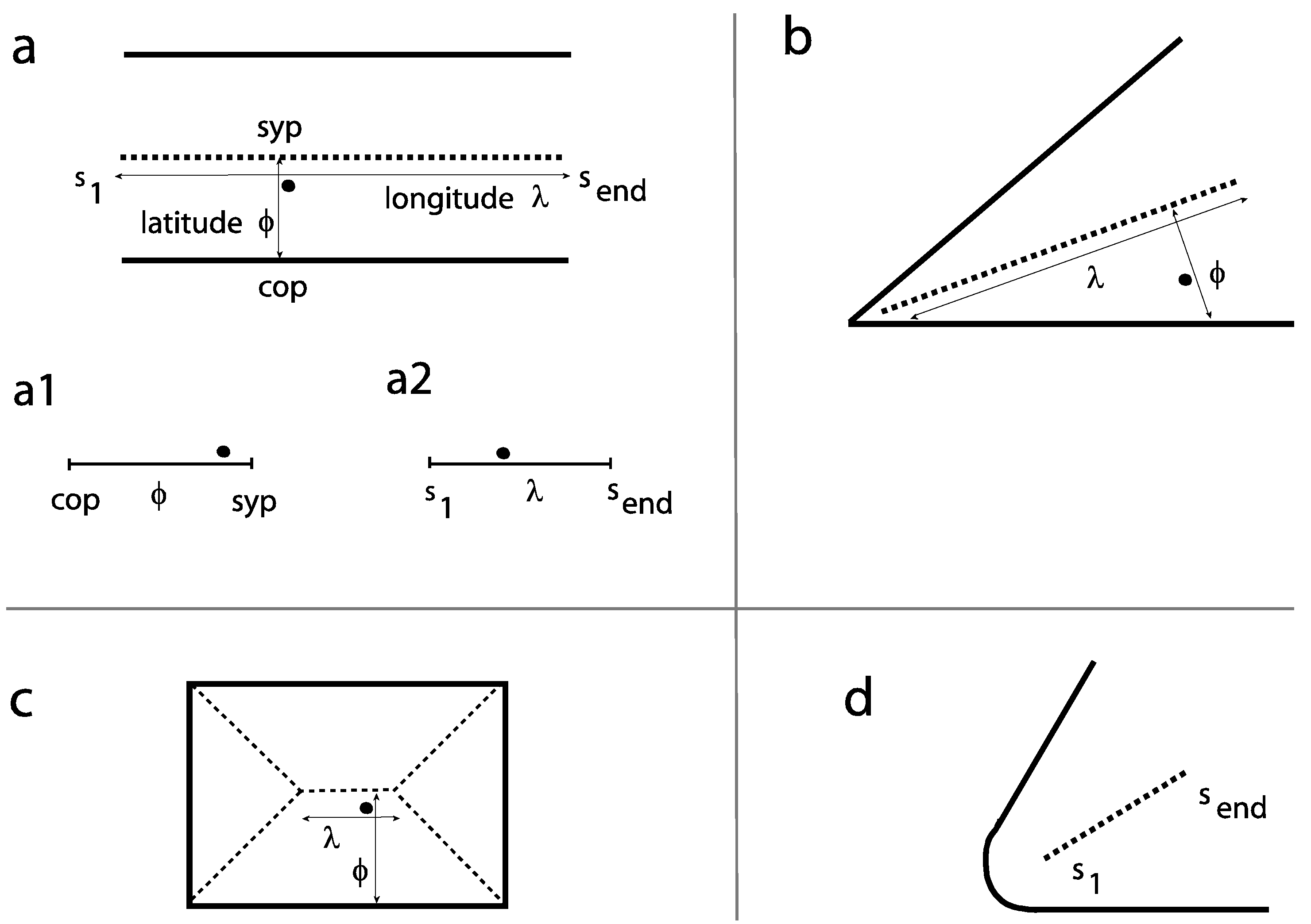
We carry out a systematic analysis for a set of different levels of the fine-to-coarse scale. For each level of the fine-to-coarse scale, the symmetric axes for its contour image are evolved and the relative distances of the fixation locations to the nearest axes are determined. Other key-points (COA, COG) are of limited use in pictures, as closed-contour shapes are rare in gray-scale images. To describe the specific alignment between a fixation point and its region, a fixation is related to its nearest symmetric-axis (sym-axis) segment using two distance measures, the latitude (φ) and the longitude (λ). This is firstly exemplified for two parallel segments (Figure 1a). The latitude describes the displacement between the fixation point and the sym-axis segment and is given as the relative location on a scale ranging from the corresponding pixel on the contour to the symmetric point (sym-point) on the sym-axis. The two ends are abbreviated with 'cop' and ‘syp’ respectively (see subgraph a1). The longitude describes the relative location of the fixation point along the sym-axis segment and is given on a scale ranging from one end to the other (‘s₁’ to ‘s_end’, see subgraph a2). Figure 1b shows the two measures for a fixation point placed in an L feature. Figure 1c shows the example for a fixation point placed in a rectangle; the fixation point is closest to the sym-axis segment representing the two long parallel segments – the determined latitude and longitude measures essentially correspond to the parallel case shown in Figure 1a.

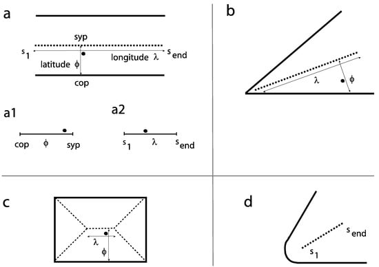
Figure 1. Symmetric axes (sym-axes) and distance measures latitude (φ) and longitude (λ) for a given fixation point (small filled circle). a. Example for two parallel segments: the sym-axis is black dashed. Subgraphs a1, a2: the two scales show how the relative location is denoted in later figures (Figures 3 to 5). b. Example L feature (with sharp corner). c. Example rectangle. The shown fixation point is closest to the sym-axis segment representing the parallel segments. d. The sym-axis segment for a round-corner L feature. s₁ is the initial distance, s_end is the end distance.

Figure 1. Symmetric axes (sym-axes) and distance measures latitude (φ) and longitude (λ) for a given fixation point (small filled circle). a. Example for two parallel segments: the sym-axis is black dashed. Subgraphs a1, a2: the two scales show how the relative location is denoted in later figures (Figures 3 to 5). b. Example L feature (with sharp corner). c. Example rectangle. The shown fixation point is closest to the sym-axis segment representing the parallel segments. d. The sym-axis segment for a round-corner L feature. s₁ is the initial distance, s_end is the end distance.

2. Method

The symmetric-axis transform. There exist different kinds of implementations of the symmetric-axis transform. For instance Feldman and Singh provide an implementation which aims at a precise description of complex areas (2006), but which operates only on closed shapes. In this study, the SAT is rather used as in Blum’s original proposal (1967, 1973), namely as a method to determine the region outlined by an arbitrary structure (open shapes included). Our implementation is best demonstrated by looking at its output.

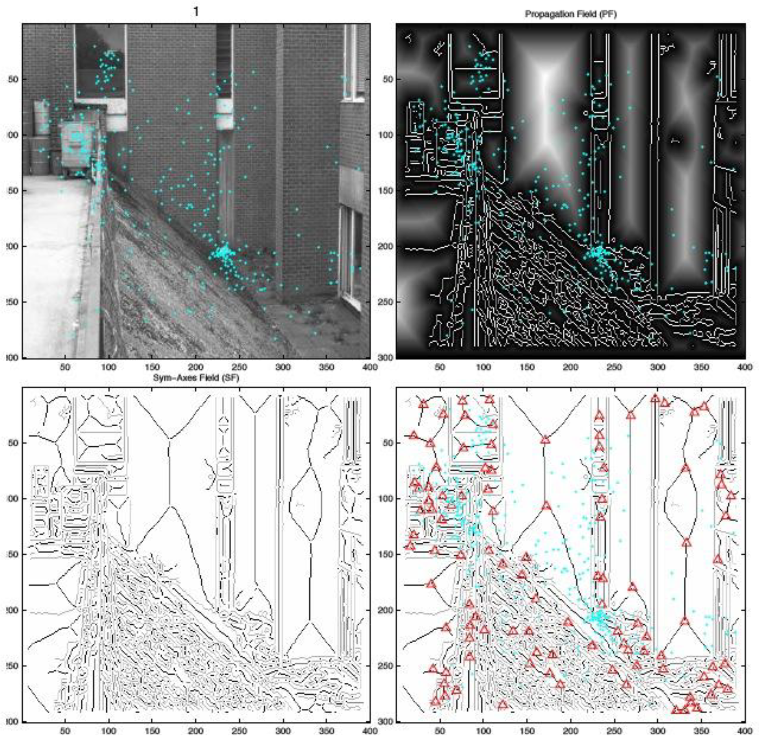
The first step is to let the contours of a binary edge image propagate until all contours have collided. The temporal evolvement of this propagation process is held as scalar values in a 2D map,the distance map DM, in which each pixel represents the time stamp when a propagating contour has passed. For a rectangle, DM has the shape of a roof; for a circle it has the shape of a cone. The distance map is shown in the upper right of Figure 2; increasing luminance values correspond to temporal evolvement. The sym-axes can already be recognized as ‘veins’ running through the regions. The DM can be regarded as a landscape, in which contours run like rivers through the valley bottom and crests (or ridges) of the hills correspond to the symmetric axes. No plateaus are existent in the distance map.For a model generating the distance map DM we refer to Rasche (2007). It is only pointed out that the temporal evolvement of DM is strongly quantized due to its implementation. This quantization can be observed for the large, near-rectangular region in the center or the top half of Figure 2, where the brightness values evidently increase in a pyramidal fashion.

The second step is to detect and extract the sym-axes from the distance map, for which DM is convolved with a high-pass filter resulting in an image with emphasized veins. Subsequent thresholding and thinning results in the sym-axis as shown in Figure 2 lower left. The strength of our implementation is that it is largely robust to contour fragmentation: small contour gaps are sealed during the propagation process but they also generate a short symaxis.Sym-axes segments are only evolved if the propagating contours meet at an angle smaller than ca. 135 degree in our implementation.

A downside of the symmetric-axis transform is that it is susceptible to noise: speckled or spurious contour streaks can lead to 'distorted' axes, see for example the sym-axis for the long vertical wall surface in the in right of Figure 2 (between y=300 and y=370). It is very difficult to eliminate such noise, as it essentially corresponds to an attempt to solve the issue of image segmentation. Nevertheless, the symmetric axes obtained from different scales can be very representative, as we have shown in an image classification study using different image collections (Rasche, 2010).

Sym-axes segments. The sym-axes are then segregated into its constituent sym-axis segments at points of intersections (marked as red plus signs in Figure 2, lower right). For instance, the sym-axes of a rectangle are segregated into 5 segments (Figure 2c), of which 4 segments describe the corresponding L-features and one segment describes the central segment expressing the rectangle's long sides. The values of the sym-axis segment, s(v), correspond to values in the distance map DM , where v is the arc length variable. For a L feature, the segment values s are continuously increasing, for a pair of parallel segments they are constant.

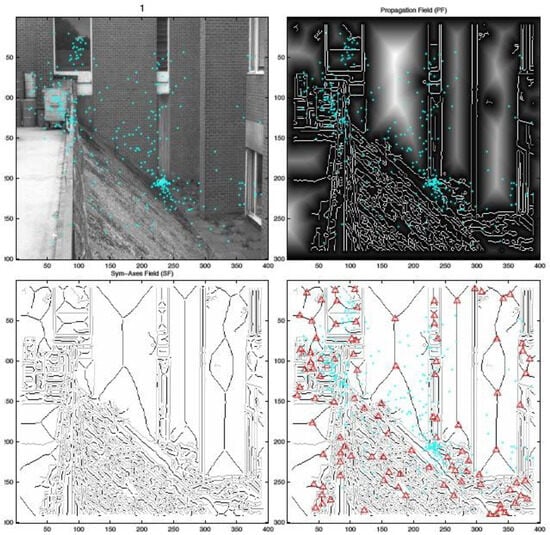
Figure 2. Example of a symmetric-axis transformation of a contour image (cyan dots denote fixation locations for 22 subjects for the first 5 seconds of viewing; image taken at 3^rd scale (I₃). Upper right: Distance mapwith symmetric axes already visible as veins in the regions (contours in white; regions are bright). Lower left: Contours (gray) and symmetric axes (black), respectively. Lower right: Intersections of sym-axes segments marked with red plus signs.

Figure 2. Example of a symmetric-axis transformation of a contour image (cyan dots denote fixation locations for 22 subjects for the first 5 seconds of viewing; image taken at 3^rd scale (I₃). Upper right: Distance mapwith symmetric axes already visible as veins in the regions (contours in white; regions are bright). Lower left: Contours (gray) and symmetric axes (black), respectively. Lower right: Intersections of sym-axes segments marked with red plus signs.

Because many segments show increasing distance values (e.g., L feature, converging segments), the terms initial and end symmetric distance are used to denote the beginning and end of a segment, s₁ and s_end respectively (see Figure 1d). For two exactly parallel segments they are equal (s₁=s_end). From these two values the approximate angle of the L feature can be calculated. The minimum width of a sym-axis segment is defined as 2·min_v(s(v)) and equals 2·s₁ in case of an L feature.

Latitude and Longitude. The latitude φ can be determined by exploiting the distance map DM and is defined as ranging from 0 to 1. For a given fixation i_fix and its nearest segment s_near, the relative distance φ to the nearest point v_near on the sym-axis is taken: φ = DM(i_fix)/s_near(v_near). If the fixation lies exactly on a contour pixel then φ is 0 (DM = 0 for contour pixels); if the fixation lies exactly on a sym-axis pixel, then φ is 1, as DM(i_fix) = s_near(v_near). The longitude is computed by finding the closest sym-point (shortest distance) on the nearest sym-axes segment s_near and determining the point's relative location on its segment; the measure also ranges from 0 to 1.

Images &fixation data. The dataset from Tatler & Vincent (2009) was employed. It consists of recordings of 22 subjects viewing 120 color images, each for 5 seconds. Each high-resolution image subtended 40 degrees horizontally and 30 degrees vertically. A total of ca. 40000 fixations were collected. To obtain a set of random fixation locations for a given participant viewing a given image, all fixation locations made by that participant on all other images were used to construct an overall distribution, from which a set of locations was randomly sampled. This technique means that image-independent sampling biases displayed by an individual do not confound the comparison between fixated and control locations (Tatler et al., 2005). For each image I₁, a pyramid of five down-sampled images was generated, taking half the resolution for successive higher levels (I₂, …, I₅). To obtain the (binary) contour image, each level of the pyramid was processed with the Canny algorithm at the finest scale (σ=1). Later, the term scale refers solely to the pyramid and not the sigma value of the Canny algorithm. How the sym-axes appear for different spatial scales is shown in our previous publication (Rasche, 2010).

3. Results

A first step is to look at the latitude histogram for fixations that landed in large regions (Figure 3), for which sym-axes with a minimum width of 3.0 degrees of visual angle are selected. This selection is geometrically unspecific, but allows to understand the distribution for more specific features. The x-axis corresponds to the chosen distance definition, ranging from the contour pixel (value=0) to the sym-point on the nearest sym-axis segment (value=1, see also Figure 1, subgraph 1a). The random distribution monotonically decreases and is not a constant distribution dueto the fact that the area around sym-axes segments is smaller than the entire area. To clarify, consider rings (annuli) with increasing radius but with the same width (between the concentric circles): for increasing radius the area increases too and leads therefore to a larger sampling. The actual (human) distribution starts slightly higher than the random distribution, but decreases faster and then remains below the random distribution. The statistical difference between the two average distributions is often highly non-significant (t-test; p>0.9).

In order to emphasize potentially preferred locations of human target selection, the positive difference between the two distribution is taken (actual minus random; shown in blue), which is hereafter called the preference distribution. It is emphasized that this distribution shows only preferred locations and not an absolute proportion of fixations. The preference distribution in Figure 3 is elevated near the contour (φ<0.3), indicating that a fixation tends to lie closer to the nearest contour than to the nearest sym-axis segment. This finding of contour preference is consistent with previous reports that edge information offers some predictive power for fixation placement (Baddeley and Tatler, 2006).

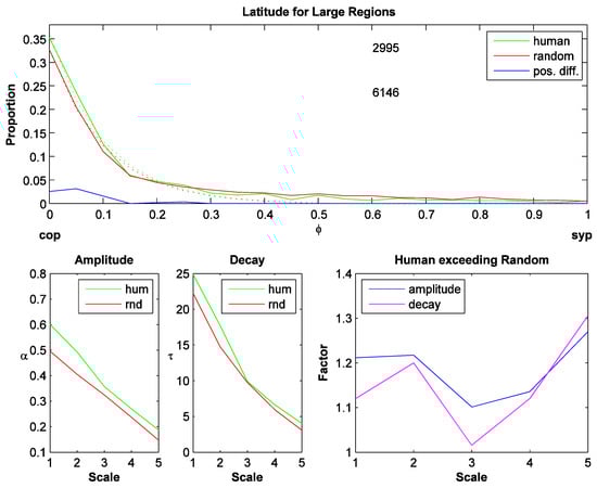
Figure 3. Latitude for large regions (sym-axes with high DM value). Top plot: Latitude histogram for scale 3. X-axis: Latitude: ranges from contour pixel (cop; value=0) to sym-point (syp; value=1). Green: human fixations; red: random fixations; blue: preference distribution: positive difference of actual (human) distribution minus random distribution. The two numbers denote the number of human and random fixations for each selection (upper and lower respectively). The dotted curves are exponential fits (αe^(-τφ)). Lower left two plots: amplitude (α) and decay rate (τ) of the fits for the 5 different scales (I₁,…, I₅). Lower right plot: Factor by which the actual distribution exceeds the random distribution (α_hum/α_rnd and τ_hum/ τ_rnd).

Figure 3. Latitude for large regions (sym-axes with high DM value). Top plot: Latitude histogram for scale 3. X-axis: Latitude: ranges from contour pixel (cop; value=0) to sym-point (syp; value=1). Green: human fixations; red: random fixations; blue: preference distribution: positive difference of actual (human) distribution minus random distribution. The two numbers denote the number of human and random fixations for each selection (upper and lower respectively). The dotted curves are exponential fits (αe^(-τφ)). Lower left two plots: amplitude (α) and decay rate (τ) of the fits for the 5 different scales (I₁,…, I₅). Lower right plot: Factor by which the actual distribution exceeds the random distribution (α_hum/α_rnd and τ_hum/ τ_rnd).

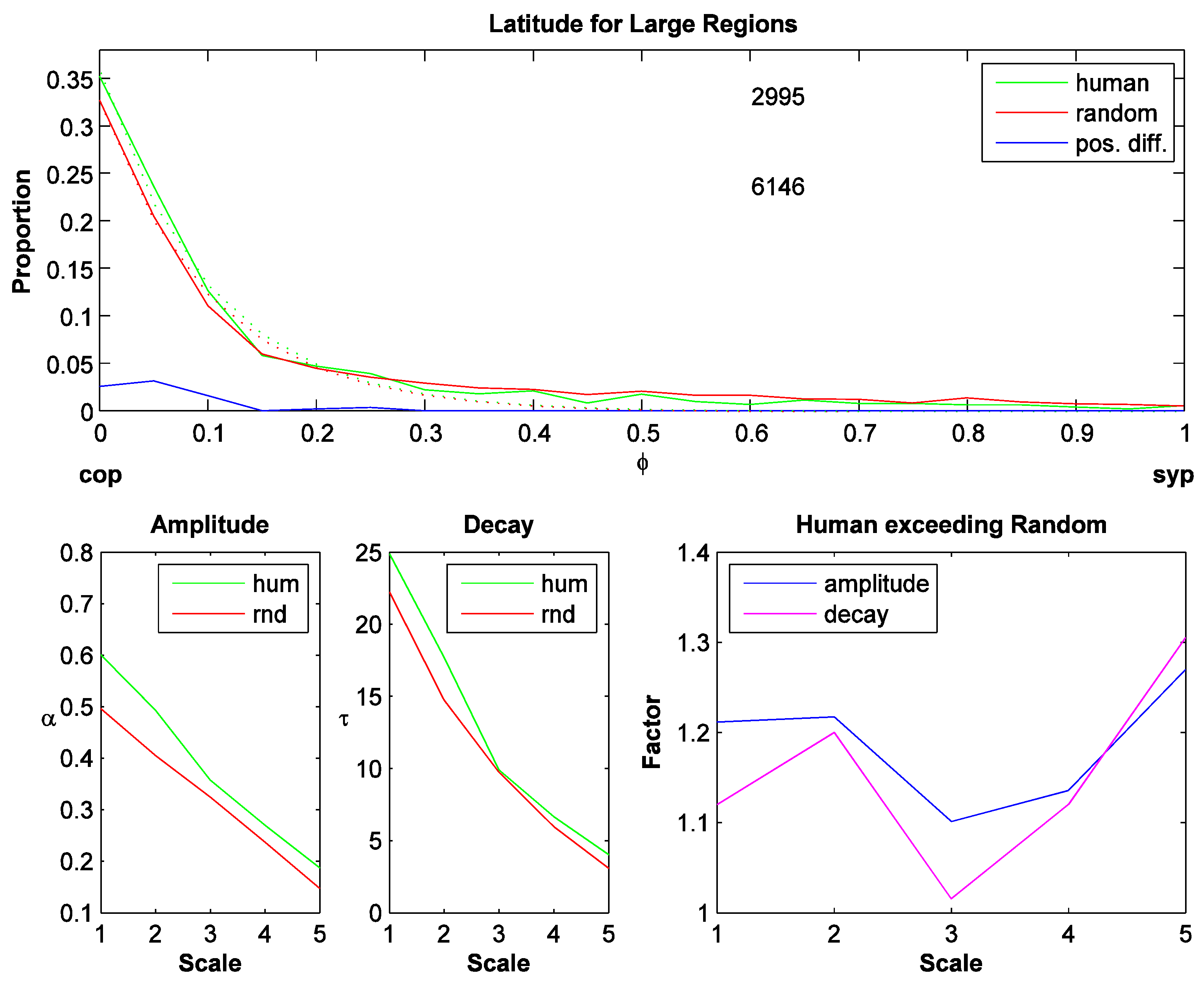
The preference distributions look similar for different scales but change systematically in their amplitude and their decay rate. This is estimated by fitting an exponential function to each distribution,αe^(-τφ) , where α is the amplitude and τ is the decay rate. The lower left two plots in Figure 3 show that the amplitude and the decay rate decrease for coarser scales. To compare the actual against the random distribution, the fitted parameter values are divided: f_α=α_hum/α_rnd and f_τ=τ_hum/ τ_rnd (actual divided by random; lower right plot, Figure 3). These 'factors' are largest for the coarsest scale indicating that on the coarsest scale, fixations are placed even closer to the contour than on a finer scale. The bin size was 20 for these histograms, but when small sym-axes are included, the distributions become quantized due to the technique generating the distance map. Later preference distributions are therefore generated with 10 bins only and to compare with other distributions, the preference distribution for large regions is generated with 10 bins and averaged across all scales. The resulting scale-averaged preference distribution is shown in Figure 4a. The scale-averaged preference distribution for small regions is shown in Figure 4b: it has a larger variance and shows a shift toward the right. The two preference distributions are statistically not different (t-test, p=0.529).

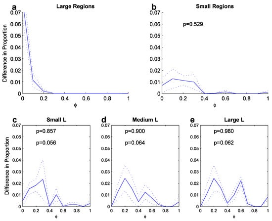
Figure 4. Latitude preference distributions (averaged across scales; dotted curves outline width of standard deviation). X-axis as in Figure 3 top plot. a. Large regions. b. Small regions. c-e. Preference for L features for three angle bandwidths (small [0, 17], medium [18, 45] and large [46, 135] angles; unit in degrees). Top p-value: t-test with distribution in a; Bottom p-value: t-test with distribution in b.

Figure 4. Latitude preference distributions (averaged across scales; dotted curves outline width of standard deviation). X-axis as in Figure 3 top plot. a. Large regions. b. Small regions. c-e. Preference for L features for three angle bandwidths (small [0, 17], medium [18, 45] and large [46, 135] angles; unit in degrees). Top p-value: t-test with distribution in a; Bottom p-value: t-test with distribution in b.

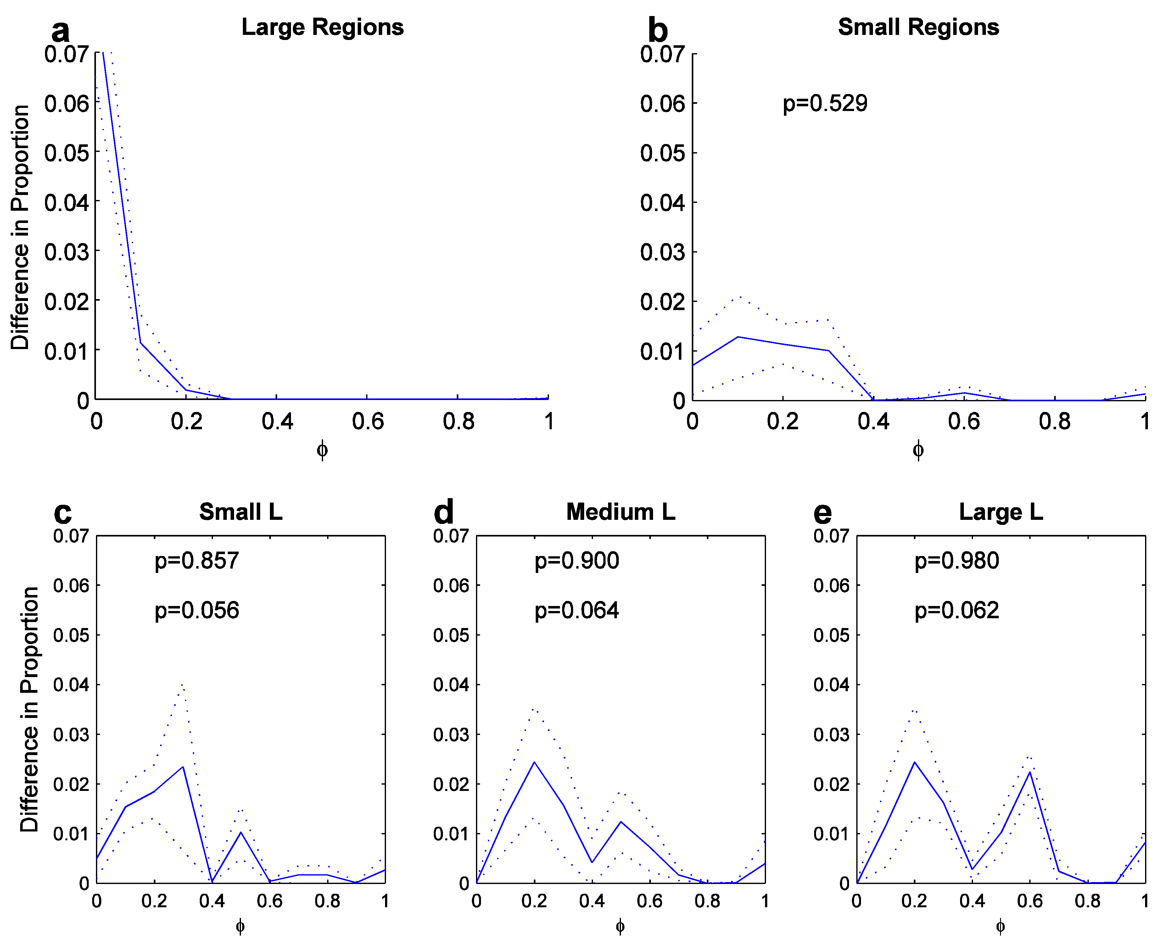
As a large number of sym-axes segments represent L features, they are investigated next. Figure 4c-d shows (scale-averaged) latitude-preference distributions for L features for three disjoint angle bandwidths averaged across scales. The angle bandwidths cover the ranges [0, 17], [18, 45] and [45, 135] degrees, called small, medium and large respectively. Larger angles are not generated by the symmetric-axis transform. Because sharp-cornered L features, such as the one depicted in Figure 1b (s₁=0 theoretically) are rare, we included also sym-axes representing round-cornered L features such as the one depicted in Figure 1d, for which the sym-axis starts with some delay (s₁>0). The conditions for L-feature selection were: a) a maximal, initial symmetric-distance value of s₁<0.2·l_seg, whereby l_seg is the total arc length of sym-axis segment; b) a minimum length of the sym-axis segment, which was larger than the minimum symmetric distance: lseg>s1.

For each bandwidth, the scale-averaged preference distribution appears as shifted toward the side of the symaxis, in comparison to the distribution for small regions. Each L-feature distribution is individually compared to the distribution for large and small regions by a t-test (values also given in each plot; upper and lower respectively): the L-feature distributions are hardly different in comparison to the one for large regions (p=0.857, p=0.900 and p=0.980), but they are significantly different in comparison to the one for small regions on a 10-percent level (p=0.056, p=0.064 and p=0.062). Thus, for L features there appears to be a shift away from the contour and toward the nearest sym-axis. There even appears to be a slight shift toward the sym-axis segment when one compares the distributions for increasing angle (c to e): the 2nd peak (at ca. φ =0.5) increases slightly.

We also generated latitude preference distributions for the intersection points of the sym-axis (red plus signs in Figure 2, lower right graph). This represents a more direct measure of whether fixations are drawn to the center of a region. The distributions were generated for small and large regions but looked very similar to the ones shown in Figure 4a and 4b and are therefore not shown.

We now turn toward the longitude measure, which is determined for a variety of structures (Figure 5). It is determined only for ‘elongated’ sym-axes segments, whose arc length is larger than a minimal spatial width of the region, which here is chosen to be the initial symmetric distance, l_seg>=s₁; without such a minimal elongation, the longitude measure makes little sense. Figure 5a displays the scale-averaged preference distribution for all elongated segments, showing a noisy but gradual decay along the axis from s₁ to s_end, meaning there is a fixation bias towards the narrower part of a region. For parallel segments with a maximum angle of 3 degrees (straight or curved), the distribution is slightly more spread (Figure 5b), covering the entire axis range. The distribution is statistically not different to the distribution for all elongated regions in Figure 5a (t-test, p=0.368).

In an attempt to elucidate significant differences, the parallel-structure fixations were separated into two groups according to their degree of latitude: those that landed nearer to the contour (φ<0.5; Figure 5c) and those that landed nearer to the sym-axis segment (φ>=0.5; Figure 5d). The preference distribution for both are higher in comparison to the general distribution in Figure 5b. The near-contour distribution shows an increase toward either half of the parallel structure, in comparison to the general distribution, but the two distributions are statistically not different (t-test, p=0.189). The near-sym-axis distribution shows and increase in its central part of the axis range and the distribution was statistically different from the general distribution (t-test, p=0.032). The two distributions, near-contour versus near-sym-ax, were not significantly different from each other (t-test, p=0.318; value not shown in plots). A number of other (scale-averaged) preference distributions were analyzed, such as the latitude distribution for parallel contours and the longitude distributions for vertical and horizontal parallel contours. But none of these showed any biases or particular differences amongst each other.

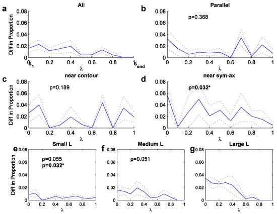
Figure 5. Longitude preference distribu-tions (averaged across scales; dotted curves outline width of standard deviation). X-axis: from s₁ (0) to s_end (1).a. Preference for all fixations near elongated sym-axes. b. Preference for parallel sym-axes. c. Preference for fixations near contour. d. Preference for fixations near sym-axes. e.-g. Longitude preference for L features of three angle bandwidths (angle bandwidths).

Figure 5. Longitude preference distribu-tions (averaged across scales; dotted curves outline width of standard deviation). X-axis: from s₁ (0) to s_end (1).a. Preference for all fixations near elongated sym-axes. b. Preference for parallel sym-axes. c. Preference for fixations near contour. d. Preference for fixations near sym-axes. e.-g. Longitude preference for L features of three angle bandwidths (angle bandwidths).

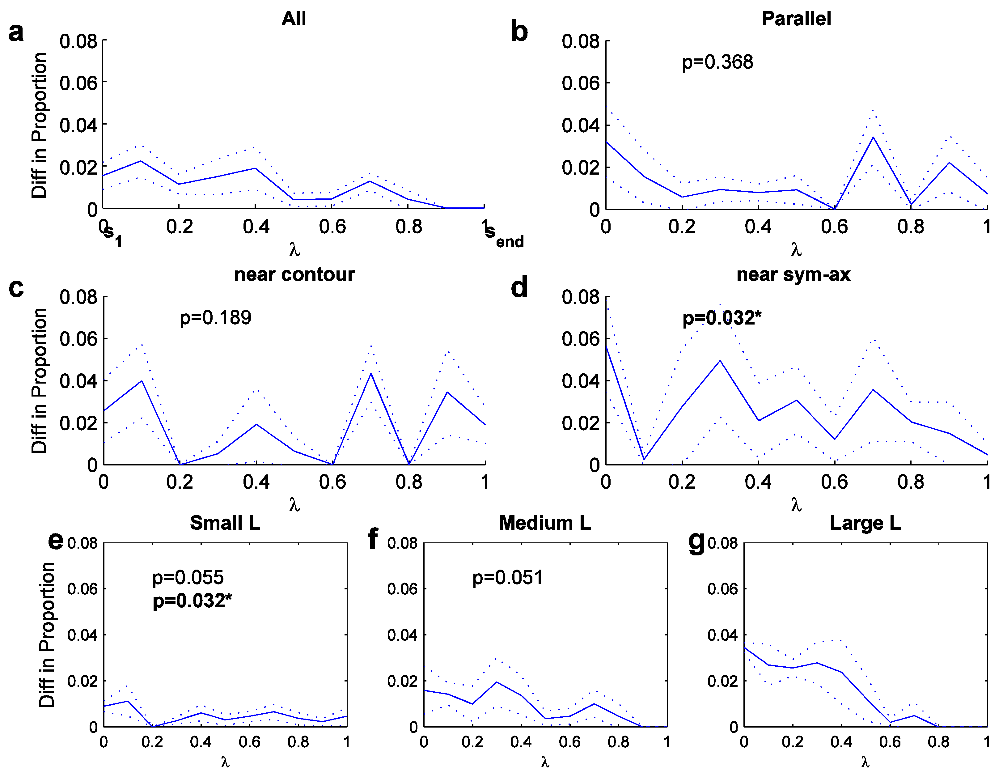
But further significances can be found when looking at the average longitude preference distribution for L features (Figure 5e-g), for which the same angle bandwidths were used as before. For small angles, the distribution is similar to the one for parallel segments due to their structural similarity: the distribution covers the entire range. But for increasing angles (Figure 5f and g), the distribution shifts toward zero, meaning for larger angles fixation in the corner is preferred. The statistical difference between the small and the medium, and the medium and the large L-feature distribution was marginal (t-test; p=0.055 and 0.051), but the one between small and the large was significantly different at a 5 percent level (p=0.032). Summarized, there seems to exist a progression from placing the fovea to the open side for small-angled L features, to placing it to toward the corner for large-angled L features.

A number of other preference distributions were analyzed, whose choice is partly motivated by results of studies analyzing fixation behavior in real-world scenes. Previously, it was shown that short- and long-range saccades showed differential extents of correlation between fixation placement and basic image features (Tatler, Bad-deley and Vincent, 2006). We therefore compared fixation placement with respect to structural features after small (<3 degrees) and larger (> 6 degrees) saccades were made. However, no differences were apparent for latitude distributions for fixations following small or large saccades. Given previous suggestions that after the onset of a new scene, the early portion of viewing is quantifiably different from later viewing (e.g., Parkhurst et al., 2002; Tatler et al., 2005) and may be about gathering structural information about a scene (e.g., Buswell, 1935), we also partitioned our data into early and late saccades (<750ms and >3500ms since stimulus onset). However, the latitude distributions did not show particular differences either.

4. Discussion

For L features of small angle, the longitude measure suggested that fixations tended to be placed in the open side (Figure 5e). The corresponding latitude measurement suggests that the fixations are preferably placed just next to the contour (Figure 4c). This fixation bias is almost identical to what has been measured as fixation distributions for isolated, small-angled L features by Richards and Kaufman (their Figure 1 in 1969). For increasing angles the fixations shifted toward the corner and for large angles some fixations are even placed in the apex (Figure 5g). That fixations are sometimes exactly placed in the apex was also observed for some subjects in Richards and Kaufman's study (Richards and Kaufman, 1969), but also in studies in which the task was to count the number of corners of a polygon (Guez et al. 1994). There exists the possibility that in our study a L feature is part of a vertex feature (three intersecting contours), but such features are rare in contour images and no attempt was made to distinguish between vertex and L features.

For parallel structures, the longitude preference distribution in Figure 5b suggests that fixations tended to be placed toward either half of the elongated structure. But analyzing these fixations in more detail, by splitting them into the ones that landed either nearer the contour or nearer the sym-axes (Figure 5c and d), draws a more discerned picture of fixation behavior. If fixations had landed closer to the sym-axis, than there is a landing bias toward the middle of the sym-axis. If fixations had landed closer to the contour, then there is a bias toward either half. Thus, if one regards a parallel segment as a rectangle, whose ends are connected, then there exists a trend to fixate either the corners of the rectangle or its center.

It should be emphasized again, that our analysis has uncovered trends only by using the difference between the actual and a random distribution. No absolute distributions of fixation positions were shown in figures 4 and 5. Still, the tendencies we have found, support the findings by Kaufman and Richards (1969), who suggested that fixation locations are associated with the symmetric axis transform. However, Kaufman and Richards did not provide a detailed model of how exactly the fixation points are determined using the sym-axes. Other studies have found that saccades land closer to the COG of linedrawing shapes or of cluster of dots (Melcher and Kowler, 1999); or target selection is determined by luminance contrast when counting corners of a polygon (Guez et al, 1994). One reason for the variety of findings is that the studies use different shapes and task instructions. For instance in Melcher and Kowler’s study, the subject is asked to carry out a primary saccade toward a complex structure. In such situations there may indeed be a preference to place the fovea on the COA. This mechanism may also function during free-viewing as well, but we have not yet attempted to find such a preference. The reason is that it is difficult to extract the exact outline of a region (from a gray-scale image) for a shape which is more complex than just an L feature or parallel structure. A caveat to consider is that there may be multiple mechanisms at work simultaneously which are given different priority depending on the context of the structure and of the task.

In the present study we found significant differences between actual and control fixation locations, which point toward a role for structural analysis in saccade target selection. However, it should be noted that in most cases, significance testing shows that these differences tend to be significant at and around the 5% or 10% level. These statistical differences are modest compared to those typically observed between fixated and control locations for low-level image features (e.g., Tatler et al., 2005). Moreover, statistical significance should not be taken as the sole criterion for deciding whether any given factor plays any causal role in fixation selection. As in the case of low-level features in previous studies, what we find is a correlation between structural analysis and fixation placement. However, the present results still offer a first indication that there may be a role for the types of structural analysis we have considered when viewing natural scenes. Further research is required to consider the behavioral (rather than statistical) significant of this finding.

A question which is rarely asked is what is the purpose of those specific fixation locations? Because structure can be recognized independent of its spatial location (translation independent), one may wonder why those preferred fixation locations exist at all. They may exist for various purposes such as accurate spatial measurement to determine the precise relation between contours, objects or scene parts. Viewing experiments with specific task instructions may provide answers to that question. Another question is how those points are computed accurately. It is only Guez et al. (1994) who give a precise model for their corner-counting task. But the computation of a COA is not as easy to achieve as it seems – in particular in non-segmented scenes. It is actually the sym-axes themselves which can deliver such a point, as they describe the region by their distance values. Thus, the symaxes themselves may not be the saccadic target, but they may be used for computing more specific targets.

There are a number of reasons why it is difficult to assess the exact extent to which structural analysis is involved in fixation placement. One difficulty is to determine the exact point of saccadic target selection for two reasons: measurement error and the saccadic amplitude variability. The measurement error of the eye-tracker is approximately 0.5 degrees, a general lower limit of eyegaze recordings (Wade and Tatler, 2005). How precisely saccades land on their intended target is also hard to assess in complex scenes, where the target is not known. In simplified tasks using isolated targets, saccades tend to fall short of their intended target by about 8-10% (Becker, 1972; Henson, 1997). Melcher and Kowler (1999) compensated for that variability in some of their analysis by measuring the error for individual subjects using a circle. Whether hypometria is a feature of complex-scene viewing is uncertain, but some supportive evidence that this may be the case, has been reported by Tatler and Vincent (2008). These sources of variability in the measured saccade targeting complicate any attempts to relate fixation placement precisely to key points in images of natural scenes.

Another complicating issue is the circumstance that saccades do not necessarily need to land precisely on a target object because the parafovea can sometimes provide enough information for recognition (Rayner 1998; Kirchner and Thorpe 2006; Rasche and Gegenfurtner 2010). Johansson et al. (2001) used a task in which a block had to be moved past an obstacle and brought into contact with a target object. They found that getting the fovea anywhere within a 1.5 degree radius of the obstacle was sufficient to provide the information needed to avoid it and did not require corrective saccades to refine fixation placement. This result supports the idea that foveal targeting need not always precisely bring the fovea onto an object in a complex scene if parafoveal information is sufficient. Thus, it suffices for a (primary) saccade – with the purpose of identifying a piece of structure - to land in its approximate neighborhood. This constitutes in some way an uncertainty principle of anchoring a fixation location to its exact intended saccadic target position.

Can the findings here be used to make better fixation predictions as for instance a discrimination between a fixated patch and a randomly selected patch? Possibly. There are a number of studies performing such a prediction which can be divided into two types. One type pursues a statistical search, such as the original study by Reinagel and Zador (1999), or the support-vector machine approach by Kienzle et al (2006). The other type performs a preprocessing of the image akin to the early visual system using simple features, such as orientation, blob and color (Itti and Koch, 2001; Tatler et al 2005). However, such a free-viewing prediction will always be limited for two reasons. One is the just-mentioned uncertainty principle of anchoring the fixation point, which therefore does not allow for an exact comparison between different observers or between observer and model. The other reason is the individuality of the human observer, an issue which contributes even more to the difficulty of making comparisons.

But it is the study by Kienzle that showed an interesting computational result. In Kienzle’s study (2006) the goal was to find possible saccadic targets using the classification method of support-vector machines. One major finding was that the ideal fixation patch is a centersurround structure akin to the receptive field of the early visual pathway, which is not a very specific finding with regard to the precise saccadic target mechanism. It is rather their Figure 4b – showing the most effective set of all actual optimal fixation patches – that the foveated loci are structures such as vertices, corners, parallel contours and so on. It is therefore worth pursuing models that are much more explicit in their structural analysis than the models performing feature extraction of orientations only (Rasche, 2010). Combined with our findings of structural specificity for L features and parallel features, this may lead to a better discrimination of fixated and random patches.

References

- Baddeley, R. J., and B. W. Tatler. 2006. High frequency edges (but not contrast) predictwhere we fixate: a Bayesian system identification analysis. Vision Research 46: 2824–2833. [Google Scholar] [CrossRef] [PubMed]
- Becker, W. 1972. The control of eye movements in the saccadic system. Bibliotheca Ophthalmologica 82: 233–43. [Google Scholar]
- Blum, H. 1973. Biological shape and visual science.1. Journal of Theoretical Biology 38, 2: 205–287. [Google Scholar] [CrossRef] [PubMed]
- Blum, H. 1967. A new model of global brain function. Perspectives in Biology and Medicine 10, 3: 381–408. [Google Scholar] [CrossRef]
- Einhauser, W., M. Spain, and P. Perona. 2008. Objects predict fixations better than early saliency. Journal of Vision 8, 14: 11–26. [Google Scholar] [CrossRef] [PubMed]
- Feldman, J., and M. Singh. 2006. Bayesian estimation of the shape skeleton. Proceeding of the National Academy of Sciences USA 21 103, 47: 18014–18019. [Google Scholar] [CrossRef]
- Groner, R., F. Walder, and M. Groner. 1984. Edited by A.G. Gale and F. Johnson. Looking at faces: Local and global aspects of scanpaths. In Theoretical and applied aspects of eye movement research. Amsterdam: Elsevier North-Holland, pp. 523–533. [Google Scholar]
- Guez, J. E., P. Marchal, J. F. Le Gargasson, Y. Grall, and J. K. O'Regan. 1994. Eye fixations near corners: evidence for a centre of gravity calculation based on contrast, rather than luminance or curvature. Vision Research 34, 12: 1625–35. [Google Scholar] [CrossRef]
- Henson, D. B. 1979. Investigation into corrective saccadic eye movements for refixation amplitudes of 10 degrees and below. Vision Research 19, 1: 57–61. [Google Scholar] [CrossRef]
- Johansson, R. S., G. R. Westling, A. Backstrom, and J. R. Flanagan. 2001. Eye-handcoordination in object manipulation. Journal of Neuroscience 21, 17: 6917–6932. [Google Scholar] [CrossRef]
- Itti, L., and C. Koch. 2001. Computational modelling of visual attention. Nature Reviews Neuroscience 2, 3: 194–203. [Google Scholar] [CrossRef]
- Kaufman, L., and W. Richards. 1969. Spontaneous fixation tendencies for visual forms. Perception & Psychophysics 5, 2: 85–88. [Google Scholar]
- Kirchner, H., and S. J. Thorpe. 2006. Ultra-rapid object detection with saccadic eye movements: Visual processing speed revisited. Vision Research 46: 17621776. [Google Scholar] [CrossRef]
- Locher, P., D. Cavegn, M. Groner, P. Mueller, G. d’Ydewalle, and R. Groner. 1993. The effects of stimu-lus symmetry and task requirements on scanning patterns. In Perception and cognition: Advances in eye movement research. Edited by G. G. d’Ydewalle and J. van Rensbergen. Amsterdam: Elsevier, pp. 59–69. [Google Scholar]
- Melcher, D., and E. Kowler. 1999. Shapes, surfaces and saccades. Vision Research 39: 2929–2946. [Google Scholar] [CrossRef]
- Menz, C., and R. Groner. 1985. The effect of stimulus characteristics, task requirements and individual differences on scanning patterns. In Eye movements and human information processing. Edited by R. Groner, G. W. McConkie and Ch Menz. Amsterdam: Elsevier-North Holland, pp. 239–250. [Google Scholar]
- Noton, D., and L. Stark. 1971a. Scanpaths in saccadic eye movements while viewing and recognizing patterns. Vision Research 11: 929–942. [Google Scholar] [CrossRef]
- Parkhurst, D. J., K. Law, and E. Niebur. 2002. Modeling the role of salience in the allocation of overt visual attention. Vision Research 42, 1: 107–123. [Google Scholar] [CrossRef] [PubMed]
- Treisman, A., and S. Gormican. 1988. Feature analysis in early vision: Evidence from search asymmetries. Psychological Review 95, 1: 15–48. [Google Scholar] [CrossRef]
- Rasche, C. 2007. Neuromorphic Excitable Maps for Visual Processing. IEEE Transactions on Neural Networks 18, 2: 520–529. [Google Scholar] [CrossRef] [PubMed]
- Rasche, C. 2010. An Approach to the Parameterization of Structure for Fast Categorization. International Journal of Computer Vision 87: 337–356. [Google Scholar]
- Rasche, C., and K. Gegenfurtner. 2009. Accuracy of Speed Discrimination and Smooth Pursuit Eye Movements. Vision Research 49: 514–523. [Google Scholar] [CrossRef]
- Rasche, C., and K. Gegenfurtner. 2010. Orienting during Gaze Guidance in a Letter-Identification Task. Journal of Eye Movement Research 3, (4):3: 1–10. [Google Scholar] [CrossRef]
- Rasche, C., and C. Koch. 2002. Recognizing the Gist of a Visual Scene: Possible Perceptual and Neural Mechanisms. Neurocomputing (44-46): 979–984. [Google Scholar]
- Rayner, K. 1998. Eye movements in reading and information processing. 20 years of research. Psychological Bulletin 124: 372–422. [Google Scholar] [PubMed]
- Reinagel, P., and A. M. Zador. 1999. Natural Scene statistics at the centre of gaze. Network: Computation in Neural Systems 10: 341–350. [Google Scholar]
- Richards, W., and L. Kaufman. 1969. ‘Center of gravitiy’ tendencies for fixations and flow patterns. Perception and Psychophysics 5: 81–84. [Google Scholar]
- Tatler, B. J., R. J. Baddeley, and B. T. Vincent. 2006. The long and the short of it: Spatial statistics at fixation vary with saccade amplitude and task. Vision Research 46: 1857–1862. [Google Scholar]
- Tatler, B. W., R. J. Baddeley, and I. D. Gilchrist. 2005. Visual correlates of fixation selection: Effects of scale and time. Vision Research 45: 643–659. [Google Scholar] [CrossRef]
- Tatler, B. W., and B. T. Vincent. 2008. Systematic tendencies in scene viewing. Journalof Eye Movement Research 2(2), 5: 1–18. [Google Scholar] [CrossRef]
- Tatler, B. W., and B. T. Vincent. 2009. The prominence of behavioural biases in eyeguidance. Visual Cognition 17, 6-7: 1029–1054. [Google Scholar]
- Thorpe, S. J., D. Fize, and C. Marlot. 1996. Speed of processing in the human visual system. Nature 381: 520–522. [Google Scholar]
- Torralba, A., A. Oliva, M. S. Castelhano, and J. M. Henderson. 2006. Contextual guidance of eye movements and attention in real-world scenes: The role of global features in object search. Psychological Review 113, 4: 766–786. [Google Scholar]
- Marsman, J. B.C, V. Yanulevskaya, and F. W. Cornelissen. 2007. Spatial statistics of natural images predict gaze direction. Perception 36: 35–36. [Google Scholar]
- Wade, N. J., and B. W. Tatler. 2005. The Moving Tablet of the Eye: the Origins of modern Eye Movement Research. New York: Oxford University Press. [Google Scholar]
- Zelinsky, G. J., and J. Schmidt. 2009. An effect of referential scene constraint on searchimplies scene segmentation. Visual Cognition 17, 6&7: 1004–1028. [Google Scholar] [CrossRef]
Copyright © 2011. This article is licensed under a Creative Commons Attribution 4.0 International License.