Next Article in Journal
The Behavioural and Neurophysiological Modulation of Microsaccades in Monkeys
Previous Article in Journal
Mixed Responses: Why Readers Spend Less Time at Unfavorable Landing Positions
 
 
Journal of Eye Movement Research is published by MDPI from Volume 18 Issue 1 (2025). Previous articles were published by another publisher in Open Access under a CC-BY (or CC-BY-NC-ND) licence, and they are hosted by MDPI on mdpi.com as a courtesy and upon agreement with Bern Open Publishing (BOP).
Article

Time Course and Hazard Function: A Distributional Analysis of Fixation Duration in Reading

1
Department of Psychology & Neuroscience, Box 90085, Duke University, Durham, NC 27708, USA
2
RIKEN Brain Science Institute, Saitama 351-0198, Japan
J. Eye Mov. Res. 2009, 3(2), 1-23; https://doi.org/10.16910/jemr.3.2.3
Published: 22 December 2009

Abstract

:
Reading processes affect not only the mean of fixation duration but also its distribution function. This paper introduces a set of hypotheses that link the timing and strength of a reading process to the hazard function of a fixation duration distribution. Analyses based on large corpora of reading eye movements show a surprisingly robust hazard function across languages, age, individual differences, and a number of processing variables. The data suggest that eye movements are generated stochastically based on a stereotyped time course that is independent of reading variables. High-level reading processes, however, modulate eye movement programming by increasing or decreasing the momentary saccade rate during a narrow time window. Implications to theories and analyses of reading eye movement are discussed.

Introduction

For over a century eye movements have been used to study the time course of reading processes (Huey, 1908; Rayner, 1998, 2009). The time course is often conceptualized (e.g., Engbert, Nuthmann, Richter, & Kliegl, 2005; Reichle, Pollatsek, & Rayner, 2006) – and visualized (e.g., Dambacher & Kliegl, 2007; Sereno & Rayner, 2003) – as a timeline, on which key parameters such as the onset, offset, and duration of a process are marked. Estimating the time course is critical for understanding reading, but making reverse inferences from eye movements to reading processes is not straightforward. This paper introduces a new approach to estimate the time course of a process based on the distribution of fixation duration. I will begin by formalizing the metaphor of a time course, which, in turn, is based on the dichotomy between fixations and saccades in reading.

Fixations, Processes, and Popcorn

During reading the eyes alternate between two states – fixations and saccades. Fixations are periods of time in which the eyes are relatively stationary and the retinal image is clear. Fixations are interrupted by saccades, which are fast, ballistic movements that bring the eyes to different words. This is, of course, an idealization. The distinction between fixations and saccades is often blurred by eye movements during fixations (Carpenter, 1988; Engbert & Kliegl, 2003; Inhoff & Radach, 1998) and equipment limitations (Duchowski, 2003; McConkie, 1981). These issues, however, do not diminish the importance of the fixation-saccade dichotomy in reading research (Rayner, 1998).
Linking fixation duration and reading processes. The present study focuses exclusively on the duration of fixations, which is shown in numerous studies to reflect on-going reading processes (for reviews, see Clifton, Staub, & Rayner, 2007; Rayner, 1998). The basic linking hypothesis in reading eye movement research hardly needs any justifications: if a variable X, which is predicted to affect exclusively a sub-stage of reading, causes a statistically significant change in the average fixation duration, then the process is implicate in the reading. This logic is instrumental in the discovery of numerous factors influencing reading processes and reading eye movement planning (Rayner, 1998).
Questions arise, however, when mean fixation durations are used to estimate the time course of a process. In the simplest case, suppose a reading process X starts at time t1 and ends at t2, and its effect is to lengthen the fixation duration by T milliseconds. Because reading fixation duration varies from less than 100msec to well over 800msec, it is almost certain that some fixations are terminated before t1, some between t1 and t2, and others after t2. Consequently X has no influence in the first case, partial influence on the second, and full impact on the last. The outcome distribution becomes a mixture of the three distributions. The mean fixation duration, which is a weighted average of the three, bears no simple relationship with unknown parameters t1 and t2 and cannot be used to estimate either. What is missing is an explicit linking hypothesis about how events in mental processes are mapped to empirical distributional parameters.
The problem is further complicated if t1 and t2 are allowed to vary randomly. The jittering creates a mixture of distributions that is generally difficulty to disentangle without knowing the distributions of t1 and t2 in the first place. Estimating even the central tendency of these parameters is not a trivial problem under this scenario. The proposal of this paper is to look at an alternative representation of the model – based on the hazard function – that will allow us to estimate the onset and offset of a mental process from the distribution function of empirical fixation duration.
Before introducing the hazard function based approach, let us first look at how conventional linear statistical models such as the ANOVA deal with the aforementioned mixture problem. In a typical fixed-effect model, an observed fixation duration is the sum of three part – a grand mean (also known as the intercept), the unknown constant effect size T, and an error term that is zero mean and independent, identically distributed (i.i.d.) from one fixation to the next. The constant T can be estimated by comparing conditions that does and does not involve the psychological process of interest. Missing from this model, however, are parameters t1 and t2. Indeed, notions of the onset and offset of an effect have no place in ANOVA-type models. The reason is simple: in order to neatly partition variance (or the sum of squares), the “effect” and “errors” must be independent.
This is implied in a fixed-effect model where the effect size is a constant. It is also guaranteed by the i.i.d. assumption in random-effect and mixed-effect models. An onset time, however, implies that the effect is nonexistent prior to t1 and non-zero after it. In other words, the size of the effect is now a function of the random error, in which case the ANOVA model falls apart. By forcing conventional linear models on fixation duration data, we make a compromise – we give up key concepts like the onset and offset of a process, in exchange for a simple, powerful, but possibly biased (see scenarios discussed above) estimator of the effect size T.
The question is whether this tradeoff gets us closer to an understanding of the time course of reading processes. It appears the dominant linear statistical models are fundamentally unequipped to estimate key elements of a time course, and thus leave a large gap between data and theory. There are ways to get around this problem. One approach is to identify the time course using alternative methodologies such as the ERP (see Dambacher & Kliegl, 2007; Sereno & Rayner, 2003). Another is to impose theoretical constraints on the timing and duration of processes, a successful example of which is the E-Z Reader model (Reichle, Rayner, & Pollatsek, 2003; Reichle, Warren, & McConnell, 2009). This paper provides a third alternative, which estimates the time course from the distribution function of eye movements. An analogy may help to illustrate the gist of the proposal here.
Popcorn. Suppose we have two popcorn makers, an old one that heats at a constant rate and a new one that boasts a time-varying heating program – i.e., its power output changes at predestinated times – but its average wattage output is identical between the two machines. With only an unlimited supply of popcorn, how can we verify the “time-varying” claims of the new machine? Comparing the average cooking time says nothing about whether or when the heating function changes over the time course. But listening to the popping noise may. Intuitively, the rate at which popcorn pops should be a function of the instantaneous wattage output.
Though promising, the idea has a number of issues to resolve. First, the intensity of the popping noise may have a nonlinear relationship with the heating function. In this case one can compare the two machines: where the intensity is higher, there must be more heat. But less noise does not always imply less heat. If the new machine cooks faster than the old one, at some point its popping noise will become sparse, simply because there is not much unpopped corn left. A fair comparison requires a relative intensity index, one that scales the noise by how much corn is still unpopped in the machine. Related, this method becomes be less reliable as time goes on, when popping noises will be few and far between. These and other methodological issues will be addressed in this paper.
In this example, the intensity of popping noises is analogous to the rate at which saccades are generated, and the variable heating program stands for the unknown time course of some underlying reading process. If an ongoing reading process influences the instantaneous rate of saccade generation, intuitively one should be able to estimate the onset, duration, and strength of the process by examining the distribution function of fixation duration. This intuition is formalized in the next section.

A Distributional Model of the Time Course of Reading Eye Movements

The gist of the linking hypothesis is straightforward: if a reading process, X, is engaged between t1 and t2, one should observe changes in the intensity of saccades between t1 + δ and t2 + δ, and the variation in intensity should correspond to the time-varying effect of X. The symbol δ is the inherent delay of the oculomotor system, which for the moment is assumed to be an empirical constant and will be revisited in Discussion. The term intensity of saccades is left vague here intentionally because it is the key to the present model. I will define it after laying out the basic notations.
A symbolic sketch. Let λ(t) be a baseline saccadic intensity function, where t ∈ (0, ∞) is the fixation duration, and λ*(t) be the saccadic intensity when the process X is engaged. For the sake of identifying the time course of X, we wish to have a simple relationship between X and λ, such that λ is affected when – and only when – X is engaged. In other words,
Jemr 03 00008 i002
To simplify the notion, let us redefine λ(t) ← λ(t + δ) for the rest of this paper, i.e., the saccadic intensity function λ(t) is time-shifted by δ to removed it from the formula. The desired intensity function now has the form
Jemr 03 00008 i003
If such a λ function does exist, estimating the time course of X is straightforward. The onset and offset of X correspond to the region where λ(t) and λ*(t) differ. The time-varying strength of X is a function of the amount of changes in the saccadic intensity; this could be measured by γ(t) =λ(t) - λ*(t) (the “additive hazards model,” see Aalen, 1989, 1993), γ(t) = λ(t)/λ*(t) (the “proportional hazards model,” Cox, 1972), or some combination of both (see Martinussen & Scheike, 2006).
Assuming a λ function satisfying (2) exists, the new linking hypothesis allows us to estimate (a) if X has any effect, (b) when its effect starts and ends, and (c) how its strength varies with time. If the assumption of conventional linear models holds, i.e., when the onset and offset times span the full range of the distribution, the λ functions will differ throughout the whole range of fixation duration, too, in which case there are no meaningful t1 and t2 to be identified. A key difference between the new proposal and traditional linear models is in the assumption of the amount of jittering of t1 and t2 – the λ function works when distributions of t1 and t2 are narrow compared to the distribution of fixation duration. This is consistent with predictions of major theories of reading eye movements (e.g., Engbert, et al., 2005; Reichle, Rayner, & Pollatsek, 1999; Reichle, et al., 2003; Yang & McConkie, 2001) and is supported by electrophysiological evidence (see Dambacher & Kliegl, 2007; Sereno & Rayner, 2003).
Choosing the λ(t) function. The intensity of saccades is measured by the probability of saccade per unit of time. I will compare two candidate functions – the probability density function (pdf) and the hazard function– and present an empirical example to illustrate the pros and cons of the two options.
The pdf, often denoted by f(x), is defined as
Jemr 03 00008 i004
The pdf should not be confused with the sample histogram function: while the latter is a probability and is always smaller than 1, the pdf may be larger than 1. By definition, the area under the pdf curve must always be one, i.e., Jemr 03 00008 i014
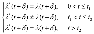
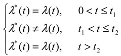
. This turns out to be a serious limitation for the present application: it implies that if X increases the saccadic pdf prior to t2, the pdf thereafter must be lower, just like the more efficient popcorn maker eventually makes less noise because most corn is already popped. Unfortunately, this violates the third condition in (2), where λ(t) = λ*(t) for t > t2; in other words, we cannot estimate the offset of the process X from the pdf. Another problem stems from the same constraint: because the pdf approaches zero for very long fixations, comparing the right tails of distributions becomes difficult (see Chechile, 2003; Luce, 1986; Van Zandt, 2000; Van Zandt & Ratcliff, 1995). For these reasons the pdf does not have the properties we sought in (2).
The hazard function, also known as the hazard rate, is a conditional index of intensity. It is defined as the pdf divided by the proportion of fixations that have not yet been terminated,
Jemr 03 00008 i005
where f(t) is the pdf and Jemr 03 00008 i015 
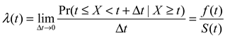
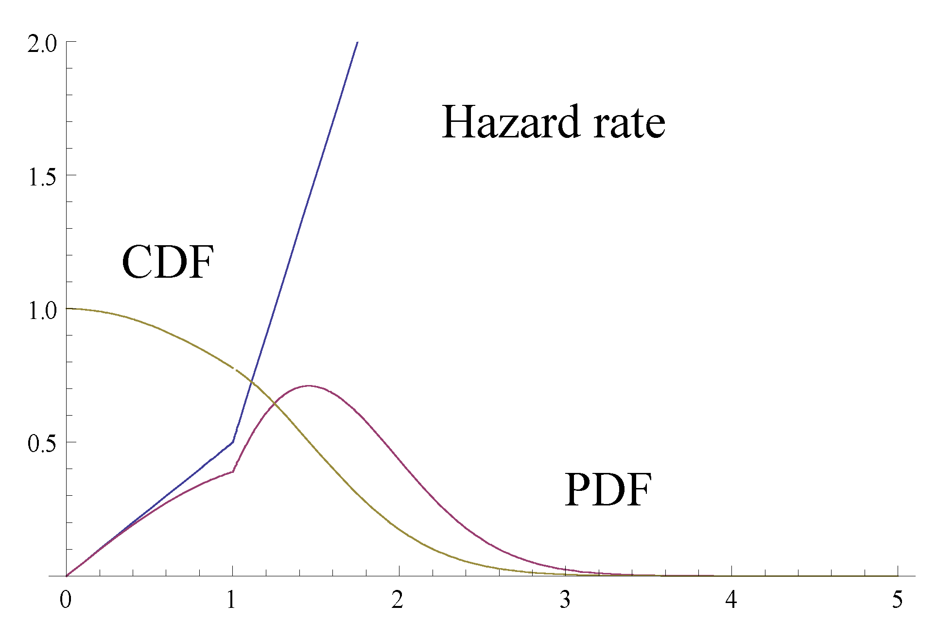
is the survival function of X. The hazard rate λ(t) can be seen as f(t) with its right tail magnified by a factor of 1/S(t). The two functions are closely connected:
Jemr 03 00008 i006
Nevertheless, there are important differences between them. Unlike the pdf, there are no inherent constraints on the shape of the hazard function, provided that Jemr 03 00008 i016 
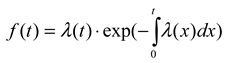
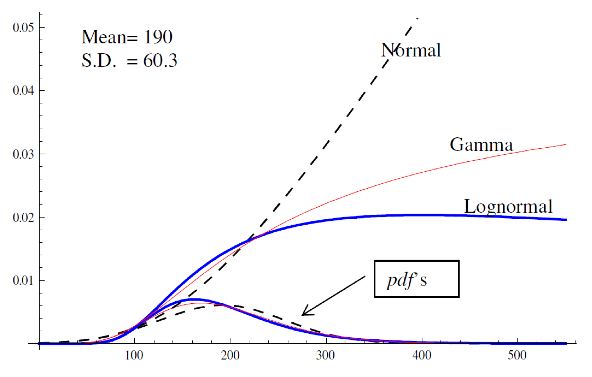
(i.e., the “lifetime” risk of saccade is infinity, to avoid “eternal fixations”). Figure 1 shows the pdf’s and hazard functions of three familiar distributions– the normal distribution, gamma distribution, and lognormal distribution – with the same means and standard deviations. All three distributions have been used as models of reading fixation duration (Feng, 2006; Reichle, Pollatsek, Fisher, & Rayner, 1998; Reilly & O’Regan, 1998). Despite similar shapes of the pdf’s, the hazard functions show distinct trajectories, especially at the right tail.
The hazard function λ(t) is an ideal candidate for (2). It measures the instantaneous risk of an event (e.g., a saccade) at time t, given that it has not yet occurred (Chechile, 2003; Hosmer & Lemeshow, 1999; Lawless, 1982). Thus the hazard function is conditionally independent from the history prior to t. This “memoryless” property of the hazard function satisfies (2): λ*(t) goes back to the baseline at t2 as soon as the effect of X goes away. The hazard function also allows us to compare the right tails of fixation duration distributions: it is easy to see that λ(t) ≥ f(t) because S(t) ≤ 1. The magnification is greater for longer fixations, as S(t) approaches zero.
Researchers of response time distributions have long recognized the advantages of the hazard function over the pdf (Chechile, 2003; Luce, 1986; Van Zandt, 2000; Van Zandt & Ratcliff, 1995). Its primary drawback is that it requires a large sample size, particularly for estimating the right tail. Fortunately, large eye movement corpora are not difficult to obtain, and some are publically available to researchers (e.g., Kennedy & Pynte, 2005).
An empirical example. Figure 2 shows a typical pdf (bottom curves) and the corresponding hazard function (top curves) of a reading fixation duration distribution. The data came from the Dundee Corpus (Kennedy & Pynte, 2005; Pynte & Kennedy, 2006), which includes over 400,000 fixations collected from 10 adult English readers reading newspaper stories. More details of the data and estimation methods can be found in the Methods section.
A number of observations are noteworthy in Figure 2. Numerically, the hazard function is always larger than the pdf, and the two functions become increasingly disassociated: whereas the pdf approaches zero after 300-400 msec, the hazard function remains substantially above zero and shows an unambiguous trend.
The hazard function in Figure 2 is a unimodal function, with a peak at approximately 250msec. It is also well captured by a piecewise linear regression model with three changepoints at approximately 130, 180, and 250msec. These parameters turn out to be common characteristics of most hazard functions examined in this paper. The second half of this paper investigates the shape and parameters of this function.
Finally, Figure 2 shows peculiar spikes every 41 or 42msec (or approximately 24Hz). The magnitude of the spikes is nearly twice of the expected hazard rate, suggesting a possible rounding artifact whereby fixations in nearby bins were combined. These artifacts must be removed, but the consequence of artifact removal differs for the pdf and the hazard function. With the pdf, simply removing the spikes would result in Jemr 03 00008 i017, because some probability mass is discarded. To ensure a proper pdf, one must re-norm the function, which will elevate the entire function (shown as the green line in Figure 2). In contrast, the hazard function is not subject to the same constraint. The piecewise linear regression in Figure 2 is estimated with artifacts simply removed. The less jagged black line is a smoothed version (using the 3RS3R algorithm; see Tukey, 1977) of the cleaned-up hazard rate, demonstrating the fit of the linear function.

Relation with Other Distributional Models

To summarize, the distribution of fixation duration carries rich information about underlying reading processes that can be recovered using the hazard function analysis. Here I focus on its relation with existing mathematical models of fixation duration distributions, and address other relevant issues in Discussion. It is important to remember, however, that diverse stochastic processes may result in the same distribution (e.g., Johnson, Kotz, & Balakrishnan, 1994). Thus a successful distributional model cannot identify the underlying mechanism. Nevertheless, it helps us narrow down the search for the true model, by rejecting processing models that make wrong distributional predictions.
Early attempts to model the pdf of fixation duration (Harris, Hainline, Abramov, Lemerise, & Camenzuli, 1988; Suppes, 1990; Suppes, 1994; Suppes, M. Cohen, R. Laddaga, Anliker, & Floyd, 1983) were met with limited success, in part because the choices of mathematical models were hardly informed by empirical distributions. More recently, Engbert and Kliegl (2001) proposed a semi-Markov model in which the hazard function for saccade generation varies with time. They nonetheless limited the hazard rate to a linear function (i.e., a Weibull distribution; see Johnson, et al., 1994), which is inconsistent with empirical data (see Figure 2).
A few recent models took advantage of empirical hazard functions. McConkie and colleagues (McConkie & Dyre, 2000; McConkie, Kerr, & Dyre, 1994) observed that the hazard function of reading fixation duration typically show three phases – a slow rising stage until approximately 100msec, and a fast rising stage to approximately 180msec, followed by a relatively flat tail. The three phrases could be modeled by a piecewise linear function. This motivated McConkie et al to derive a number of mathematical models, all of which fit an empirical distribution well. However, these models may not be able to account for the falling right tail of the hazard function observed in Figure 2, because they assume a serial processing model that includes a wait time distribution independent of other processes. Mathematically, this translates to a convolution of distributions with increasing hazard functions, which will always result in a rising hazard function (Barlow, Marshall, & Proschan, 1963; Marshall & Olkin, 2007). In search for a more flexible model, Feng (2006) reported that a mixture of three lognormal distributions can achieve good fit to diverse pdf’s of adult and child readers. Figure 1 and Figure 2 illustrate the qualitative similarity between the hazard function of the lognormal distribution and that of the empirical distribution. Both of these aforementioned models estimate the pdf, which becomes less informative as it approaches zero at the right tail. Few studies have directly modeled empirical hazard functions, with the noticeable exception of the Competition/Interaction theory (Yang, 2006; Yang & McConkie, 2001).
One of the most influential distributional models today, LATER (Linear Approach to Threshold with Ergodic Rate; Carpenter & Williams, 1995; Carpenter, 1999, 2000; Carpenter & McDonald, 2007; McDonald, Carpenter, & Shillcock, 2005; Reddi, Asrress, & Carpenter, 2003) conceptualizes saccade generation as a linear accumulation of information toward a fixed threshold. Assuming the speed of increase is normally distributed, the fixation duration follows a reci-normal distribution (Carpenter & Williams, 1995; Robert, 1991), which generally fits the cumulative distribution function of reading eye movements (Carpenter & McDonald, 2007; McDonald et al., 2005, with an additional component for short fixations). The reci-normal distribution is a special case of the generalized inverse normal distribution (see Johnson, et al., 1994; Robert, 1991). Except for some pathological cases, its hazard function is unimodal, with a fast rising phase followed by a slow descent, similar to Figure 2. Nonetheless, it appears that the reci-normal hazard function is not flexible enough to simultaneously account for both the fast rising and the slow falling phases of the empirical hazard function; it typically requires two functions to fit the whole distribution. Recent extensions of the LATER model (Moscoso Del Prado Martin, submitted; Nakahara, Nakamura, & Hikosaka, 2006) may help to improve its fit.
This brief survey underscores two observations. First, there is little consensus on how to infer the time course of cognitive processes from distribution functions. Second, more flexible mathematical tools are needed to capture the diversity in empirical distributions. The suggestion here is that the hazard function can serve as a bridge between empirical distribution functions and theoretical construes such as the time course of a cognitive process. Whether or not this particular proposal is successful, there is clearly a need for a more informative set of linking hypotheses.

The Empirical Study

The empirical part of the paper has two aims. The first is to illustrate the feasibility of the proposed hazard function analysis. More importantly, I will estimate ways in which the hazard function is influenced by a variety of reading-related factors, including language, age, and a number of processing variables. Since all of them have proven to have significant and differential influences on the mean fixation duration (Rayner, 1998), a straightforward hypothesis is that these diverse factors will show different time courses.
An accurate estimation of the hazard function, particularly at the right tail, requires a large sample of fixations. The present study includes large eye movement corpora from adult readers of four different languages (English, Chinese, Japanese, and Korean) and developing readers from two countries (US and China). Altogether more than one million eye movements were collected in four different labs around the world, using three different models of eye trackers. The size and the diversity of the data reduce the chance of random fluctuations and methodological artifacts.

Methods

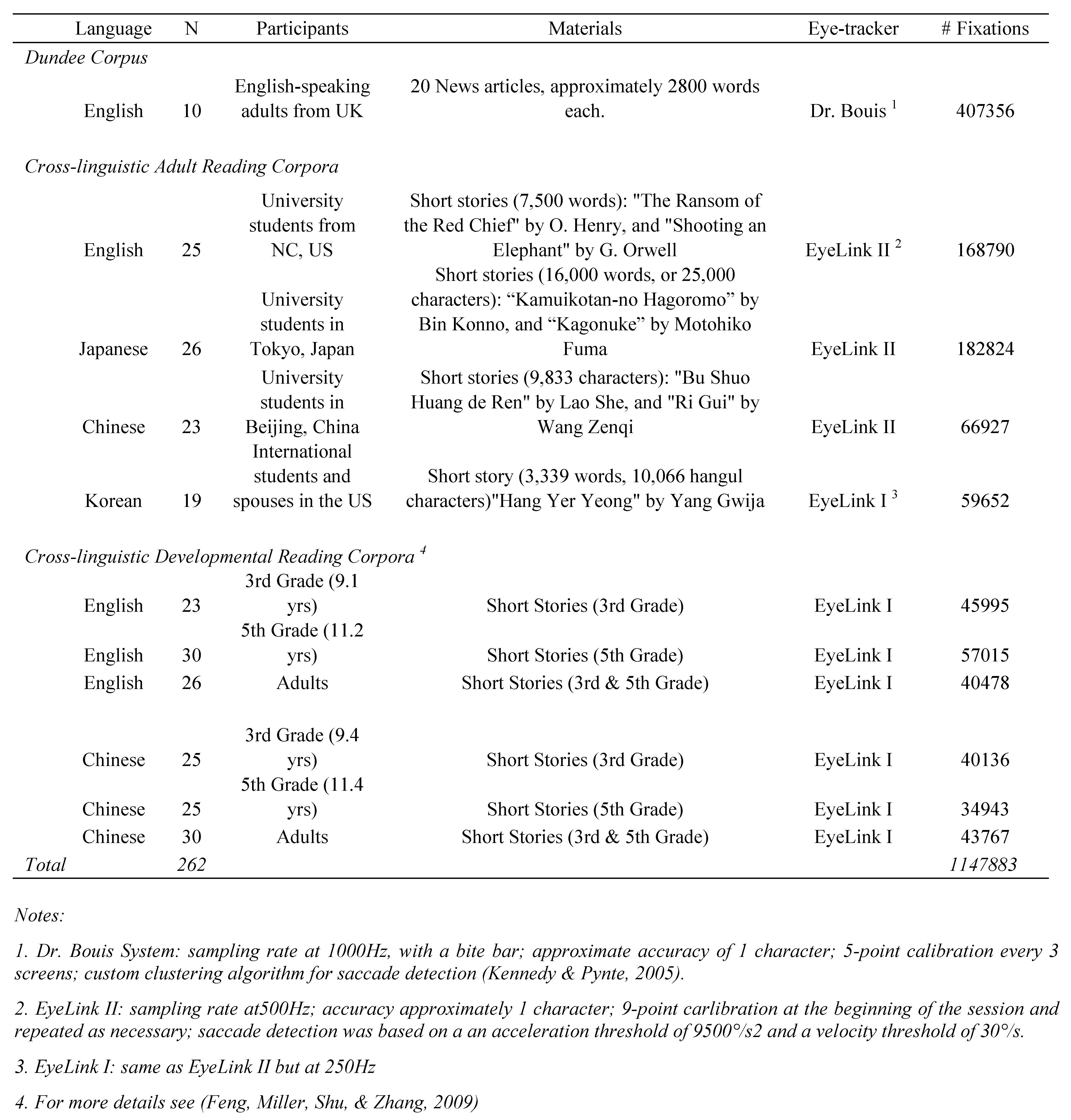
Corpora of Reading Eye Movements

The eye movement data used in this study came from 262 readers from three age groups and five countries. Data were collected in four different labs around the world using three different eye tracking systems. Table 1 summarizes key features of the databases. It is worth noting that there was no data censoring, i.e., no fixations were discarded because it is too short or too long. This is crucial for distributional analyses because the common practice of excluding long fixations – a form of right censoring (Le, 1997) – can dramatically inflate the hazard function.
The Dundee English Corpus. The Dundee corpus is a publicly available dataset that has been studied extensively by various research groups (Carpenter & McDonald, 2007; Kennedy & Pynte, 2005; Pynte & Kennedy, 2006). Eye movements were recorded using a Dr. Bouis system with a sampling rate of 1000 Hz. Fixations were detected using a custom-developed algorithm that clusters and merges samples of gaze locations into fixations (see Kennedy & Pynte, 2005). The algorithm differs from those in the EyeLink systems, and as we will see it may have caused some systematic differences in the rate of brief fixations. Further information about the corpus can be found in Kennedy and Pynte (2005; see also Pynte & Kennedy, 2006). I will focus on this dataset in a number of analyses because its size, quality, and availability.
Cross-linguistic Story Reading Studies. The cross- linguistic reading corpora include data from four languages: English, Chinese, Japanese, and Korean. Native-speaking adults were asked to read authentic novels in their own languages and answer multiple- choice questions after each story. Eye-movements were recorded with either the EyeLink I (the Korean study) or the EyeLink II (all other studies) eye tracking system, a head-mounted infrared system with typically accuracy of 0.5 visual degrees. A chin rest was used in conjunction with the built-in head movement compensation mechanism. Data from the right eye were used whenever available.
The studies also involved a gaze-contingent manipulation irrelevant to the present purpose. At the onset of every 8th-12th saccade, texts on the screen were shifted to the left or the right by approximately 1-3 character spaces. The shifts were designed to resemble naturally occurring oculomotor noises; effects of these screen shifts will be reported elsewhere. Here we focus on the majority of fixations that were not affected by the occasional screen shifts. Most of the screen shifts (94.5%) were imperceptible because the changes occurred during saccades or within 8msec after fixation onset; visual perception is suppressed during this period (Matin, 1974; Rayner, 1998; Wolverton & Zola, 1983). Fixations immediately after screen shifts were also excluded from analyses, even though they were not significantly affected by the manipulation. Approximately 4-12% fixations were excluded for these reasons for each reader.
Cross-linguistic Developmental Reading Studies. The next six sets of studies were designed to investigate developmental changes and orthographic effects in reading (Feng, et al., 2009). Participants were third- and fifth-grade students and adult readers in the US and China. They read two sets of short stories. One set included stories targeting the specific culture and reading level of the children. They were chosen from popular third- and fifth-grade extracurricular reading series published in each country. The other set, referred to as the “anchor stories,” included two stories with parallel versions in each language and allowed direct comparisons between languages. Feng et al. (2009) did not find significant differences between the two sets of stories, and data were pooled together in this paper.

Data Analysis

A series of analyses examine the effects of language, age, individual differences, word frequency, word length, and type of subsequent saccades. In each study, empirical hazard rates are estimated. Because most empirical hazard functions follow the same fast-rising-slow-falling profile, a flexible piecewise linear regression model is used to quantify the empirical curves. Key parameters such as the changepoints and slopes are then compared across conditions. Parameters of the piecewise regression model will be summarized in the final analysis.
Estimation of the hazard function. The hazard rate was estimated in one of two ways, depending on the sampling frequency of the data. When only the Dundee corpus (1000 Hz) was involved, the Kaplan-Meier product-limit estimator (Le, 1997) was used. The hazard rate and the standard error were estimated using the kphaz function in the muhaz package (v1.2.3; Hess & Gentleman, 2008) of the R language (v. 2.7.2; R Development Core Team, 2008). Due to their lower sampling rates, data recorded with EyeLink I (250 Hz) or II (500 Hz) systems were effectively grouped into 2 or 4msec bins, in which cases the actuarial method was more appropriate (Le, 1997). The SURVIVAL command in SPSS version 15.0 was used for this purpose. A 20msec bin width was chosen so that there were generally 30 or more “surviving” fixations in each bin. Following this procedure, the upper limit of the analysis was typically 400 to 600msec, depending on the size of the corpus.
A stable estimation of the empirical hazard function, particularly at the right tail, requires a large sample size. With exceptions of large corpora such as the Dundee Corpus, typical reading eye movement studies do not afford reliable individualized hazard rate estimates beyond three hundred milliseconds or so. Individual differences in the hazard rate will be examined with the Dundee database, whereas in other cases data are pooled across individuals. Using group data can potentially introduce biases, however (Ratcliff, 1979; Van Zandt, 2000). While this concern cannot be fully resolved in this study, there are reasons to believe the current approach is useful. Mathematically speaking, the pooled data are a mixture of individuals’ distributions. The hazard rate of the pooled distribution is a complex weighted average of hazard rates of individual distributions at a particular time. In principle, the right tail of the group hazard rate could be dominated by a few slow readers who have drastically different hazard rates from the rest of the group. The concern may be lessened, though not eliminated, by results reported below: readers in the Dundee corpus do not vary substantially in the hazard rate in the right tail; even 3rd grade students do not differ much from adult readers in the right tail of the hazard function. The robustness of the hazard function is interesting in itself – see Discussion – and it suggests the bias of group-data-based hazard rate estimation is likely to be small. This issue will be revisited in Discussion, and readers should keep potential problems of the procedure in mind.
Estimating changepoints. Prior research has shown that the empirical hazard function of reading fixation duration has a number of distinct phases and can be approximated by a piecewise linear function (McConkie & Dyre, 2000; Yang & McConkie, 2001). The segmented package for R (v 0.2-4; Muggeo, 2008) was used to fit a piecewise linear regression model to empirical hazard rates. Segmented differs from generic piecewise linear regression models in that it requires broken segments to be connected at changepoints (Muggeo, 2008). This constraint is important because we assume the underlying hazard rate of saccade generation is continuous.
The piecewise linear regression is only a heuristic tool for estimating the changepoints and slopes of empirical hazard functions, so that hazard rates can be compared across populations and conditions. It does not imply that the underlying biological mechanism has a linear hazard rate or goes through discrete phases during a fixation. Models based on continuous hazard functions provide more sophisticated explanations (e.g., Feng, 2006), though often at the cost of more assumptions about reading and oculomotor processes. A decision was made to stay closely to the data in this study and avoid unnecessary theoretical assumptions. For the purpose of comparing two empirical hazard functions, the segmented linear regression appears to be a straightforward descriptive tool. It is noteworthy, however, that a nonlinear model is required to capture a hazard function with a falling tail, because the falling linear regression line will eventually cross the x-axis and becomes negative. Nevertheless, the piecewise linear regression seems to suffice as a descriptive model for most of the analyses presented here.
It is currently not possible to automatically determine the optimal number of segments (Muggeo, 2008). The algorithm requires a manual specification the number of changepoints and initial guesses of where they are. Unless otherwise stated, the initial values were set to 100, 180, and 250msec (see Figure 2). Taking the initial values, the algorithm iteratively estimates the changepoints using a re-parameterized linear regression model (Muggeo, 2008). The solution depends more on the data than on the initial values, although occasionally the model can fail to converge due to poor initial specifications. The most common cause of failures to converge was that more changepoints were specified than the algorithm could find in the data. In this case the model was initialized to a 2-changepoint model (e.g., 100 and 250msec only).
Because the segmented regression model has not been used for empirical hazard functions, two Monte Carlo studies were conducted to illustrate statistical properties of this procedure. Appendix A examines the potential bias in estimating a changepoint in the hazard function. A piecewise-Weibull distribution was derived, which has a “segmented” linear hazard function with one known changepoint at 1.0. One thousand random samples of size 5000 were drawn from the distribution, and the “segmented” algorithm (Muggeo, 2008) was applied to estimate the changepoint. To be conservative, the Monte Carlo sample size 5,000 is smaller than samples used in the empirical studies. Based on the 1000 samples, the mean estimated changepoint is at 0.9970, with 95% confidence interval between 0.9317 and 1.0742. There is little evidence of bias in this example.
Appendix B investigates the potential bias of the reported SE. Ten thousand random samples of size 5000 were drawn (with replacement) from the dataset for Figure 7, which includes approximately 1,000,000 fixations by adult readers. For each sample, the hazard function was estimated and the segmented regression was performed with the initial changepoints set at 100, 180, and 250msec. The procedure was identical to that in the empirical studies. Data suggest that the SE estimation reported by the Segmented algorithm is biased, but it errs on the conservative side. That is, the true SE of the changepoint estimation is likely to be smaller than reported by the Segmented algorithm.

Results

The analyses to be reported fall into three groups. The first compares hazard functions among different readers, including (1) skilled readers of different languages, (2) children and adult readers, (3) individual readers reading the same materials. The second set of analyses explores how fixation duration is modulated by perceptual, cognitive, and other processing variables. To this end we will look at effects of (4) word frequency, (5) word length, and (6) types of subsequent saccades (forward, regression, or refixation). The final analyses will estimate the hazard function from all adult data and summarize estimated slopes and changepoints from previous steps.

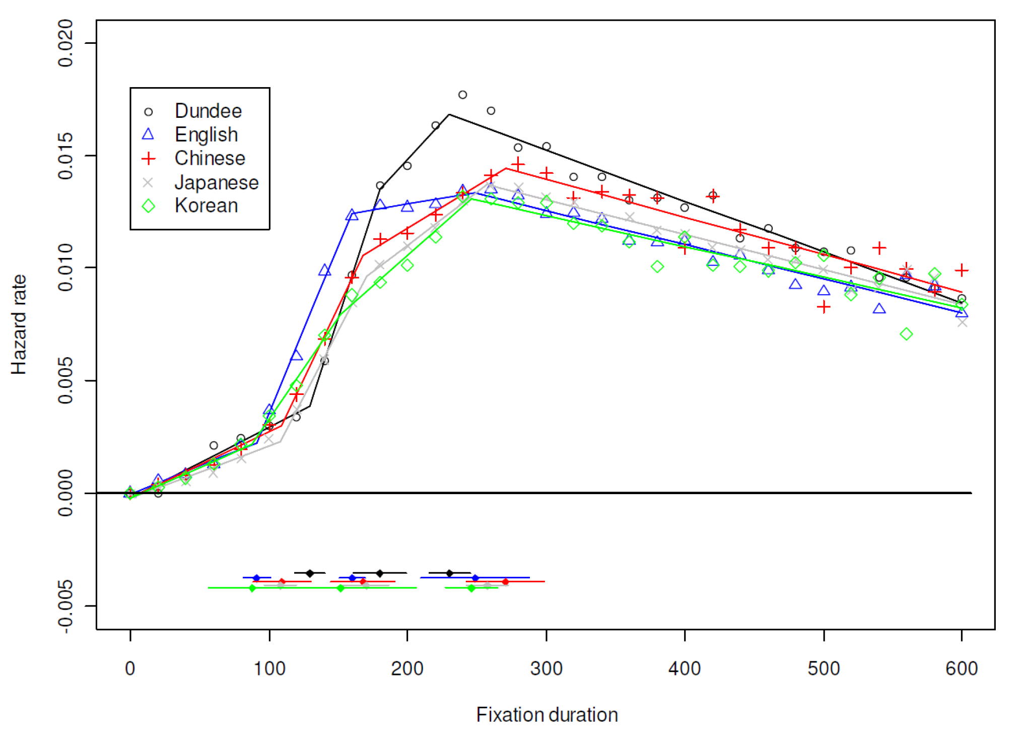
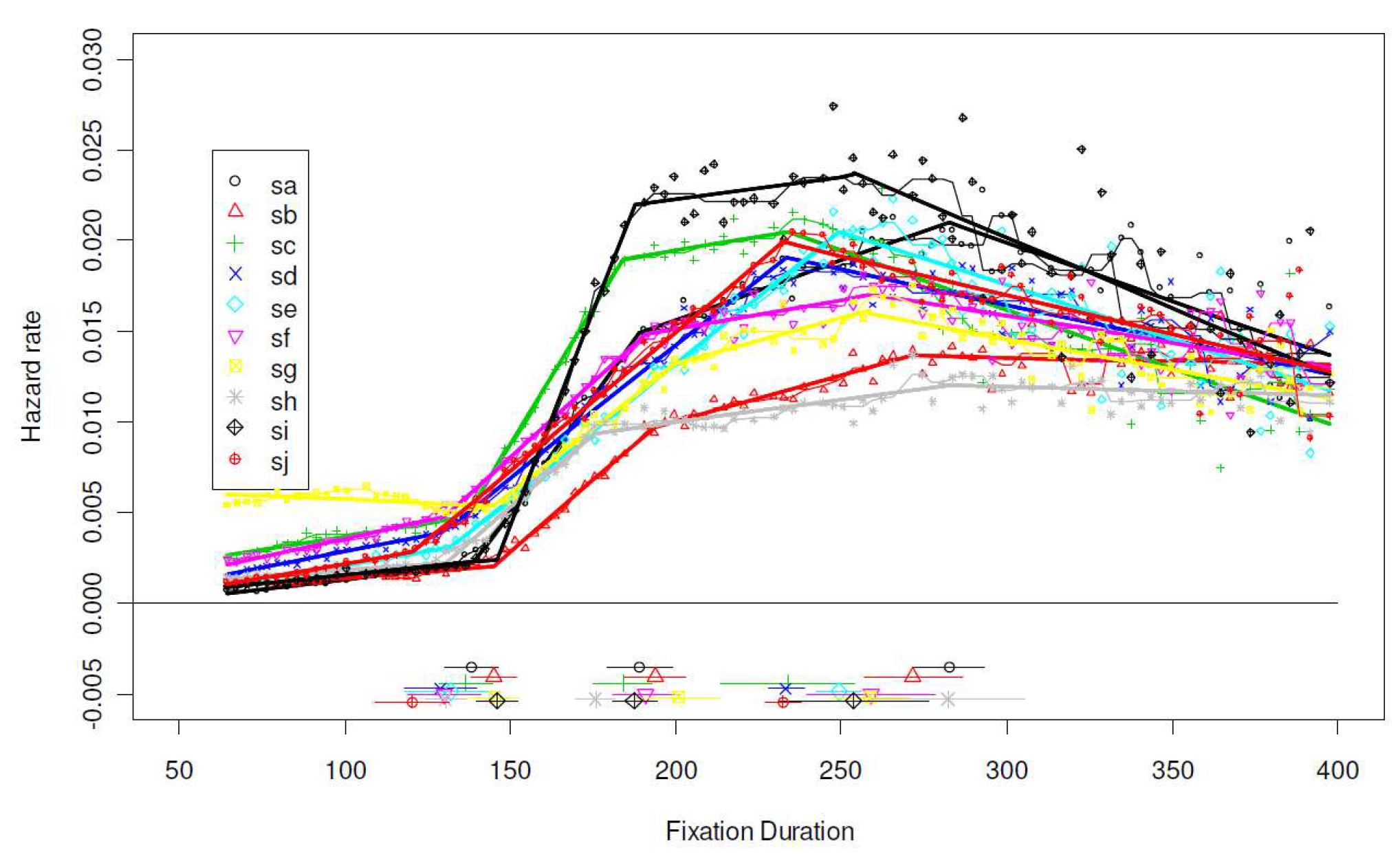
Language, Age, and Individual Differences

Language. The data for this analysis include the Dundee corpus and the cross-linguistic studies, involving adult speakers of English, Chinese, Japanese, and Korean reading authentic texts in their native languages. Hazard rates were estimated using the actuarial method based on 20msec bins and are shown in Figure 3. In addition, a piecewise linear regression analysis was conducted for each language using the segmented package for R (Muggeo, 2008); see Figure 3. The line segments near the bottom of the figure mark the 95% confidence interval of the estimated changepoints, centered at the estimated values (the dots).
The hazard functions follow a stereotyped time course: it rises to a peak at approximately 250msec, and then gradually falls. Compared to the near linear decrease, the slope of the rising curve is uneven. It rises slowly before approximately 100msec. Between 100msec and 180msec, the rate increases drastically. From 180msec, the hazard function rises at a slower speed until reaching its peak near 250msec. The locations of estimated changepoints are consistent across languages. In most cases the estimates are within confidence intervals of each other, with the exception of the first changepoint of the Dundee data. This is likely due to differences in saccade detection algorithms in different eye trackers.
Despite the stable timing of the changepoints, the hazard function varies by language. There is relatively little language difference in the initial phase (before 100msec) or in the decline phase (after approximately 250 ms). Differences emerge during the short time window between approximately 100 and 180msec. The two English datasets show similarly steep slopes, compared to the three East Asian languages. Interestingly, by the time when most hazard functions take a downturn at around 250msec, the hazard rates of all studies have converged to close to 0.015.
Age/reading expertise. Figure 4 compares 3rd- and 5th- grade children and adult readers from the US and China, reading authentic children’s stories in their own languages. Despite the ease of reading materials, adults’ hazard functions are similar to those in Figure 3. Hazard functions of developing readers also show three distinctive stages. This is confirmed by the segmented regression analysis. Estimated changepoints are consistent across ages and languages. The pivotal points are, again, approximately 100, 180, and 250msec.
Developmental differences are equally salient. Compared to adults, children have lower hazard rate before 100msec, although there does not appear to be a difference between 3rd- and 5th-grade students in either country. However, the three age groups diverge between 100 and 250msec, where after 180msec hazard functions of adult readers continue to increase but those of children are virtually flat. After 250msec, hazard rates for children decrease at a much slower pace than those of adults. Having lower hazard rate in the right tail means children make more long fixations than adults, a finding consistent with Feng (2006).
Individual differences. Using group data in distributional analyses raises two concerns. Individual readers may have idiosyncratic distributions that may be masked in group analyses. In addition, the group distribution could be dominated by slow readers because they make more fixations. To address these concerns, Figure 5 shows estimated hazard functions of all 10 readers in the Dundee corpus. Each reader made between 29,000 and 47,000 fixations. The mean fixation duration ranges from 173 to 230msec. For all readers the initial parameters for the piecewise regression were set to 100, 180, and 250msec. The segmented algorithm failed to converge for 3 readers (sd, se, and sj), because it could not detect a changepoint at around 180msec. Indeed these readers’ data suggest a linear increase from 100 to 250msec. In these cases their regression lines were based on initial values of 100 and 250msec. The thick straight line segments represent the estimated piecewise regressions, and the thin jagged lines are smoothed (using the 3RS3R algorithm; see Tukey, 1977) empirical hazard rates.
The timing of changepoints is largely consistent across readers, at approximately 130, 180, and 250msec. Without exceptions, the hazard function begins with a slow rising phase, followed by a fast rising phase between 130 and 250msec, and a slow decline phase afterwards. Most readers also show a deceleration of the hazard function between 180 and 250msec. The first changepoint is 30msec later than estimates from other datasets; this is likely attributable to how different eye trackers handle brief fixations. Estimates of the changepoint at around 250msec tend to have large confidence intervals, reflecting increased noise levels in the right tail.
Individual differences exist in all phases of the hazard function. For example reader se made a large number of express saccades (shorter than 130msec), but otherwise showed a typical hazard function. Reader si had virtually no express saccades but the steepest rise between 130 and 180msec, and therefore had the shortest average fixation duration overall. Readers sb and sh, on the other hand, show hazard functions resembling those of children in Figure 4. Nonetheless, the differences are mostly in the rate of changes in the hazard function, not when changes happen. Another important finding is that individuals’ hazard functions tend to converge toward the right tail. At around 400msec the hazard rates are generally between 0.010 and 0.015, consistent with the estimate from the pooled data (see Figure 3).

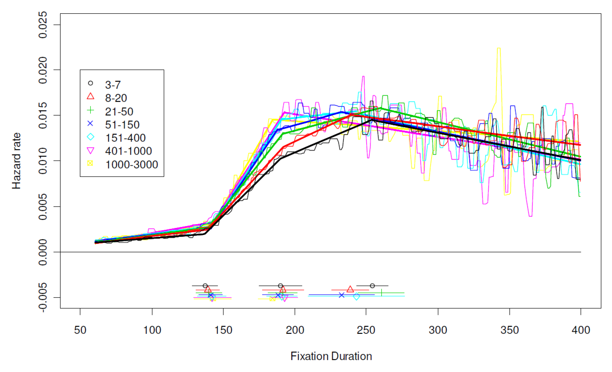
Modulation of Hazard Function by Processing Variables

The next three analyses focus on variables that are known to influence moment-to-moment reading processes. They are based on the Dundee corpus, which has the largest sample size among all corpora.
Word frequency. The Dundee corpus includes as a variable the frequency of occurrence of each word in its text base. The frequency was discretized into eight classes according to the natural logarithm of the frequency. Only words that occurred between 3 to 3,000 times were included in this analysis; very rare words and extremely frequent words (such as “the” and “of”) were excluded. In addition, to lessen the correlation between word frequency and word length, the data were further constrained to only words 4 to 7 letters long. Only the first fixation on a word was used in this analysis. The sample size varied across frequency categories, ranging from over 49,000 fixations (frequency 8-20) to 4884 fixations (for frequency 1000-3000). As expected, the mean fixation duration show a linear decrease from 202msec in the lowest frequency category to 189msec in the highest frequency category. The focus of this analysis, however, is on distributional properties that underlie the frequency effect.
Figure 6 shows the estimated hazard function for each frequency category. When the initial values of changepoints were set to 100, 180, and 250msec., the segmented regression failed to converge for the two highest frequency categories because of the lack of a changepoint around 250msec. Instead, initial values 100 and 180msec were used for these two categories. The thick lines on Figure 6 represent estimates of piecewise linear regressions, whereas the corresponding jagged lines are empirical hazard rates, smoothed using the 3RS3R algorithm (Tukey, 1977).
Across the board, there is no evidence that the timing of the changepoints is systematically influenced by word frequency. On the other hand, word frequency has a strong impact on the hazard function of fixation duration, though its effect is limited to the slope of the fast rising phase. Familiar words results in fast rising hazard functions between 140 and 190msec, and the differences remains until approximately 250msec. The largest effect of word frequency is observed at about 190msec. Outside the window between 140 and 250msec, word frequency appears to have little effect on saccade generation. In particular, if a fixation on a low frequency word is not terminated by 250msec, its risk of it being terminated is the same as a fixation on a high frequency word.
Word length. The length of a word may be perceived during the preceding fixation, and therefore it may potentially have a different time course from that of word frequency. Figure 7 shows hazard functions of the first fixations on words between 3 and 8 letters long. There were between approximately 34,000 and 62,000 first fixations in each word length category. The mean first fixation duration ranged from 191msec (3-letter-long words) to 202msec (8-letter-long words). The estimated changepoints are generally consistent across word lengths, and are comparable to those in previous analyses. Similar to that of word frequency, the effect of word length is again limited to the fast rising phase between 140 and 250msec, with the strongest effect at approximately 190msec. Word length appears to share a similar time course as word frequency.
Type of subsequent saccades. Refixations and regressions are sometimes assumed to be triggered by different mechanisms from forward saccades (e.g., Reichle, et al., 2006). In this analysis, fixations are classified into three categories based on the target of the subsequent eye movements – forward (to a word down the line), regression (to a previous word), and refixation (to the same word). The respective sample sizes were 305,334, 67,564, and 27,925 and the mean fixation durations were 203, 175, and 187msec. The estimation was the same as previous analyses, with the standard initial parameters of 100, 180, and 250msec.
The estimated hazard functions are shown in Figure 8. Due to smaller sample sizes, the hazard rate estimates for refixations and regressions are noisier, and the corresponding confidence intervals for changepoints are larger than those of forward fixations. Nonetheless, locations of the first two changepoints are again consistent with previous values, and do not differ substantially by types of saccades. The third changepoint appears to be later for refixation and regressions compared to forward eye movements, but this observation needs to be interpreted with caution given the large confidence intervals.
Despite similarities in the timing of the changepoints, the hazard functions for different types of fixations differ markedly. Unlike previous analyses, hazard functions diverge in the initial slow rising phase, where refixations and regressions are triggered at rates more than double that of forward saccades. The largest difference among the three conditions appears at the first changepoint, at approximately 140msec. The higher saccade rates for refixations and regressions remain until approximately 180msec, after which point they are surpassed by forward saccades. Refixations also differ from regressions in that by the third changepoint (about 280msec) the hazard rate for refixation is substantially lower than that of regressions. A higher initial hazard rate means excessive short fixations, whereas a low hazard rate leaves a relatively heavy right tail in the pdf. The net result, though, is an overall shorter average fixation. Subtle distributional differences like these can not be recovered by comparing the means.

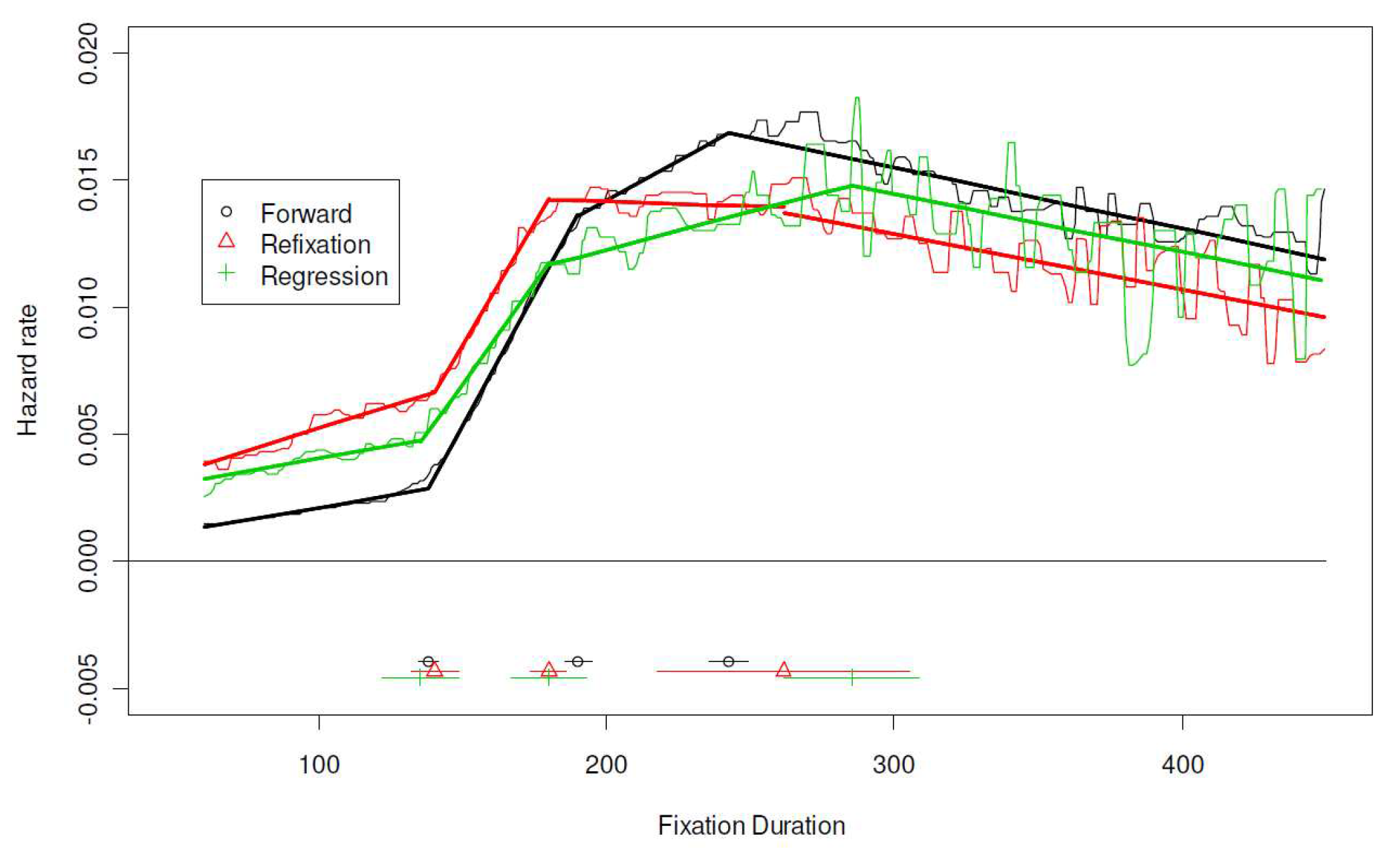
Pooled Hazard Functions

Although the segmented linear regression is a useful descriptive tool, the hazard function cannot decrease at a linear rate forever because it would at some point become negative. Eventually the hazard function will curve as it approaches its asymptote at 0. A large sample is needed to demonstrate this. Fortunately, Figure 3 and Figure 4 suggest that there is little language difference in the right tail of the hazard function. Thus, data from all 164 adult readers were pooled together in this analysis, which yielded over one million fixations. Similarly, English- and Chinese- speaking children’s data were combined within each age level, which resulted in over 110,000 fixations per age group. These combined datasets allow relatively robust estimations of the hazard function at up to 2000msec.
Figure 9 shows estimated hazard rates for all 3rd- and 5th-grade students and adult readers. Estimated hazard rates are marked with solid dots, and the corresponding standard errors are shown in vertical bars. The bold curves, a smoothed version of the hazard functions, are constructed using a simple moving average technique (no smoothing between 0 to 400msec, 3-sample averages between 400-600msec, 5-sample averages between 600 and 1000msec, and 7-sample windows thereafter). Although other estimation techniques exist (Le, 1997; Luce, 1986), this simple method works well for the present purpose. The thin lines represent the corresponding pdf’s of fixation duration. Three vertical lines mark the three recurring changepoints at100, 180, and 250msec.
As predicted, the rate of decline gradually decelerates for all three hazard functions. Overall, Figure 9 suggests that the hazard function of reading fixation duration involves four phases – (a) 0-100mse, slow rising, (b) 100- 180msec, fast rising, (c) 180-250msec, decelerated rising, and (d) >250msec, slow decaying. Although the first three phases can be approximated with segmented linear functions, the last phase will ultimately require a non- linear function.
Figure 9 also shows how the pdf’s are related to the hazard functions. Coincidentally, all pdf’s peak at 180msec, where the rise of the hazard functions abruptly slows down. The reason for this deceleration is unknown. Moreover, there appears to be a “bump” at approximately 250msec in all pdf’s, which corresponds to the dramatic turn of the hazard function at the same time.

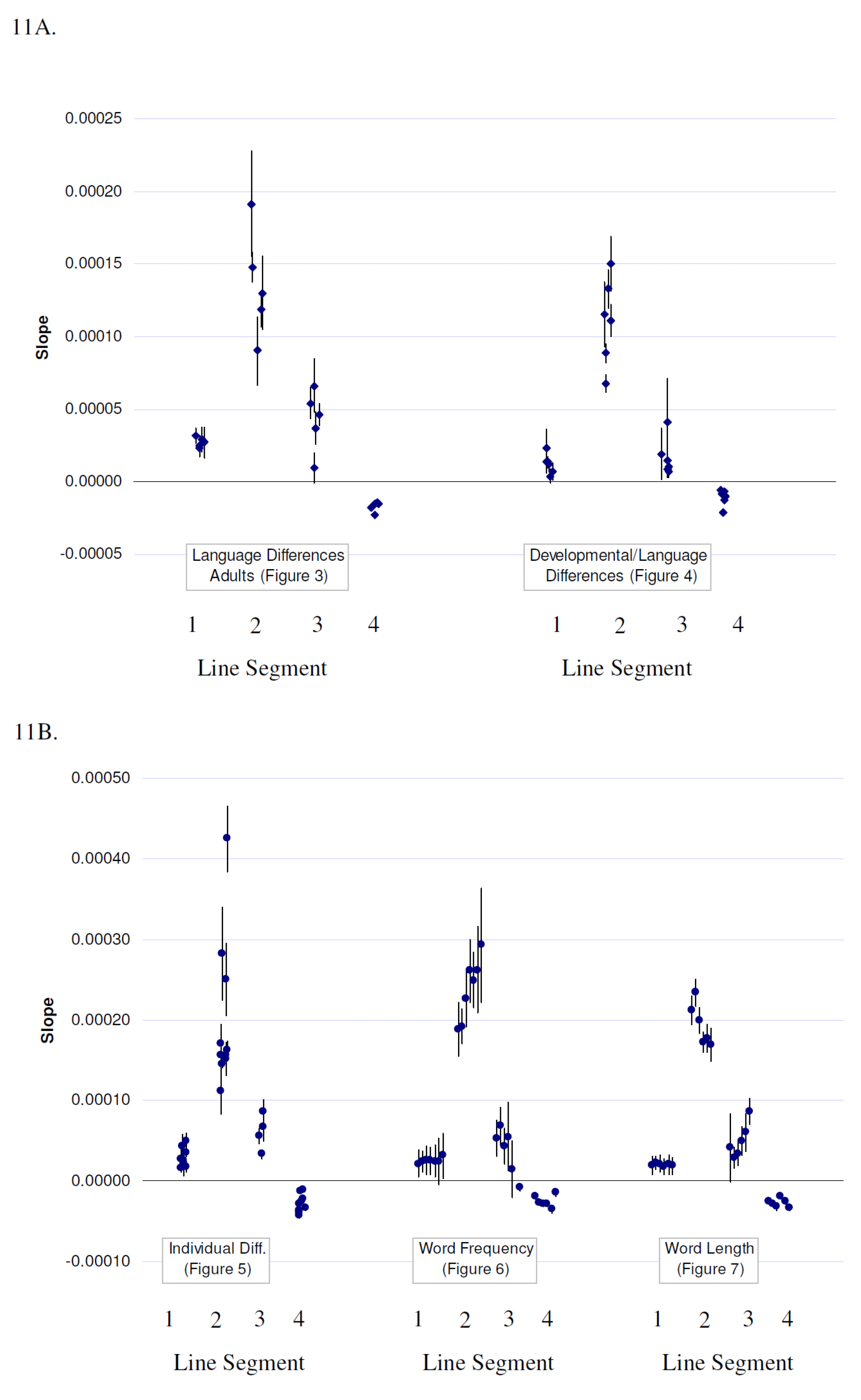
Summary of Changepoints and Regression Slopes

Figure 10 and Figure 11 summarize the changepoints and slopes from Figure 3, Figure 4, Figure 5, Figure 6 and Figure 7. Figure 10A plots the estimated locations of changepoints from 11 independent samples (see Figure 3 and Figure 4); data are jittered for clarity. The error bars represent standard errors of estimation, reported by the segmented algorithm. The 3-changepoint model provides excellent fit to the data, and the estimated locations of changepoints are consistent across studies.
The first changepoint is at approximately 100msec, though the Dundee corpus always comes out higher. The second changepoint is consistently between 150 and 180msec, averaging about 170msec. The last changepoint shows more variability because hazard rate estimates are much noisier in the tails. But nonetheless the values consistently center around 250msec. Figure 10B shows effects of individual differences, word frequency, and word length (see Figure 5, Figure 6 and Figure 7), all of which are based on the Dundee corpus. Despite individual differences, estimates cluster together, with no overlap across changepoints. Moreover, the estimated changepoints are not associated with word frequency or word length.
The same cannot be said for the slope parameter. Figure 11A,B illustrate the magnitude of the slope for each segment in previous figures. Error bars represent standard errors of the slope parameters. Figure 11A shows substantial variation in the second and third slopes, i.e., slopes between 100 and 180msec and between 180 and 250msec. Figure 11B clearly demonstrates that as word frequency increases, the slope of the 2nd segment (the fast rising phase between 100-180msec) increases correspondingly. Similarly, the slope decreases as words become longer. There is also an interesting negative correlation (r= -0.80 and -0.55 for word length and word frequency analyses, respectively) between slopes for the 2nd segment and the 3rd segment (between 180 and 250msec). The reason for this negative relationship is unknown, but the net result is that the peak hazard rate at 250msec is kept in the neighborhood of 0.015 to 0.020.
Not all slopes are subject to systematic influences, though. The slope between 0 to 100msec is low but consistent across datasets, so are the negative slopes of the declining phase after 250msec. These stable slopes, along with the consistent timing of the changepoints, strongly constrain the overall shape of the hazard function of reading fixation duration.

Discussion

The present paper was motivated by the lack of a general linking hypothesis that allows a direct estimation of the time course of reading processes from empirical fixation duration data. I argue that this goal is unattainable within the traditional linear statistical framework. A set of new linking hypothesis is developed based on the assumption that a change in a reading process should affect the intensity of eye movements in real-time. This leads to a focus on the empirical hazard function of fixation duration distributions. Using this logic, the present study confirms a stereotypical hazard function of reading fixations (see Figure 9) that is generally consistent with previous reports (Feng, 2006; McConkie & Dyre, 2000; McConkie, et al., 1994; Yang, 2006; Yang & McConkie, 2001). In addition, I illustrated how reading eye movements are influenced by various processing and individual differences variables, but in ways that are not predicted by current theories. I will discuss the logic for the model and its implications for theories of reading eye movements.

Linking Distributions to Processes: The Instantaneity Assumption

A key to the current model is the assumption that the effect of a reading process is reflected immediately on the hazard function (see next section about the oculomotor delay). This does not imply that a change in a reading process deterministically triggers a saccade; rather, the immediate impact is on the instantaneous likelihood of a saccade. The instantaneity assumption is consistent with contemporary models of reading eye movements, such as SWIFT (Engbert, et al., 2005; Richter, Engbert, & Kliegl, 2006) and the Competition/Interaction model (Yang, 2006), in which reading processes modulates the probability of saccades in real time.
The instantaneity assumption is nevertheless not compatible with models where there is no consistent temporal mapping between reading processes and saccadic events. This happens in a strictly serial model, where a reading process X has no effect on the fixation duration until a subsequent random process Y is completed. In this case the fixation duration involves the sum of the two processing delays. Mathematically, the distribution of the sum of two random variables is the convolution of the two component distributions. Convolution, of which the moving-average is an example, scrambles temporal information about X with that of Y. When the variance of Y is small, the scrambling or jittering is localized. But with large variance in Y, signals of X are diffused over a wide time window, potentially the entire distribution of fixation duration, in which case recovering the time course of X is difficult.
In short, the instantaneity assumption is a powerful assumption and should not be made lightly. But if deemed appropriate, it promises a pathway to recovering the time course of reading processes from the distribution of fixation duration. Even when the assumption does not hold strictly, the consequence may be moderate and tolerable when the intervening random variable is small. More sophisticated models may be developed to deal with independent noises, for example, through deconvolution.
The oculomotor delay. In this paper, δ represents the hypothetical “dead time” in which reading processes have no influence on saccadic decisions. Importantly, it is not the time to “program” an eye movement: the present model does not assume independence between oculomotor programming and high-level reading processes. As long as saccadic programming is open to the moderation by reading processes, the effect will be reflected on the hazard function and therefore is not part of δ. In the derivation of the present model, δ is assumed a constant, which is obviously an idealization. It is likely to be a random variable, but its mean and variance are expected to be small (e.g., Cutsuridis, Smyrnis, Evdokimidis, & Perantonis, 2007, used 20msec as an estimate of the time from burst neurons to eye muscles) and thus unlikely to be a serious threat to the instantaneity assumption. Future research is need to investigate this effect.

Toward a Model of Reading Eye Movement Control

The paper began with a generic linking hypothesis (2) between the hazard function of fixation duration and the time course of a reading process. Empirical data from large eye movement corpora uncovered additional regularizes in the data that allow further refinements of the theoretical model. Two observations stand out: the robustness of the hazard function and the way in which higher-order processes influence the fixation duration distribution. I will recap these results before presenting a revised model and discuss its implications.
Fixed time course, flexible slopes. Perhaps the most unexpected finding of this study is the consistent timing of the changepoints of hazard functions. This is not attributable to the linking hypothesis – it does not restrict the shape of the hazard function. Given the large sample sizes and diverse datasets involved in this study, these findings are unlikely to be due to chance or statistical artifacts. On the other hand, the hazard rate of reading fixation duration is systematically influenced by inter- and intro-individual variables. As shown in Figure 11A and Figure 11B, the modulation effect concentrates on two specific parameters, namely the slopes during the fast- rising phase of the hazard function, between 100- 180msec and 180-250msec. It is also interesting that the hazard rate remains a piecewise-linear function during these time windows, which implies that the modulation effect is sustained and near constant between critical changepoints.
The interesting question is what caused these changes in the saccadic rate. Traditionally, reading eye movements are thought to be triggered by events outside of the oculomotor system, for example by the completion of certain stage of lexical processing (e.g., Morrison, 1984; Reichle, et al., 1998). According to this model, the locations of changepoints should depend on the distribution of lexical processing time, e.g., earlier for familiar words and later for low frequency words. This is no what was observed (see Figure 6). Moreover, one would expect different changepoints for beginning and skilled readers because children take more time to recognize words (McConkie, et al., 1991; Rayner, 1986). This is again not the case (Figure 4). None of the factors examined here – language, age, individual differences, word frequency, word length, or the previous saccade – seems to systematically influence the changepoints of the hazard function. Future studies should, for example, investigate the effect of word frequency for each individual reading at each word length. But given the robustness of the changepoints shown here, we cannot ignore the possibility that the basic shape of the hazard function, including the changepoints, is characteristic of the oculomotor system rather than the exogenous factors examined here.
Under this backdrop, it is interesting to consider how high-level reading processes modulate and control reading eye movements. In the final section I will outline an extension of the segmented regression model that incorporates empirical constraints observed in this study. The model is intentionally inductive and restrictive, which complements more sophisticated modeling approaches (Feng, 2003, 2006, 2009). It makes falsifiable predictions about how the saccadic rate is modulated by reading processes that can be easily tested in future research.
A Proportional-Hazard model. An interesting consequence of having segmented linear regressions with fixed changepoints is that cognitive/linguistic effects may be estimated using the proportional hazard model (Cox, 1972; Martinussen & Scheike, 2006).
Using the notion of (2), let λ(t) be the baseline hazard function for reading fixation duration and λ*(t) be the hazard function under the influence of a process X. In the present study λ(t) is well approximated by a 3- changepoint segmented linear regression λ(t) = bit + Ci, where bi and Ci are the slopes and intercepts for the four linear functions defined by the three changepoints t1, t2, and t3; the timing of the changepoints is constant, at approximately 100, 180, and 250msec, and is independent of all the factors examined here. On a whole, the present study suggests that the risk of saccade under X is proportional to that in the baseline condition
Jemr 03 00008 i007
where pi (i ∈[1,4]) are constant relative risks for the four phases. Obviously, pi > 1 when X increases the hazard function during this period, and vise versa.
Moreover, Figure 11 suggests that (6) can be further constrained: with a few exceptions, p1 = 1 and p4 = 1, i.e., high-level processes do not modulate the hazard function during the initial slow rising period or the final slow decline period. Also, it is reasonable to assume C1 = 0, and thanks to constraints of the segmented regression model, other Ci are determined by the endpoint of the previous segment and are not free parameters. Thus, for most higher-order reading processes, their effects on the intensity of saccades can be characterized by
Jemr 03 00008 i008
The model (7) is restricted: given a baseline hazard function λ(t) = bit + Ci, there are only two free parameters, p2 and p3, to be estimated. Developing statistical tests for ti and pi is beyond the scope of the present paper, but since (7) is a straightforward extension of the proportional hazards model in survival analysis (Cox, 1972), similar techniques in survival analyses can be used here (see Martinussen & Scheike, 2006). Additionally, the pdf and moments (e.g., the mean and variance) of the fixation duration distribution can be derived – symbolically or numerically – using (5). In theory the last segment (t > t3) must be replaced by a nonlinear function in order to be a valid hazard function, but the notion of a proportional hazard model is equally applicable.
On the Underlying Mechanism. What does the proportional-hazard model (7) tell us about the underlying psychological and neurophysiological processes? To this end we note that (7) depicts the evolution of the hazard function over time:
Jemr 03 00008 i009
where a(t) is a step function that changes values at the pre-defined changepoints ti. Alternatively, if we assume time is discrete rather than continuous, we have
Jemr 03 00008 i010
In words, the risk of making a saccade at one moment is the sum of the risk at the previous moment and a moderation term that is mostly constant except changes at critical times. This suggests a very simple control mechanism, whereby reading eye movements are generated by a random process, where its key parameter, the moment-to-moment saccadic risk (i.e., the hazard rate), is moderated by the activation level a(t) of an input node, A, for lack of a better name. Note that up to this point the mechanism is general enough to describe virtually any hazard function, but findings from this study reveal some peculiar properties of A.
First, the empirical hazard function, as depicted by (7) or (9), is simple enough to suggest that A acts as the main conduit between the random saccade generation process and other processes. A potential candidate is the superior colliculus, which hosts the fixate and move centers and is connected to a wide network of brain regions (Carpenter, 2000; Findlay & Walker, 1999; Munoz, 2002). While the superior colliculus is not the sole source of saccadic commands, it may be the primary channel of control during natural reading.
Second, the temporal profile of A is also interesting: its activation level is a step function, jumping between stable states. If node A is kicked into different gears by input from various brain regions, then the present model predicts that these control signals arrive at relatively fixed delays after the onset of a fixation. Supportive evidence comes from Yang and McConkie (2001), who found the saccade hazard rate was strongly inhibited between 125-175msec when texts were masked by non-text like stimuli such as unspaced X-strings and blank pages, and between 175-250msec in conditions where words were replaced with nonwords. This suggests the phase changes at 120msec and 180msec are triggered by input from perceptual and lexical processes, respectively. Hints also come from the current study. For example, the peak of word frequency effect is also at around 190msec; developmentally, children’s hazard functions become flat between 180-250msec, which could be associated with the lack of automaticity in word recognition. In addition, saccades are mostly suppressed prior to 100msec, except when voluntary saccadic strategies such as regressions or refixations are to be carried out, in which cases the hazard rate is substantially raised. The idea that signals from different processes arrive by a fixed schedule requires further research.
Finally, the model (9) implies that effects of higher- order reading processes are also mediated by A, because both pi and bi are bound by the same time windows defined by the changepoints of the hazard function. Data also suggest that the modulation is generally small and relatively brief during normal reading. Nonetheless, such moderate moderation is more than enough to generate reliable differences in mean fixation durations and in distribution functions.
The hazard function model presented here is first and foremost a descriptive model for the distribution of reading eye movements. The segmented linear regression is arguably the simplest tool to capture these changes, but it needs not to imply that the underlying mechanism is discontinuous or linear. The important message is that the empirical hazard function takes predictable turns at predictable times. So far no mechanistic model of reading eye movements can fully explain the timing and directions of these changes. A statistical model of eye movements, no matter how precise, cannot positively identify the underlying stochastic mechanism without additional processing assumptions. The linking hypothesis and the processing model outlined above is a step toward this direction.

Funding

This research is supported in part by NIH grant 5R03HD051909-02. The author wishes to thank Dr. Alan Kennedy for sharing the Dundee corpus. Drs. Nobuyuki Jincho, Yoonhyoung Lee, Eike Richter, Reiko Mazuka, Eric Reichle, Ralf Engbert, Dirk Vorberg, and an anonymous reviewer provided helpful comments on early drafts. Address correspondence to: Gary Feng, Department of Psychology & Neuroscience, Box 90085, Duke University, Durham, NC 27708. (email: garyfeng@duke.edu).

Appendix A. A Monte Carlo Study of Potential Biases of the Segmented Algorithm

Segmented (Muggeo, 2008) is a general purpose regression model and has not been applied to estimating changepoints in the hazard function. This study examines its ability to recover changepoints from a distribution with segmented linear hazard functions.
We begin by specifying a two-piece segmented linear function as the hazard rate model.
Jemr 03 00008 i011
where d is the location of the changepoint, and a and b are parameters controlling the slopes. Using (5), the corresponding probability density function is
Jemr 03 00008 i012
which is a piecewise Weibull distribution (Johnson, et al., 1994). See Figure A1. Its cumulative distribution function (CDF) is
Jemr 03 00008 i013
A random sample can be generated from this distribution by first generating a uniform random number between 0 and 1, and plug it in the inverse function of the CDF.
Figure A1. The hazard function, PDF, and CDF of the piecewise Weibull distribution used in Appendix A.
Jemr 03 00008 g0a1
The Monte Carlo study was done in R (v2.7), and the source code is available upon request. In this example we set a = 0.5, b = 1, and d = 1. As a result, the slope of the first segment is ¼ of the slope of the second segment, similar to what is observed in the empirical data. A total of 1000 Monte Carlo samples were drawn, each of which included 5000 random numbers generated from the aforementioned distribution. With each Monte Carlo sample, the hazard rate was first estimated using the kphaz routine, with a bin size of 0.01. The segmented routine was then employed to estimate the changepoint in the hazard function. We initialized the model to a single random changepoint between 0.75 and 1.25. This procedure was repeated 1000 times.
The frequency distribution of the estimated location of the changepoint is shown in Figure A2. The distribution appears to be symmetrical around d = 1. Indeed, the mean estimated changepoint is at 0.9970, with 95% confidence interval between 0.9317 and 1.0742. Based on this example, there is little evidence for biases in the procedure used to estimate the empirical hazard function and to estimate the changepoint. Although this far from a systematic examination of the algorithm, which is beyond the scope of the current paper, the current example adds to the confidence in the methodology.
Figure A2. The distribution of estimated changepoint based on 1000 Monte Carlo samples.
Jemr 03 00008 g0a2

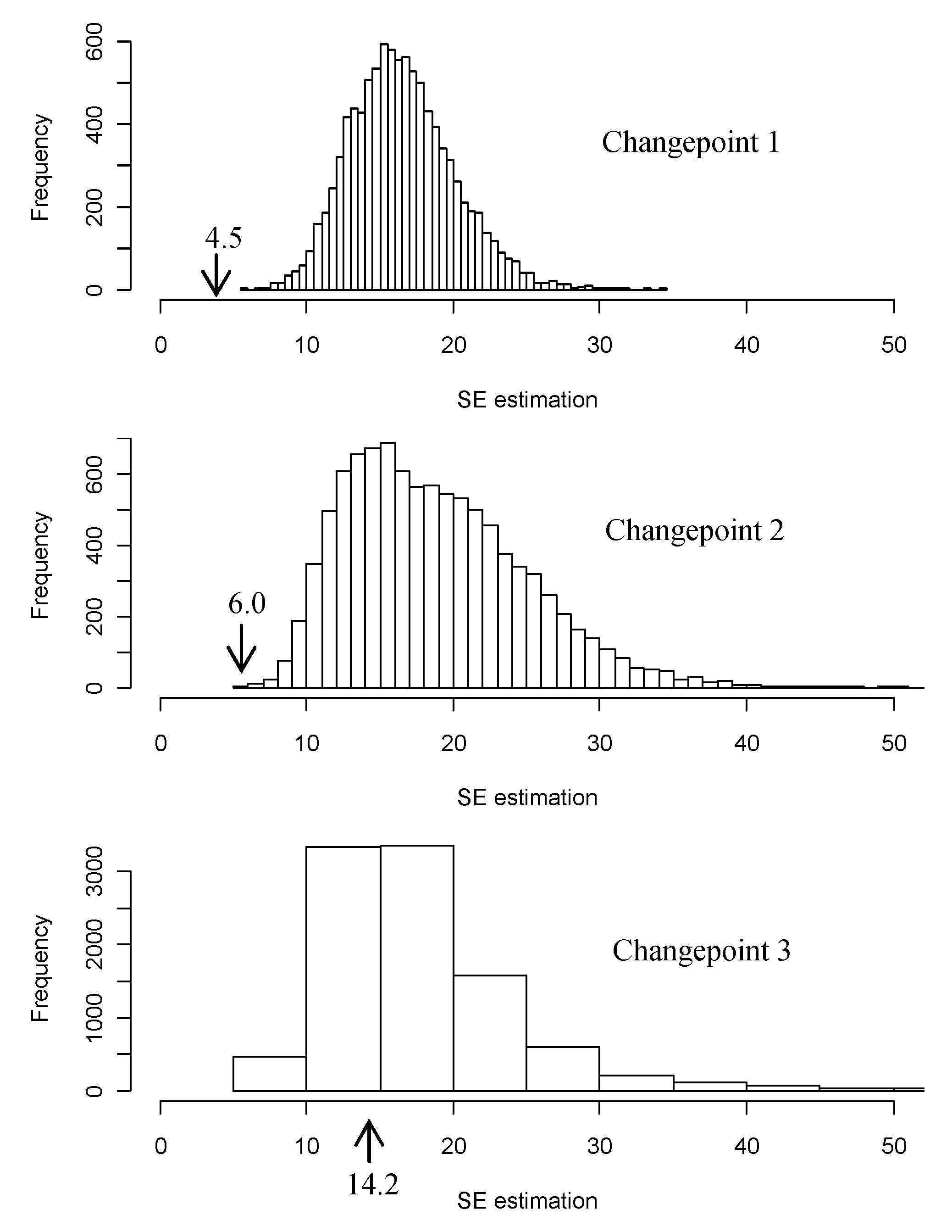
Appendix B. A Bootstrap Study of Potential Biases of the Reported SE

The Segmented algorithm (Muggeo, 2008) reports an estimated standard error (SE) of the changepoint estimation. The SE can be used to construct confidence intervals and to illustrate the stability of the changepoints. It is unclear whether the estimated SEs are reasonably close to the true SE. If large discrepancies are found, they can cast doubt on the conclusion that the changepoints are relatively stable.
In this bootstrap study, random samples of size 5,000 were repeatedly drawn (with replacement) from the dataset for Figure 7, which includes approximately 1,000,000 fixations by adult readers. Each sample then went through the analytical procedure described in the Method section, i.e., the empirical hazard function was first estimated and then modeled using the Segmented routine. The procedure was repeated 10,000 times. The study was implemented in R (v2.7), and the source code is available upon request.
Figure B. Distributions of estimated SE for the three changepoints.
Jemr 03 00008 g0a3
The bootstrap means of the changepoints were 111, 178, 240msec for change points 1, 2, and 3, respectively. Based on the 10,000 bootstrap samples, the corresponding SEs were 4.5, 6.0, and 14.2msec, respectively. Figure B shows the distributions of algorithm-estimated SEs across the 10,000 samples. The mean SEs were 16.5, 18.8, and 17.9, respectively, for the three changepoints. These figures are higher than the corresponding bootstrap estimates, marked by the arrows in the figures.
By repeatedly sampling from real data, the bootstrap study suggests that the Segmented algorithm (Muggeo, 2008) is generally conservative in estimating the standard error of a changepoint. The true confidence intervals in Figure 10 and Figure 11 may be even smaller than meet the eye.

References

  1. Aalen, O. O. 1989. A linear regression model for the analysis of life times. Statistics in Medicine 8: 907–925. [Google Scholar] [PubMed]
  2. Aalen, O. O. 1993. Further results on the non-parametric linear regression model in survival analysis. Statistics in Medicine 12: 1569–1588. [Google Scholar]
  3. Barlow, R. E., A. W. Marshall, and F. Proschan. 1963. Properties of Probability Distributions with Monotone Hazard Rate. The Annals of Mathematical Statistics 34: 375–389. [Google Scholar]
  4. Carpenter, R. H., and M. L. Williams. 1995. Neural computation of log likelihood in control of saccadic eye movements. Nature 377: 59–62. [Google Scholar] [CrossRef] [PubMed]
  5. Carpenter, R. H. S. 1988. Movements of the eyes, 2nd rev. & enlarged ed. Pion Limited. [Google Scholar]
  6. Carpenter, R. H. S. 1999. A neural mechanism that randomises behaviour. Journal of Consciousness Studies 6: 13–22. [Google Scholar]
  7. Carpenter, R. H. S. 2000. The neural control of looking. Current Biology 10: R291–R293. [Google Scholar]
  8. Carpenter, R. H. S., and S. McDonald. 2007. LATER predicts saccade latency distributions in reading. Experimental Brain Research 177: 176–183. [Google Scholar]
  9. Chechile, R. 2003. Mathematical tools for hazard function analysis. Journal of Mathematical Psychology 47: 478–494. [Google Scholar]
  10. Clifton, C., A. Staub, and K. Rayner. 2007. Eye movements in reading words and sentences. In Eye movements: A window on mind and brain. Edited by R. v. Gompel. Elsevier: pp. 341–372. [Google Scholar]
  11. Cox, D. R. 1972. Regression Models and Life Tables. Journal of the Royal Statistical Society. Series B 34: 187–220. [Google Scholar]
  12. Cutsuridis, V., N. Smyrnis, I. Evdokimidis, and S. Perantonis. 2007. A neural model of decision-making by the superior colicullus in an antisaccade task. Neural Networks 20: 690–704. [Google Scholar]
  13. Dambacher, M., and R. Kliegl. 2007. Synchronizing timelines: Relations between fixation durations and N400 amplitudes during sentence reading. Brain Research 1155: 147–162. [Google Scholar] [PubMed]
  14. Duchowski, A. T. 2003. Eye Tracking Methodology: Theory and Practice. Springer. [Google Scholar]
  15. Engbert, R., and R. Kliegl. 2001. Mathematical models of eye movements in reading: a possible role for autonomous saccades. Biological Cybernetics 85: 77–87. [Google Scholar]
  16. Engbert, R., and R. Kliegl. 2003. Microsaccades uncover the orientation of covert attention. Vision Research 43: 1035–1045. [Google Scholar]
  17. Engbert, R., A. Nuthmann, E. Richter, and R. Kliegl. 2005. SWIFT: A dynamical model of saccade generation during reading. Psychological Review 112: 777–813. [Google Scholar]
  18. Feng, G. 2003. From eye movement to cognition: Toward ageneral framework of inference. Comment on Liechty et al., 2003. Psychometrika 68: 551–556. [Google Scholar]
  19. Feng, G. 2006. Eye movements as time-series random variables: A stochastic model of eye movement control in reading. Cognitive Systems Research 7: 70–95. [Google Scholar]
  20. Feng, G. 2009. Mixed Responses: Why Readers Spend Less Time at Unfavorable Landing Positions. Journal of Eye Movement Research 3, 2: 1–26. [Google Scholar]
  21. Feng, G., K. F. Miller, H. Shu, and H. Zhang. 2009. Orthography and the Development of Reading Processes: An Eye Movement Study of Chinese and English. Child Development 80: 720–735. [Google Scholar]
  22. Findlay, J. M., and R. Walker. 1999. A model of saccade generation based on parallel processing and competitive inhibition. Behavioral & Brain Sciences 22: 661–721. [Google Scholar]
  23. Harris, C. M., L. Hainline, I. Abramov, E. Lemerise, and C. Camenzuli. 1988. The distribution of fixation durations in infants and naive adults. Vision Research 28: 419–432. [Google Scholar]
  24. Hess, K., and R. Gentleman. 2008. Muhaz: Hazard function estimation in survival analysis. Available online: http://cran.r-project.org/web/packages/muhaz/index.html.
  25. Hosmer, D. W., and S. Lemeshow. 1999. Applied survival analysis: regression modeling of time to event data. Wiley. [Google Scholar]
  26. Huey, E. B. 1908. The psychology and pedagogy of reading; with a review of the history of reading and writing and of methods, texts, and hygiene in reading. M.I.T. Press. [Google Scholar]
  27. Inhoff, A. W., and R. Radach. 1998. Definition and computation of oculomotor measures in the study of cognitive processes. In Eye guidance in reading and scene perception. Edited by G. Underwood. Anonima Romana: pp. 29–53. [Google Scholar]
  28. Johnson, N. L., S. Kotz, and N. Balakrishnan. 1994. Continuous univariate distributions, 2nd ed. Wiley & Sons. [Google Scholar]
  29. Kennedy, A., and J. Pynte. 2005. Parafoveal-on-foveal effects in normal reading. Vision Research 45: 153–168. [Google Scholar] [PubMed]
  30. Lawless, J. F. 1982. Statistical models and methods for lifetime data. Wiley. [Google Scholar]
  31. Le, C. T. 1997. Applied survival analysis. Wiley. [Google Scholar]
  32. Luce, R. D. 1986. Response times: their role in inferring elementary mental organization. Oxford University Press. [Google Scholar]
  33. Marshall, A. W., and I. Olkin. 2007. Life distributions: structure of nonparametric, semiparametric, and parametric families. Springer. [Google Scholar]
  34. Martinussen, T., and T. Scheike. 2006. Dynamic Regression Models for Survival Data (Statistics for Biology and Health). Springer. [Google Scholar]
  35. Matin, E. 1974. Saccadic suppression: a review and an analysis. Psychological bulletin 81: 899–917. [Google Scholar] [PubMed]
  36. McConkie, G. W. 1981. Evaluating and reporting data quality in eye movement research. Behavior Research Methods & Instrumentation 13: 97–106. [Google Scholar]
  37. McConkie, G. W., and B. P. Dyre. 2000. Eye fixation durations in reading: Models of frequency distributions. In Reading as a perceptual process. Edited by A. Kennedy, R. Radach, D. Heller and J. Pynte. Elsevier Science Ltd. [Google Scholar]
  38. McConkie, G. W., P. W. Kerr, and B. P. Dyre. 1994. What are "normal "eye movements during reading: Toward a mathematical description. In Eye movements in reading. Edited by J. Ygge and G. Lennerstrand. Pergamon: pp. 315–327. [Google Scholar]
  39. McConkie, G. W., D. Zola, J. Grimes, P. W. Kerr, N. R. Bryant, and P. M. Wolff. 1991. Children’s eye movements during reading. In Vision and visual dyslexia. Edited by J. F. Stein. Macmillan Press: pp. 251–262. [Google Scholar]
  40. McDonald, S. A., R. H. S. Carpenter, and R. C. Shillcock. 2005. An anatomically constrained, stochastic model of eye movement control in reading. Psychological review 112: 814–840. [Google Scholar]
  41. Morrison, R. E. 1984. Manipulation of stimulus onset delay in reading: Evidence for parallel programming of saccades. Journal of Experimental Psychology: Human Perception & Performance 10: 667–682. [Google Scholar]
  42. Moscoso Del Prado Martin, F. submitted. A Theory of Reaction Time Distributions. Behavior and Brain Sciences.
  43. Muggeo, V. M. R. 2008. segmented: An R package to fit regression models with broken-line relationships. R News 8: 20–25. [Google Scholar]
  44. Munoz, D. 2002. Saccadic eye movements: overview of neural circuitry. In The Brain’s eye: Neurobiological and clinical aspects of oculomotor research. Edited by J. Hyona, D. P. Munoz, W. Heide and R. Radach. Elsevier: pp. 89–96. [Google Scholar]
  45. Nakahara, H., K. Nakamura, and O. Hikosaka. 2006. Extended LATER model can account for trial-by-trial variability of both pre-and post-processes. Neural Networks 19: 1027–1046. [Google Scholar]
  46. Pynte, J., and A. Kennedy. 2006. An influence over eye movements in reading exerted from beyond the level of the word: Evidence from reading English and French. Vision Research 46: 3786–3801. [Google Scholar]
  47. R Development Core Team. 2008. R: A language and environment for statistical computing. R Foundation. [Google Scholar]
  48. Ratcliff, R. 1979. Group reaction time distributions and an analysis of distribution statistics. Psychological Bulletin 86: 446–461. [Google Scholar]
  49. Rayner, K. 1986. Eye movements and the perceptual span in beginning and skilled readers. Journal of Experimental Child Psychology 41: 211–236. [Google Scholar]
  50. Rayner, K. 1998. Eye movements in reading and information processing: 20 years of research. Psychological Bulletin 124: 372–422. [Google Scholar] [CrossRef] [PubMed]
  51. Rayner, K. 2009. Eye movements and attention in reading, scene perception, and visual search. The Quarterly Journal of Experimental Psychology. [Google Scholar] [CrossRef] [PubMed]
  52. Reddi, B. A., K. N. Asrress, and R. H. Carpenter. 2003. Accuracy, information, and response time in a saccadic decision task. J Neurophysiol 90: 3538–3546. [Google Scholar] [CrossRef] [PubMed]
  53. Reichle, E. D., A. Pollatsek, D. L. Fisher, and K. Rayner. 1998. Toward a model of eye movement control in reading. Psychological Review 105: 125–157. [Google Scholar] [CrossRef]
  54. Reichle, E. D., A. Pollatsek, and K. Rayner. 2006. E-Z reader: A cognitive-control, serial-attention model of eye-movement behavior during reading. Cognitive Systems Research 7: 4–22. [Google Scholar] [CrossRef]
  55. Reichle, E. D., K. Rayner, and A. Pollatsek. 1999. Eye movement control in reading: accounting for initial fixation locations and refixations within the E-Z Reader model. Vision Research 39: 4403–4411. [Google Scholar] [CrossRef]
  56. Reichle, E. D., K. Rayner, and A. Pollatsek. 2003. The E-Z Reader model of eye-movement control in reading: Comparisons to other models. [Google Scholar]
  57. Reichle, E. D., T. Warren, and K. McConnell. 2009. Using E-Z Reader to model the effects of higer-level language processing on eye movements during reading. Behavioral and Brain Sciences Psychonomic Bulletin & Review 16: 1–21. [Google Scholar]
  58. Reilly, R. G., and J. K. O’Regan. 1998. Eye movement control during reading: A simulation of some word-targeting strategies. Vision Research 38: 303–317. [Google Scholar]
  59. Richter, E. M., R. Engbert, and R. Kliegl. 2006. Current advances in SWIFT. Cognitive Systems Research 7: 23–33. [Google Scholar]
  60. Robert, C. 1991. Generalized inverse normal distributions. Statistics & Probability Letters 11: 37–41. [Google Scholar]
  61. Sereno, S. C., and K. Rayner. 2003. Measuring word recognition in reading: eye movements and event-related potentials. Trends in Cognitive Sciences 7: 489–493. [Google Scholar] [PubMed]
  62. Suppes, P. 1990. Eye-movement models for arithmetic and reading performance. In Eye movements and their role in visual and cognitive processes. Edited by E. Kowler. Elsevier: Vol. 4, pp. 455–477. [Google Scholar]
  63. Suppes, P. 1994. Stochastic models of reading. In Eye movements in reading. Edited by J. Ygge and G. Lennerstrand. Pergamon Press: pp. 349–4364. [Google Scholar]
  64. Suppes, P. M., Laddaga Cohen R., J. Anliker, and R. Floyd. 1983. A procedural theory of eye movements in doing arithmetic. Journal of Mathematical Psychology 27: 341–369. [Google Scholar]
  65. Tukey, J. W. 1977. Exploratory Data Analysis. Addison-Wesley. [Google Scholar]
  66. Van Zandt, T. 2000. How to fit a response time distribution. Psychonomic bulletin & review 7: 424–465. [Google Scholar]
  67. Van Zandt, T., and R. Ratcliff. 1995. Statistical mimicking of reaction time data: Single-process models, parameter variability, and mixtures. Psychonomic Bulletin & Review 2: 20–54. [Google Scholar]
  68. Wolverton, G. S., and D. Zola. 1983. The temporal characteristics of visual information extraction during reading. In Eye movements in reading: Perceptual and language processes. Edited by K. Rayner. Academic Press: pp. 41–52. [Google Scholar]
  69. Yang, S.-n. 2006. An oculomotor-based model of eye movements in reading: The competition/Interaction model. Cognitive Systems Research 7: 56–69. [Google Scholar]
  70. Yang, S.-N., and G. W. McConkie. 2001. Eye movements during reading: a theory of saccade initiation times. Vision Research 41: 3567–3585. [Google Scholar]
Figure 1. Hazard Functions of Normal, Lognormal, and Gamma Distributions with the Same Means and Standard Deviations.
Jemr 03 00008 g001
Figure 2. Hazard Function and the Probability Density. Function: The Dundee Corpus.
Jemr 03 00008 g002
Figure 3. Hazard Functions by Language.
Jemr 03 00008 g003
Figure 4. Developmental Comparison of Hazard Functions.
Jemr 03 00008 g004
Figure 5. Individual Differences in Hazard Function: 10 Adult Readers from the Dundee Corpus.
Jemr 03 00008 g005
Figure 6. Effects of Word Frequency on Hazard Function of Fixation Duration (Dundee corpus).
Jemr 03 00008 g006
Figure 7. Effect of Word Length (Dundee corpus).
Jemr 03 00008 g007
Figure 8. Hazard Functions for Fixations to be Followed by a Forward, Refixation, and Regressive Saccade.
Jemr 03 00008 g008
Figure 9. Hazard functions and pdf’s of reading fixation duration based on pooled reading data for 3rd- and 5th-grade children and adults. Moving averaging is used to smooth the hazard function after 400msec.
Jemr 03 00008 g009
Figure 10. A-B. Summary of Estimated Changepoint Locations. Panel A includes estimates based on different datasets. All estimates in Panel B are based on the Dundee corpus.
Jemr 03 00008 g010
Figure 11. A-B. Summary of Estimated Slopes of Segmented Linear Regression. Data in Panel A are from independent corpora. Data in Panel B are from the Dundee corpus.
Jemr 03 00008 g011
Table 1. Summary of characteristics of the datasets used in the study.
Jemr 03 00008 i001

