Abstract
This paper aims at analyzing nonlinear dependence between fractionally integrated, chaotic precious metal and oil prices and volatilities. With this respect, the Markov regime-switching fractionally integrated asymmetric power versions of generalized autoregressive conditional volatility copula (MS-FIAPGARCH-copula) method are further extended to multi-layer perceptron (MLP)-based neural networks copula (MS-FIAPGARCH-MLP-copula). The models are utilized for modeling dependence between daily oil, copper, gold, platinum and silver prices, covering a period from 1 January 1990–25 March 2022. Kolmogorov and Shannon entropy and the largest Lyapunov exponents reveal uncertainty and chaos. Empirical findings show that: i. neural network-augmented nonlinear MS-FIAPGARCH-MLP-copula displayed significant gains in terms of forecasts; ii. asymmetric and nonlinear processes are modeled effectively with the proposed model, iii. important insights are derived with the proposed method, which highlight nonlinear tail dependence. Results suggest, given long memory and chaotic structures, that policy interventions must be kept at lowest levels.
1. Introduction
Precious metal (PM) and oil prices have significant roles in the real sector in addition to the financial markets. Further, forecasting and foreseeing the oscillations in oil and PM prices, in addition to investigating their interrelations, is of critical importance for various participants in economies. This includes administrators in the real sector, investors in the financial sector, and policymakers in the public sector. Even if gold and silver were popular options among PMs until recent years, nowadays platinum has gained importance for financial investment portfolios. Precious metals are also utilized effectively and commonly in a wide set of industries, ranging from semiconductor/chip production/electronics to construction.
Precious metals face noteworthy demand from manufacturing and the ornaments industries, in addition to being considered as a measure of wealth stock. In addition to such industries, precious metals (hereafter PM) are included in the portfolios of institutional and individual investors in the finance sector because they are viewed as a safe investment during periods of recessions, stagnations, and crises. Further, the selected metals in the study—gold, silver, platinum, and copper—especially face significant demand from the production side through industrial demand. It is noted that, especially during the COVID-19 period, these four metals showed significant fluctuations compared to other various metals. When evaluated together with oil price fluctuations, while a rise in oil prices causes supply-side inflation, the platinum, copper, silver and gold prices fluctuate with inflation due to two main factors. First, during sharp periods of recessions and crises, to balance their portfolio, investors include such assets with safe-haven expectations. Second, as economies start to open, precious metals are demanded even more in many industries. Nevertheless, the inclines in shipment costs, in addition to chip shortages, still lead to drastic supply shortages today. These are also coupled with inclines in PM prices. Recent evidence shows that periods of inflation and stagflation drive their prices, especially during economic crisis periods. Given the fact that PMs have different uses in different sectors including electronics, automobiles, and even dentistry components, they are subject to increased demand. This drives their prices and fluctuations due to economic conditions that affect the manufacturing industries. Due to the electrical conductivity, ductility, and malleability of PM, they are used in many applications, including radar equipment, satellites, and electronics in addition to semiconductors and electronic circuits. As an example of a typical year-period, platinum demand, when divided by use, saw 38% for auto-catalysts, 31% for jewelry, and 6% for exchange-traded fund (ETF) investments in 2011 [1]. Moreover, among the four PM’s analyzed in the study, gold, silver, and platinum attract additional attention from the jewelry and ornament industries.
The construction, electrical, automotive, and manufacturing industries are known for being sensitive to the volatility in prices of oil and precious metals. Among the four PMs used in the study, copper is largely demanded by the construction industry and industrial machinery production industries, in addition to its use in transportation and vehicles, not to mention energy generation facilities and the transportation of electricity. If an overall evaluation is provided, the four PMs are subject to strong price oscillations. This is due to economic business cycles that characterize investment behavior towards portfolio diversification, inflationary periods in the economy, and also due to economic crises periods coupled with strong oil price fluctuations. These factors make the investigation of the oil price and volatility interrelations with selected PMs especially important.
In addition to demand conditions, there are some other factors affecting the PM and oil prices. Hence, PM and oil prices are economic [2], speculative [3], non-economic factors. Examples include the Gulf war, and geopolitical tensions [4]. In recent years, the upsurge of speculative activities is also observed to lead to inclines in volatility and uncertainty in the gold, platinum, copper, and silver prices, in addition to oil prices [5]. Nevertheless, uncertainty and volatility in the prices of the selected PM set in the study could have strong implications on the investment decisions, in addition to the decisions and costs of manufacturers in industrial production. Furthermore, during the COVID-19 lockdown period, the uncertainty of PM prices became more evident in addition to sudden fluctuations in their prices. As will be discussed in the literature section, the recent literature provides evidence of relations between PMs and oil prices including common tail risk in addition to spillover effects from oil to PMs, especially during COVID-19. Additionally, PMs are shown to provide hedge potential for oil price jumps during crises and deep recession periods.
The PM and oil returns and volatilities can exhibit persistence and nonlinear behavior [6,7,8] during business cycles with expansionary and recessionary stages, the furthest extent of which are the boom and crisis periods. Each stage could have a uniqueness in terms of duration in addition to its distinct distributional characteristics; these are subject to being governed by regime switches [9,10], a phenomenon which leads to nonlinear and asymmetric behavior. For instance, during crises and/or during high-volatility regimes, the financial return series can become less persistent compared to the boom stage and/or low volatility regime [11], or when the duration of phases of economic expansion is longer than that of periods of crisis. The asymmetry between the periods of high–volatility and low–volatility regimes can be explained as also being dependent on the length of time. According to Cuddington and Jerrett [12], if the volatility in metal prices over the last 200 years were to be categorized by four main cycles that exhibited persistence between 20 and 70 years, the fourth super-cycle would be stated to be started in 1999 which continues today [13,14].
In this paper, two different regimes, low and high volatility, will be investigated to determine whether there is evidence of variation in the dependence and persistence structure between oil and PM returns, whether there is tail dependence, whether copula parameters are greater than previous ones after the change point, and whether a contagion impact occurs. Firstly, the evidence of chaotic behavior and uncertainty for the changes in oil price and the return of precious metals will be explored by Kolmogorov and Shannon entropy tests, and the Lyapunov exponent test. For the Kolmogorov and the Shannon entropy tests, it will be explored whether the Eckmann–Ruelle condition is satisfied. Moreover, the Markov-switching fractionally integrated asymmetric power GARCH (MS–FIAPGARCH), and its multi–layer perceptron (MLP)—augmented version, the MS–FIAPGARCH–MLP model will be integrated into copulae to obtain the MS–FIAPGARCH–MLP–copula method. If the volatilities of PMs and oil prices are interdependent, the MS–FIAPGARCH–MLP models will determine the contagion, persistence, nonlinear, and/or asymmetric behavior in PM and oil price. For comparative purposes and to evaluate the results, the MS–FIAPGARCH–copula method is applied. These methods will reveal the contagion impact, asymmetric behavior, and persistence of PM and oil price volatility in distinct regimes characterized by high or low volatility.
Asymmetric behavior, persistence, and contagion impacts were analyzed separately via various methods in many papers. Nonetheless, these methods did not provide an overview of all impacts simultaneously. The MS–FIAPGARCH–copula and the MS–FIAPGARCH–MLP–copula methods are capable of providing and evaluating such impacts simultaneously. Some papers used unit root tests to determine the PM volatility persistence. However, the unit root testing methods are known for having insufficiencies under certain states. First, these tests exhibit lower power in the state of high persistence which causes an over–acceptance of the unit root behavior [15,16,17]. Second, omittance of structural breaks leads to inflated parameter estimates which measure persistence [18].
To test the volatility and non–linear behavior in PM and oil prices, some papers used various GARCH methods. There are some insufficiencies in this methodology. Firstly, the outliers can be seen in both in oil and PM price series. If the phases of the cycle and outliers are not explored, the estimated parameters can become misleading and incorrect. The outliers also influence the estimation of and the model selection of GARCH family methods [19,20] and could mistakenly result in hiding heteroscedasticity or the suggestion of conditional heteroscedasticity [21]. Moreover, the performance of out–of–sample forecasts obtained from GARCH models is affected if nonlinearities and regime dependencies are not taken into account [22]. To control the problem caused by outliers various methods have been proposed. Ané et al. [23] proposed an outlier–augmented–GARCH and estimation procedure for such methods are discussed. For the detection of outliers, Charles and Darné [24,25] suggested employing the Laurent et al. [26]’s outlier detection method. In the condition of outliers, Bildirici and Ersin [6,7,8] suggested estimating the volatility in oil prices with the LSTAR–LST–GARCH–RBF and LSTAR–LST–GARCH–MLP methods. Additionally, Bildirici and Ersin [7,8,9] showed that, in the case of the business cycle and outliers, the MS–FIAPGARCH and MS–FIAPGARCH–MLP methods are more efficient than the other GARCH methods.
This paper has important contributions. For econometric modeling, the paper distinguishes different regimes and their effects on analyzing the oil prices and precious metals (PM) which are shown to be fractionally integrated. Further, the paper determines the regime-dependent fractional integration, copulae-based contagion and tail-dependence among PM’s and oil prices with MS–FIAPGARCH–copula and MS–FIAPGARCH–MLP–copula methods. The methods also allow for investigation of persistence and spillover effects between PM’s and oil prices. Methodologically, the MS–FIAPGARH method is generalized to MS–FIAPGARH–copula and MS–FIAPGARH–MLP–copula methods, where the latter is a regime–dependent neural network–augmented model. The recent literature following the copulae approaches to contagion is extended to regime dependency in the coefficients of tail dependence and copula. Examples include the studies of Chan-Lau et al. [27], Forbes and Rigobon [28], Boubaker and Sghaier [29], and Bildirici [30]. As for the application aspect, the proposed method has significant gains by augmenting the forecasting capabilities with neural networks. This paper is among the first papers employing the MS–FIAPGARH–MLP–copula method to evaluate the contagion and its impacts on PM and oil price volatility.
2. Literature Review
The works of Mckenzie et al. [31], Liao and Chen [32], Tully and Lucey [33], Kang et al. [34], Morales and O’Callaghan [35], Cochran et al. [36,37], Ewing and Malik [38], Arouri et al. [3], Bildirici and Ersin [6,8,9], Chkili et al. [39], Gil-Alana and Tripathy [5], Tiwari and Sahadudheen [40], and Behmiri and Manera [41] examined the volatilities of oil and precious metal using the GARCH methods. The overview of the studies above provides insights as a basis for investigating fractional integration and asymmetric nonlinear behavior in the volatility processes of PMs and oil prices. Gil-Alana and Tripathy [5], for metal markets, tested the leverage effect and persistence by employing the GARCH family methods and determined an important level in the persistence of volatility. They explained the nonlinearity using the TGARCH model for 7 PMs and with EGARCH model for 10 PMs. Mckenzie et al. [31] explored the volatility of PMs by employing the PARCH model, but they did not determine asymmetric effects in metal markets. Arouri [3] showed the impact of structural breaks, whereas Liao and Chen [32] analyzed the relationship amid gold and oil prices in Taiwan by using the TGARCH model. Tully and Lucey [33] showed the leverage effects with the APGARCH models. Kang et al. [34] explored the persistence in the oil prices by employing GARCH models. Morales and Andreosso-O’Callaghan [35] tested the PM volatility dynamics with GARCH and EGARCH models, and pointed out the persistency in the relation between returns of PMs during the 2008 crisis in contrast to their weak persistence during the Asian crisis.
Fractional integration has a central role in the determination of long memory in PM and oil prices. As a basis, Arouri et al. [3] investigated the fractional integration and long memory characteristics for platinum, silver and gold with the FIGARCH model and showed the existence of dependence amid investigated PMs. Cochran et al. [36] tested the threshold effects for some metals. According to their results, the DT-FIGARCH model determined the nonlinearity of metal returns and volatilities. Moreover, they found that long memory returns depend on the regime. Conversely, in the short memory, parameter returns of platinum copper, and silver are unaffected by shifts in the regime. Cochran et al. [37] examined the volatilities of some metals using the FIGARCH model and their findings revealed the importance of modeling fractional integration in the metal markets.
A certain set of papers provided evidence in favor of nonlinearity. Ewing and Malik [38] used bivariate and univariate GARCH models and they examined the gold and oil price volatility by combining structural breaks, finding strong evidence of volatility transmission amid returns of oil and gold by incorporating structural breaks to the conditional variance processes. Chkili et al. [39] examined the volatilities of oil, gold, gas, and silver with various GARCH methods and determined an inverse leverage effect in silver and gold prices. Tiwari and Sahadudheen [40] explored the association amid gold and oil prices by using GARCH methods. The results confirmed positive impact of rises in oil prices on gold price. [40] also showed that EGARCH model underlined the importance of asymmetric effects and helped on the determination that shocks with different signs led to dissimilar impacts on gold prices. Behrimi and Manera [41] showed the roles of oil shocks and outliers on volatility transmission mechanisms between various PM’s. Mensi et al. [42] showed volatility transmission amid oil and previous metals and obtained safe–haven characteristics in the Asian crisis and during COVID-19. Hammoudeh and Yuan [43] tested the volatility in prices of silver, copper, and gold by employing GARCH type–models and the presence of the shocks by including oil prices. Diaz [44] used four combinations of fractional integration (FI) models to estimate the dependence in the returns of platinum and palladium.
Das et al. [45] explored the impacts of oil price jumps on PMs and showed that the inclines in oil volatility led to volatility in PM prices in addition to putting forth the potential of PMs as hedging tools. Ahmed et al. [46] investigated tail risk and spillover effects between crude oil and PMs using GARCH models and their findings showed time–varying effects in addition to the acceleration of spillover risk, especially during periods of crisis. Bentes [47] explored the volatility persistence of PM prices before and throughout COVID-19 in the direction of evaluating hedge and safe–haven characteristics. Dinh et al. [48] demonstrate the negative and positive effects of economic factors on PM prices. Mensi et al. [49] investigate currency market and PM market links and show that PMs have strong hedge potential along with spillover effects from oil to PMs, which alter depending on the magnitude and the direction of the change. In a recent study, Septhon [50] showed the hedge effectiveness of PMs against inflation. Kaczmarek et al. [51] explore a large set of safe–haven asset candidates including various PMs; in contrast to the literature, they concluded that no safe–haven property exists for the evaluated PMs. If the above–mentioned literature is overviewed, the characteristics of the PM and oil relation necessitate the investigation of interrelations and contagion effects between PM and oil in combination with fractional integration and nonlinearity with more recent techniques that capture not only fractional integration and nonlinearity, but also tail dependence and contagion relations.
A selected set of papers analyzed the volatility in oil or gold price by combining MSGARCH or LSTARGARCH and neural network methods. One study conducted by Bildirici and Ersin [6] used the LSTARLSTGARCH family of models and their neural networks variants to examine oil price volatility. According to their findings, nonlinearity, volatility, and asymmetry in oil is effectively modeled with MLP based versions. Bildirici and Ersin [8] suggested MLP and RBF based neural network–augmentation of nonlinear LSTARLSTGARCH models to achieve gains in forecasting capabilities if daily oil prices are to be modeled. Their results confirmed that the RBF and MLP extensions of the LSTARLSTGARCH models provided a significant improvement in volatility modeling and forecasting. Bildirici and Ersin [7] evaluated the Markov–switching GARCH–MLP methods and their results exhibited enhanced performance in forecasting the volatility in daily returns for the international gold market. Jahanshahi et al. [52] explore the financial hyperchaotic structures with coexisting attractors. Bildirici and Sonüstün [53] determine the chaotic structure in bitcoin and three different PMs’ prices. Bildirici [54] inspects the chaotic dependence between PMs, oil and COVID-19 MS–GARCH–MLP–copula models.
From the standpoint of the contagion effects, the stock markets have been tested in many papers by employing various econometric approaches. A set of papers utilize dynamic conditional correlation DCC) method to cover the time-varying structure in the correlations [55,56,57,58,59], while a certain set of other papers uses the switching models [60]. These methods are insufficient since they do not allow asymmetry in the dependence parameters [61]. To this extent, some papers used copula methods to analyze contagion with tail dependence. Among these, a large set of papers in this respect used the Archimedean copula [62]. The study by Rodriguez [63] was among the first studies to suggest time–varying copula. Boubaker and Sghaier [64,65] investigated the existence of a change–point in the dependence based on copula. Refs. [64,65] found the signal of instability in both tail dependence and copula parameters. By applying TAR–TR–TGARCH–copula, Bildirici [30] studied co–movement among the expectations of the investors, oil price and stock return volatility and determined presence of nonlinear tail dependence among the selected variables. By MSGARCH–MLP methods, Bildirici [54] tested the co–movement and contagion behavior among returns of precious metals, oil price and COVID-19–infected persons for the 30 December 2019, 26 October 2020 period with MS–GARCH–MLP–copula model and determined co–movement and contagion structure among the selected variables. Bildirici’s findings support the nonlinear contagion and causality between the gold and oil prices, the VIX, currency exchange rates, and stock market returns.
3. Methodology
The fractionally integrated asymmetric power generalized autoregressive conditional heteroskedasticity (FIAPGARCH) model is a conditional model that allows integrating fractional integration, in addition to asymmetric power terms, into GARCH–type conditional heteroskedasticity models. The Markov regime–switching (MS) concept of Hamilton [11] is introduced to FIAPGARCH processes to let them have regime–dependent dynamics in two or more distinct regimes to achieve the MS–FIAPGARCH model. The model is used for modeling marginal distributions of time series which are further utilized in copula modeling. In this paper, a novel model which is based on the augmentation of MS–FIAPGARCH–copula model with multi–layer perceptron (MLP) neural networks. The MS–FIAPGARCH–MLP–copula aims at capturing long memory and persistence characteristics that possess different characteristics in two distinct regimes. The model also allows the modeling of tail dependence with copulae functions within each regime. The inclusion of MLP’s to each regime aim at augmenting the forecasting and generalization capacity. Therefore, two models will be utilized in this study. The first benefits from MS, FIAPGARCH and copula, while the second further augments the first with MLPs to improve the generalization, forecasting and modeling of tail dependence.
3.1. MS–FIAPGARCH Model
Following [7,9,11,54], a regime–switching GARCH model with Markov-switching is,
where xt is a daily return series, Equations (1 defines conditional mean, Equations (2) and (3) define conditional variance for time series xt. The model assumes a Markov regime–switching MS–ARMA(r,m) process with AR and MA orders of r and m in Equation (1) and a regime–switching GARCH(p,q) process where p and q define orders of ARCH and GARCH terms in Equation (2) which are assumed as p = 1, q = 1. The non–negativity constraints for the > 0 are assumed and obtained through the following,
and is attained through iteration, where,
Two approaches, Francq and Zakoian [66] and Henneke et al. [67] are separated in terms of the descriptions of and , and the study assumes the Francq and Zakoian model [66]. The MS–FIAPGARCH model is achieved by further extending the MS–GARCH model to asymmetric power and fractional integration. Therefore, the MS–FIAPGARCH extends conditional variance function in Equation (5) with regime–dependent power terms and long–memory characteristics. Following the method of [9,11], the MS–FIAPGARCH is presented as,
with , , , and non–negativity restrictions. The is the power term and is regime–specific and is bounded fractional differentiation parameter. Regime changes are governed by st = 1, 2,…, m; for m number of regimes, as a function of the unobservable Markov process. The asymmetry is captured with in each st regime, so that the negative and positive innovations with similar magnitudes lead to asymmetric responses in the regime–specific conditional variance processes. The regimes of the conditional variance process—st—are achieved by maximizing the log–likelihood (LL) function,
for a return series and is the conditional probability that is to be achieved through iteration,
3.2. MS–ARMA–GARCH–MLP and MS–ARMA–FIAPGARCH–MLP Models
The multi–layer perceptron (MLP) method consists of the input layer, one or more hidden layers and an output layer [7]. In the MS–ARMA–GARCH–MLP model of Bildirici and Ersin [7], the conditional mean is modeled as Equation (1), while the conditional variance is modeled as Equation (9) below which augments the MS–GARCH model with MLP–type neural networks,
for st with i = 1,…, m regimes which are directed by an unobservable Markov process,
so that the variances are a function of probability of being at regime state i which is conditional on the normalized residuals. The model assumes h number of neurons of the form of sigmoid activation functions,
with ~ uniform . is the filtered probability constructed as,
in which, zt−d is the normalized residuals,
The is recursive which is gathered via initiating , and the assumption of logistic function 1/(1 + exp(−x)) leads to favorable characteristics for optimization, given that the logistic function is twice–differentiable, continuous and [0, 1] bounded. Based on [7], in case of , the transition probability was taken as,
hence, the recursive process is obtained by building as given by Bildirici and Ersin [7].
3.3. MS–ARMA–FIAPGARCH–MLP
Bildirici and Ersin [7] obtain the MS-ARMA-GARCH-Neural Network model by introducing MLP type neural networks in MS-GARCH model given in Equations (1)–(3). To further capture fractional integration and asymmetric power properties, the model is generalized to MS–ARMA–FIAPGARCH–MLP by augmenting Equations (1)–(6) with MLP neural networks given in Equation (9). The model is achieved as,
where,
is the logistic activation function [7]. Further, ~ uniform and is the filtered probability,
with zt−d being normalized . The dynamics of transition is determined through the conditional probability which is given as,
3.4. MS–ARMA–FIAPGARCH–Copula and MS–ARMA–FIAPGARCH–MLP–Copula
Both MS–ARMA–FIAPGARCH–MLP–copula and MS–ARMA–FIAPGARCH–copula methods provide the exploration of contagion structure through various forms of tail dependence functions among analyzed variables. Among these, one of the most common ones is the symmetrized Joe Clayton (SJC) [54,68],
where is the lower, is the upper tail copula parameters [29,69]. Another common copula is the Joe Clayton (CJC) which also has interesting properties,
where and and . Similar to the SJC copula [68], the upper and lower tail dependences are gathered by JC copula [68]; the dependence is asymmetric if symmetric and, in the case of , the dependence becomes symmetric [29,30,54,63].
4. Empirical Results
4.1. Data
The sample covers daily observations for the 1 January 1990–25 March 2022 period and the dataset consists of daily prices of oil, copper, silver, gold and platinum and is obtained from the Bloomberg database. For all commodities evaluated in the analysis, their generally accepted units are utilized, and all are reported in USA dollars (USD). Oilt is the per barrel USD Brent oil price, Coppert is the USD price per 1 lbs. of of copper. Goldt, Platinumt and Silvert are quoted per 1 ounce USD price, and they represent gold, platinum and silver price per 1 ounce. In the analysis, all variables are in daily percentage returns. Further, the dataset is divided into training, test, forecast sub–samples with 80–10–10 percentages. The total sample size is n = 8411.
The justification of daily data use is based on the work of Reboredo and Rivera–Castro [70], who accepted that daily data is more appropriate in exploring contagion due to the fact that shocks are transmitted immediately and this also leads high speeds in contagion after a shock. However, the transmission and contagion could also expire very rapidly in couple of days. Further, the study assumes working days, i.e., five days per week.
The analysis comprises the following five stages,
- i.
- Exploring data with descriptive statistics. Employing Hsieh and Tsay tests to determine nonlinearity [71,72].
- ii.
- Examining presence of chaotic behavior through Lyapunov exponents, Kolmogorov–Shannon entropy tests. Exploring whether the Eckmann–Ruelle [73] condition holds.
- iii.
- Determination of the number of regimes, calculating regime durations and regime transition probabilities [11].
- iv.
- Estimation of MS–FIAPGARCH–copula and MS–FIAPGARCH–MLP–copula models which integrate fractional integration into the MS–GARCH–MLP model of [54].
- v.
- Determination of contagion effects, as well as the persistence and dependency behavior.
- vi.
- Obtaining the forecast results and evaluating forecast performances.
Forecasting evaluation is crucial to assessing the effectiveness of the models and to evaluating whether differentiated (or improved) results exist.
4.2. Results
4.2.1. Descriptive Unit Root, ARCH Effects and Nonlinearity Tests
The descriptive statistics for oil, gold, copper, silver and platinum % returns are reported Table 1. Among the analyzed variables, platinum has the lowest (0.173) and oil has the highest standard deviation (0.687). The low value of platinum may be an effect of its lower rate of industrial usage, and the high returns of gold could be originated from the usage of gold as a long–run hedge counter to inflation or economic crises which is thought to have reflections on its monetary value.

Table 1.
Descriptive statistics.
Table 1 also exhibits that the % returns of copper, platinum and oil are negatively skewed. For all % return series, the JB, Q(5), R/S, Runs and Lo’s R/S test results determined non–normality, persistence and non–linearity at a 1% statistical significance level. In Table 2, the results of ADF and ARCH–LM tests are shown. For all series, the H0 hypothesis of a unit root is rejected at conventional significance levels and ADF tests confirmed that the variables are I(0) stationary. The ARCH–LM test reveals ARCH–type heteroskedasticity in data, which confirms the necessity of integration of ARCH–type processes in addition to nonlinearity to analyze the series investigated.
Table 2.
Unit root and ARCH–type heteroskedasticity test results.
The ARCH effects determined the necessity of the utilization of models aiming at modeling the conditional heteroskedasticity under consideration. In the next step, the Hsieh and Tsay tests [71,72] were applied to testing the nonlinearity reported in Table 3. Two different tests were applied to obtain robust results for different forms of nonlinearity.
Table 3.
(a) Tsay Nonlinearity Test. (b) Hsieh Test Results.
The Tsay test results favor nonlinearity in the investigated series. The test is known to capture cases of additive nonlinearity, but also known to have relatively less power against multiplicative nonlinearity [71,72]. Hsieh test is applied to test if the third–order moments parameters are different from zero. The Hsieh [72] test confirms the nonlinearity in the five series investigated.
4.2.2. Chaotic Behavior Tests
In the next step, the Lyapunov exponent (LE), Kolmogorov entropy (KE) and Shannon entropy (SE) tests were employed. The results are presented in Table 4.
Table 4.
The results of Lyapunov exponent, and Kolmogorov and Shannon entropy testing.
The positive LE values showed a chaotic structure but not deterministic chaotic structure due to exponents being measured as LE < 1. Under these conditions, the predictability of the analyzed series is expected to be very low. The results show that the variables follow chaotic structures in addition to being nonlinear stochastic processes. The results for % oil returns are in accordance with the results of Adrangi and Chatrath [74], and Bildirici and Sonüstün [75] who confirmed the existence of chaotic structure for % oil price returns. In addition, the results also confirm those from Bildirici and Sonüstün [75] in terms of gold, silver and copper % returns.
SE and KE tests reveal important characteristics of data in terms of uncertainty and in terms of following random processes in addition to complexity. The variable is accepted as following a random or uncertain process as the value of the entropy statistic becomes 1 and, if the calculated entropy statistic is 0, the results favor perfect certainty. Regarding the analyzed variables, the results do not favor certainty and they confirm the series analyzed as random and uncertain processes. Similar to these results, for oil price during COVID-19, Bildirici [54] found the results of the Shannon and Kolmogorov entropies as 0.932 and 0.882, respectively, approaching unity during that period. The difference between the coefficients of uncertainty was due to the period analyzed, and the uncertainty coefficients decreased due to their covering a relatively very large period in the sample of this study.
4.2.3. Model Selection for MS–GARCH–Copula
The test results suggest the rejection of the single–regime GARCH(1,1), APGARCH(1,1) and FIAPGARCH(1,1) models, and the two–regime MS–FIAPGARCH and MS–FIAPGARCH–MLP models were accepted as candidate models. To model tail dependency and contagion, four different copulae are utilized: i. Clayton, ii. Gumble, iii. symmetrized Joe Clayton and, iv. Student’s t. Following the recommendations of [54,76], the selection of the copula in models is conducted by employing i. deviance information criterion (DIC) and, ii. the acceptance statistic of [76]. The results are reported in Table 5. Symmetrized Joe Clayton produced the highest DIC (least negative) than any other copulae applied. Gumble produced the lowest DIC (i.e., the most negative) in addition to providing the highest acceptance statistic, that is, 52%. Zhu et al. [76] and Bildirici [54] found Student’s t functions providing high acceptance values. In contrast to these findings, Student’s t and symmetrized Joe Clayton copulae led to relatively lower acceptance rates for our sample and for the analyzed commodity prices.
Table 5.
Copula Selection Tests.
4.2.4. MS–FIAPGARCH–Copula Estimation Results
In Table 6, the transition probabilities of the estimated models are reported. Given the fractional integration parameter estimates, the second regime (R2) is characterized with higher persistence, except for gold % returns, for the majority of commodities relative to the first regime (R1). The overall investigation favors R1 as the high–variance regime with lower returns and R2 as the low–variance regime with higher returns. Hence, the R2 represents the low variance regimes with higher returns compared to the high–variance R1 with lower returns. Further, given the regime switching probabilities, persistence in R2 is relatively higher compared to R1 for all commodities. Similar results for precious metals can be seen in the works of Cashin [77] and Rossen [78], which determine the asymmetry of commodity price cycles. Another point is that the MS–FIAPGARCH model is capable of providing regime–dependent characteristics given above which are among the major advantages over its single–regime variant.
Table 6.
MS–FIAPGARCH–Copula Model Estimation Results.
In Table 6, the coefficients of GARCH and ARCH determine the volatility in the selected variables. In both regimes for all commodities, the sum of ARCH and GARCH coefficients is smaller than 1, indicating the achievement of stability condition. However, the sum is close to 1 for majority of commodities’ regimes, an indication of the persistence of shocks towards future periods. Moreover, the ARCH–LM test is employed to determine the ARCH effect in residuals. The MS–FIAPGARCH models for copper and silver have a negative constant for first regimes and in R2 for gold. Cashin [77] found that the magnitude of price falls in a high–volatility regime at a rate that is larger than the magnitude of price rebounds, while the rate of change of prices in low volatility regime is faster than the volatility in prices in the high–volatility regime.
MS–FIAPARCH models of precious metals show that volatility has a strong effect in addition to leverage effects due to positive values of (δ) with relatively low values. Such findings indicate that precious metals could be immune to the implied risks caused by rising volatility and low persistence in the regimes. MS–FIAPARCH models determine that platinum has an asymmetric volatility response to shocks with the presence positive gamma coefficients in each regime. According to our findings, positive and negative shocks have differentiated effects on commodity returns in each regime. The findings for platinum are in accordance with the fact that this metal has stable demand from industrial users, jewelers, and automotive manufacturers. Our findings for regime 1 are similar to the results Masa and Diaz [79] obtained with ARFIMA–FIGARCH models for oil. Batten [80] showed that macroeconomic factors such as financial market sentiments, monetary policy and business cycles have effects on the volatility of silver, gold, platinum and palladium. Fassas [81] determined that gold, silver, palladium and platinum have physical exposure. Sensoy [82] found the contagion to have impacts in gold, platinum, palladium and silver. Bildirici and Turkmen [2] showed that most precious metals in the effects of economic circumstances exhibit the nonlinear causality relation. In Table 6, the estimation results for the MS–FIAPGARCH–copula method determines the characterization of the co–movements. The results reveal the presence of regime–switching effects on the precious metal returns that are greater than the impacts of oil prices.
MS–FIAPGARCH–copula method determines positive dependence in the upper and in the lower state in majority. A high degree of dependence holds for both regimes again for the majority of cases but not for all. Exceptions are the following couples: copper–silver, gold–copper, copper–platinum. If investigated, similar low dependence parameters are estimated between gold–copper and copper–silver. For gold–silver, the dependence is moderately high in both regimes and in both lower and upper regimes, and the same holds for gold–platinum. Oil and all investigated precious metals have moderately high levels of dependence in both regimes and in both lower and upper tails similar to [83] which confirms high degree of dependence between oil and stock markets. The overall investigation favors dependence relations that are subject to nonlinearity for the majority of precious metal pairs, while the dependence structure is comparatively high between all analyzed precious metals and oil in all regimes.
4.2.5. MS–FIAPGARCH–MLP–Copula Estimation Results
Model estimation was conducted with the backpropagation algorithm, and the weights were iteratively calculated with the weight decay method. To determine the best model, the AIC information criterion, LR and LL tests were used. The estimated models were reported in Table 7. Ψ(zt,λh) specifies the logistic function in the hidden units of the model. The model also necessitates two additional parameters to be estimated: λ and ξ. Donaldson and Kamstra [84] chose λ and ξ to lie between −2 and 2 in order to improve the identification process of parameters. The estimation results for the MS–FIAPGARCH–MLP models and their transition probability results are given in Table 7. If an overview is presented, the persistence is relatively higher in all models for the first regimes. Further, the MS–FIAPGARCH–MLP results in Table 7 have lower RMSE and improvement in terms of log–likelihood compared to the non–MLP MS–FIAPGARCH models in Table 6. The stability condition is satisfied for all models. Furthermore, the results show that in addition to asymmetry effects and regime dependency in the conditional variance processes, the leverage effects are eminent and distinct within each regime given that δ parameters are statistically significant at conventional levels.
Table 7.
MS–FIAPGARCH–MLP–Copula Results.
The contagion effects between each precious metal investigated, in addition to the contagion effects between the precious metals and oil, are estimated with copulae functions. The overall investigation revealed similar results to the MS–FIAPGARCH models for the majority of tests. Further, the low dependencies that were observed are confirmed with the MS–FIAPGARCH–MLP model. Further, for all precious metal couples and precious metal and oil couples, the general finding confirms relatively higher tail dependence in R1 compared to R2. Larger tail dependence exists in lower and upper tails in R1 and R2 for which the copula parameters are close 1, which determines a robust positive dependence. Positive dependences between oil–gold, oil–copper, oil–silver, oil–platinum, gold–silver, gold–platinum, and copper–platinum are close to 1, confirming strong levels of positive dependence in each regime and in both tails, respectively.
4.2.6. Forecasting Results
In this stage, forecasting performances determined by MSFIAPGARCH–MLP–copula and MS–FIAPGARCH–copula models are evaluated. The results are reported in Table 8. MS–FIAPGARCH–MLP–copula model for silver is the 1st model with the lowest RMSE in forecasting (RMSE = 0.123) which is followed by the MS–FIAPGARCH–MLP for gold (RMSE = 0.16) and MSFIAPGARCH–MLP for platinum (RMSE = 0.18) which take the 2nd and 3rd places, respectively. The 4th and 5th places also are taken by the MLP–augmented models. Thus, the neural network–augmented models show significant improvements in forecasting relative to their non–neural network variants.
Table 8.
Out of Sample Forecast Performances.
The forecast results for the MS–FIAPGARCH–MLP–copula and MS–FIAPGARCH–copula models are given in Figure 1, Figure 2, Figure 3, Figure 4, Figure 5, Figure 6, Figure 7, Figure 8, Figure 9 and Figure 10 below. The figures on the left correspond to the MLP–based models’ forecast results for a period of 1 month ahead. For this period, given the working days structure of the dataset, the out–of–sample forecasts cover 22 working days. The results presented on figures located on the right–hand side represent the forecast results for the MS–FIAPGARCH–copula models for the analyzed precious metals and oil price % returns. If the non–MLP and MLP–based models are compared in Figure 1, Figure 2, Figure 3, Figure 4, Figure 5, Figure 6, Figure 7, Figure 8, Figure 9 and Figure 10, it can be seen that the MLP–augmented models provided better forecast performances relative to their non–MLP variants. However, the overall results suggest that both MS–FIAPGARCH and MS–FIAPGARCH–MLP–copula models provided efficiency in forecast performances.

Figure 1.
Copper, MS−FIAPGARCH−MLP.
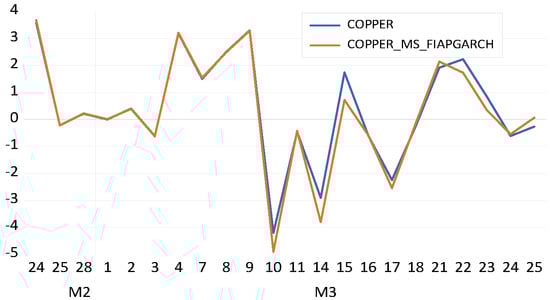
Figure 2.
Copper, MS−FIAPGARCH.
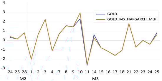
Figure 3.
Gold, MS−FIAPGARCH−MLP.
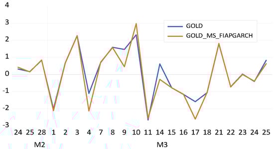
Figure 4.
Gold, MS−FIAPGARCH.

Figure 5.
Oil, MS−FIAPGARCH−MLP.
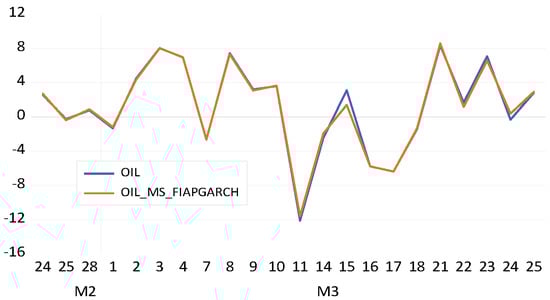
Figure 6.
Oil, MS−FIAPGARCH.
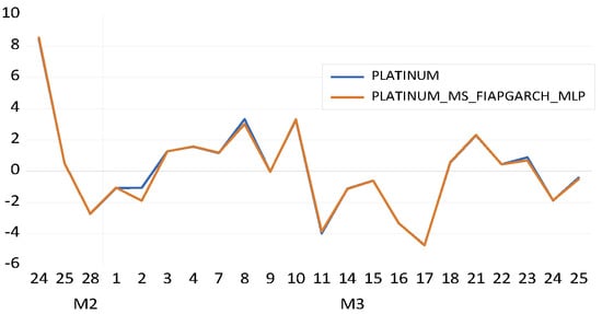
Figure 7.
Platinum, MS−FIAPGARCH−MLP.
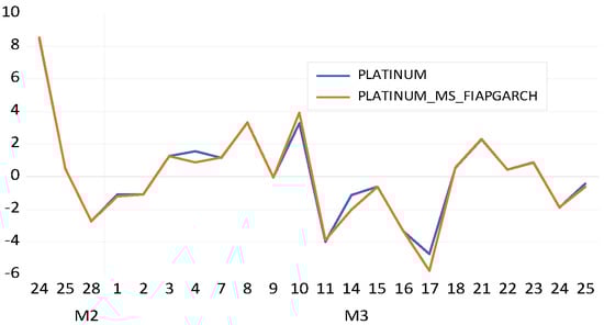
Figure 8.
Platinum, MS−FIAPGARCH.
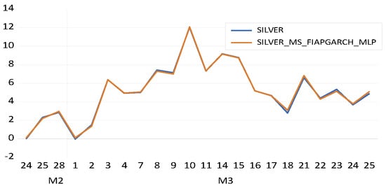
Figure 9.
Silver, MS−FIAPGARCH−MLP.
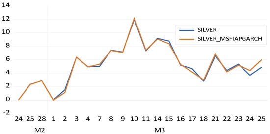
Figure 10.
Silver, MS−FIAPGARCH.
4.3. Discussion and Policy Recommendations
The results can be provided in three subgroups, a. the MSFIAPGARCH and MSFIAPGARCH–MLP–copula methods are suitable to determine contagion effect and the persistence, b. the effects of the returns of the precious metals are significantly higher than the effects of oil prices. So, the results suggest that the returns of precious metals can be more sensitive than the volatility in the oil price, c. the normality assumption is not suitable for making neither financial nor economic decisions and. there are persistence, dependence and contagion between the variables.
The empirical results provided important insights regarding the relations between the oil and the selected precious metals in terms of regime–dependent contagion and dependence structure. The augmented copula models captured two distinct regimes characterized as low–volatility and high–volatility regimes. The long memory characteristics are observed in both regimes suggesting persistence in all series analyzed. Further, the MLP–augmented variants achieved significant level of improvement for precious metals’ return predictability. Further, results also favored significance of leverage effects suggesting asymmetric response of the series to negative compared to positive shocks and news.
The results found some important points. Therefore, it was determined a higher dependence structure between the returns of the precious metals and oil price during R1 period than during the R2 ones. The results mean the dependence structures between oil price volatilities and precious metals returns are deeper than the other one. The results recommend the existence of a contagion effect and indicated that diversification can be less effective and that determining a portfolio that covers precious metals and oil during high–volatility regimes and/or the crisis period is a theme to systematic risk.
Similar to the results of Wen [83], Zhu [76], and Aloui [62], the findings determined the evidence of a dependence structure between the analyzed variables. Further, the findings also confirmed the validity of the works Boubaker and Shaier [29,64,65] and Bildirici [30,54,69,75]. The dependence structure changes between regimes. This effect shows that severe changes in energy prices impact precious metals prices. The energy risk managers and the investors who embrace oil as an asset in a differentiated portfolio must considerdownside risk disclosure and must accentuate the leftside of the return distribution of portfolio. Therefore, the results obtained by this paper lead to important policy implications for the governments, policymakers, portfolio managers and investors. The volatility of oil, in addition to that of precious metals, is subject to persistence that should be taken into consideration during policy and investment decisions. Further, such long memory characteristics, especially for oil, also should be kept in consideration by the central banks that aim at controlling inflationary policies. Since price instabilities of oil have important impacts on the inflation, the governments should aim at the minimization of volatility of oil and precious metal prices. The volatilities of oil price impact the persistence of inflation, and moreover can trigger the rise in asset prices due to leading to inflationary pressures. These results can also lead to important insights for the investors. Within an international and national investor perspective, individuals and institutions and portfolio managers have to consider the behavior of copper and silver in their precious metal portfolios because its low correlation makes it a good hedge asset in addition to considering the high levels of contagion between oil and all precious metals analyzed.
The findings obtained in this study highlighted that the analyzed precious metal and oil price volatilities are subject to fractionally integrated characteristics which are regime–dependent. The MS–FIAPGARCH and MSFIAPGARCH–MLP models in this study allow the modeling of such marginal distributions with processes which will be used to be utilized to obtain regime dependent tail dependence that provides important insights for investors and policy makers. It should also be stated that the fractional integration characteristics and chaotic behavior in the analyzed series require caution. Therefore, though important improvement in forecasts is achieved, modeling series with such characteristics can also lead to important limitations. The chaotic structure in the precious metal and oil prices show that, under drastic changes in economic policies or unexpected shocks, the series would lead to strong deviations from the analyzed relationships and forecasted values. Under these circumstances, the investors should be aware of such limitations of the proposed models similar to many time series models. The recent COVID-19 pandemic led to strong deviations of oil prices in addition to precious metals. Due to the lockdown and the shocks caused by the pandemic, the period of COVID-19 has been subject to strong fluctuations in industrial production and significant changes in the investor behavior not to mention the fluctuations in risk and return relationship. Given the chaotic, fractional integration and persistence characteristics of precious metals and oil prices, the forecast performances of our models would deteriorate if the forecast experiment had been conducted for the early days of pandemic. However, such conclusions cannot be drawn without testing and simulating such an experiment which is left for future studies.
However, it should be noted that the models provide forecast improvement under such turbulent periods. The sample period is between 1 January 1990 and 25 March 2022 and the out–of–sample forecasting evaluation is conducted for the last 30 days covering the early days of March 2022 which provided an interesting experiment for our models. The Ukraine–Russia War started on 20 February 2022 and had important effects on the world economies, not to mention the energy crisis and fluctuations in oil prices. During the period, precious metals have also been subject strong fluctuations. As seen in Table 8, MSE and RMSE results provided significant improvement in forecast performances for out–of–sample forecasts that covers the Russia–Ukraine war. If models are compared in this respect, the MLP–type neural network–augmented MS–FIAPGARCH–MLP model showed significant gains in forecast performance over its non–MLP–augmented counterpart for all precious metals and oil series analyzed. The results show that MLP–based neural networks augmentations provide improvement in forecasting in such turbulent periods. The augmentation of the proposed models with deep neural networks would provide a new area of research for the future studies.
5. Conclusions
This study determines the predictability of oil, gold, copper, silver, platinum through the MS–FIAPGARCH–copula and MS–FIAPGARCH–MLP–copula methods for the 1 January 1990–25 March 2022 period. The MS–FIAPGARCH–copula model allows the investigation of nonlinearity and asymmetry in capturing regime–specific fractional integration and long memory characteristics and asymmetric power structures for the conditional variance processes in addition to allowing the assessment of regime–specific dependence between the analyzed series. The MS–FIAPGARCH–MLP model further augments the MS–FIAPGARCH model with MLP–type neural networks to augment the forecast capabilities. The results obtained by this paper led to important policy implications. The nonlinearity and regime dependent volatility in addition to asymmetric dependence and contagion relations cannot be rejected for policy makers and investors. The long memory characteristics, especially for oil, also should be kept in consideration also by the central banks focusing on anti–inflationary policies. The price volatility in oil in addition to precious metals are known to affect persistence of inflation which in turn led to increasing policy interest rates that affect financial markets especially stock markets. Results also favored addition of copper and silver in the precious metal portfolios for its hedge asset characteristics in addition to keeping in mind the high contagion between oil and the precious metals.
Author Contributions
Conceptualization, M.B. and Ö.Ö.E.; methodology, M.B. and Ö.Ö.E.; software, M.B. and Ö.Ö.E.; validation, M.B. and Ö.Ö.E.; formal analysis, M.B. and Ö.Ö.E.; investigation, M.B. and Ö.Ö.E.; resources, M.B. and Ö.Ö.E.; data curation, M.B. and Ö.Ö.E.; writing—original draft preparation, M.B. and Ö.Ö.E.; writing—review and editing, M.B. and Ö.Ö.E.; visualization, M.B. and Ö.Ö.E.; supervision, M.B.; project administration, M.B. and Ö.Ö.E.; funding acquisition, M.B. and Ö.Ö.E. All authors have read and agreed to the published version of the manuscript.
Funding
This research received no external funding.
Data Availability Statement
Data is available from Bloomberg database and from the corresponding author upon request.
Conflicts of Interest
The authors declare no conflict of interest.
References
- U.S. Geological Survey. USGS Minerals Yearbook 2014, 1st ed.; National Minerals Information Center: Reston, VA, USA. Available online: https://minerals.usgs.gov/minerals/pubs/commodity/tin/myb1-2014-tin.pdf (accessed on 18 November 2022).
- Bildirici, M.E.; Turkmen, C. Nonlinear causality between oil and precious metals. Resour. Policy 2015, 46, 202–211. [Google Scholar] [CrossRef]
- Arouri, M.; Hammoudeh, S.; Lahiani, A.; Nguyen, D. Long memory and structural breaks in modelling the return and volatility dynamics of precious metals. Q. Rev. Econ. Financ. 2012, 52, 207–218. [Google Scholar] [CrossRef]
- Bildirici, M.; Ozaksoy, F. The effects of oil and gold prices on oil-exporting countries. Energy Strategy Rev. 2018, 22, 290–302. [Google Scholar] [CrossRef]
- Gil-Alana, L.A.; Tripathy, T. Modelling volatility persistence and asymmetry: A Study on selected Indian non-ferrous metals markets. Resour. Policy 2014, 41, 31–39. [Google Scholar] [CrossRef]
- Bildirici, M.; Ersin, Ö. Forecasting oil prices: Smooth transition and neural network augmented GARCH family models. J. Pet. Sci. Eng. 2013, 109, 230–240. [Google Scholar] [CrossRef]
- Bildirici, M.; Ersin, Ö. Modeling Markov switching ARMA-GARCH neural networks models and an application to forecasting stock returns. Sci. World J. 2014, 497941. [Google Scholar] [CrossRef]
- Bildirici, M.; Ersin, Ö. Forecasting volatility in oil prices with a class of nonlinear volatility models: Smooth transition RBF and MLP neural networks augmented GARCH approach. Pet. Sci. 2015, 12, 534–552. [Google Scholar] [CrossRef]
- Bildirici, M.; Ersin, Ö. Markov switching artificial neural networks for modelling and forecasting volatility: An application to gold market. Procedia Econ. Finance 2016, 38, 106–121. [Google Scholar] [CrossRef]
- Ersin, Ö.; Bildirici, M. Markov-switching vector autoregressive neural networks and sensitivity analysis of environment, economic growth and petrol prices. Environ. Sci. and Pol. Res. 2018, 25, 31630–31655. [Google Scholar]
- Hamilton, J.D. Analysis of time series subject to changes in regime. J. Econ. 1990, 45, 39–70. [Google Scholar] [CrossRef]
- Cuddington, J.; Jerrett, D. Super cycles in real metals prices? IMF Staff. Pap. 2008, 55, 541–565. [Google Scholar] [CrossRef]
- U.S. Geological Survey USGS. Mineral Commodity Summaries 2012, 1st ed.; National Minerals Information Center: Reston, VA, USA, 2012. [Google Scholar] [CrossRef]
- Wilburn, D.; Bleiwas, D.I. Platinum-Group Metals—World Supply and Demand, Open-File Report 2004, Series Number 1224. Available online: https://pubs.er.usgs.gov/publication/ofr20041224 (accessed on 18 November 2022).
- Hansen, B. Rethinking the univariate approach to unit root testing-using covariates to increase power. Econ. Theory 1995, 11, 1148–1171. [Google Scholar] [CrossRef]
- Stock, J.H. Unit roots, structural breaks and trends. In Handbook of Econometrics, 1st ed.; Engle, R.F., McFadden, D.L., Eds.; Elsevier: Amsterdam, The Netherlands, 1994; Chapter 46; pp. 2379–2841. [Google Scholar]
- Gil-Alana, L.A.; Chang, S.; Balcilar, M.; Aye, G.C.; Gupta, R. Persistence of precious metal prices: A fractional integration approach with structural breaks. Resour. Policy 2015, 44, 57–64. [Google Scholar] [CrossRef]
- Lee, J.; List, J.A.; Strazicich, M.C. Non-renewable resource prices: Deterministic or stochastic trends? J. Environ. Econ. Manag. 2006, 51, 354–370. [Google Scholar] [CrossRef]
- Carnero, M.A.; Peña, D.; Ruiz, E. Effects of outliers on the identification and estimation of GARCH models. J. Time Ser. Anal. 2007, 28, 471–497. [Google Scholar] [CrossRef]
- Carnero, M.A.; Peña, D.; Ruiz, E. Estimating GARCH volatility in the presence of outliers. Econ. Lett. 2012, 114, 86–90. [Google Scholar] [CrossRef][Green Version]
- Aggarwal, R.; Inclan, C.; Leal, R. Volatility in emerging markets. J. Financial Quant. Anal. 1999, 34, 33–55. [Google Scholar] [CrossRef]
- Charles, A. Forecasting volatility with outliers in GARCH models. J. Forecast. 2008, 27, 551–565. [Google Scholar] [CrossRef]
- Ané, T.; Loredana, U.R.; Gambet, J.B.; Bouverot, J. Robust outlier detection for Asia-Pacific stock index returns. Int. Finance Mark. Inst. Money 2008, 18, 326–343. [Google Scholar] [CrossRef]
- Charles, A.; Darné, O. Volatility persistence in crude oil markets. Energy Policy 2014, 65, 729–742. [Google Scholar] [CrossRef]
- Charles, A.; Darné, O. Large shocks in the volatility of the dow jones industrial average index: 1928–2013. J. Bank. Finance 2014, 43, 188–199. [Google Scholar] [CrossRef]
- Laurent, S.; Lecourt, C.; Palm, F.C. Testing for jumps in conditionally gaussian ARMA-GARCH models, a robust approach. Comput. Stat. Data Anal. 2016, 100, 383–400. [Google Scholar] [CrossRef]
- Chan-Lau, J.A.; Mathieson, D.J.; Yao, J.Y. Extreme contagion in equity markets. IMF Staff. Pap. 2004, 51, 386–408. [Google Scholar] [CrossRef]
- Forbes, K.J.; Rigobon, R. No contagion, only interdependence: Measuring stock market comovements. J. Finance 2002, 57, 2223–2261. [Google Scholar] [CrossRef]
- Boubaker, H.; Sghaier, N. Instability and dependence structure between oil prices and GCC stock markets. Energy Stud. Rev. 2014, 20, 50–65. [Google Scholar] [CrossRef][Green Version]
- Bildirici, M. The chaotic behavior among the oil prices, expectation of investors and stock returns: TAR-TR-GARCH copula and TAR-TR-TGARCH copula. Pet. Sci. 2019, 16, 217–228. [Google Scholar] [CrossRef]
- McKenzie, M.; Mitchell, H.; Brooks, R.; Faff, R. Power ARCH modeling of commodity futures data on the London metal exchange. Eur. J. Finance 2001, 7, 22–38. [Google Scholar] [CrossRef]
- Lin, L.; Kuang, Y.; Jiang, Y.; Su, Z. Assessing risk contagion among the Brent crude oil market, London gold market and stock markets: Evidence based on a new wavelet decomposition approach. N. Am. J. Econ. Fin. 2019, 50, 101035. [Google Scholar] [CrossRef]
- Tully, E.; Lucey, B.M. A power GARCH examination of the gold market. Res. Int. Bus. Finance 2007, 21, 316–325. [Google Scholar] [CrossRef]
- Kang, S.H.; Kang, S.M.; Yoon, S.M. Forecasting volatility of crude oil markets. Energy Econ. 2009, 31, 119–125. [Google Scholar] [CrossRef]
- Morales, L.; Andreosso-O’Callaghan, B. Comparative analysis on the effects of the Asian and global financial crises on precious metals markets. Res. Int. Bus. Finance 2011, 25, 203–227. [Google Scholar] [CrossRef]
- Cochran, S.J.; Mansur, I.; Odusami, B. Threshold Effects of the Term Premium in 25 Metal Returns and Return Volatilities: A Double Threshold-FIGARCH Approach; Working Paper; Villanova University: Villanova, PA, USA, 2011; pp. 1–30. [Google Scholar]
- Cochran, S.J.; Mansur, I.; Odusami, B. Volatility persistence in metal returns: A FIGARCH approach. J. Econ. Bus. 2012, 64, 287–305. [Google Scholar] [CrossRef]
- Ewing, B.; Malik, F. Volatility transmission between gold and oil futures under structural breaks. Int. Rev. Econ. Finance 2013, 25, 113–121. [Google Scholar] [CrossRef]
- Chkili, W.; Hammoudeh, S.; Nguyen, D.K. Volatility forecasting and risk management for commodity markets in the presence of asymmetry and long memory. Energy Econ. 2014, 4, 1–18. [Google Scholar] [CrossRef]
- Tiwari, A.K.; Sahadudheen, I. Understanding the nexus between oil and gold. Resour. Policy 2015, 46, 85–91. [Google Scholar] [CrossRef]
- Behmiri, N.B.; Manera, M. The role of outliers and oil price shocks on volatility of metal prices. Resour. Policy 2015, 46, 139–150. [Google Scholar] [CrossRef]
- Mensi, W.; Nekhili, R.; Vo, X.V.; Kang, S.H. Oil and precious metals: Volatility transmission, hedging, and safe haven analysis from the Asian crisis to the COVID-19 crisis. Econ. Anal. Policy 2021, 71, 73–96. [Google Scholar] [CrossRef]
- Hammoudeh, S.; Yuan, Y. Metal volatility in presence of oil and interest rate shocks. Energy Econ. 2008, 30, 606–620. [Google Scholar] [CrossRef]
- Diaz, F.J. Do scarce precious metals equate to safe harbor investments? The case of platinum and palladium. Econ. Res. Int. 2016, 2361954. [Google Scholar] [CrossRef]
- Das, D.; Bhatia, V.; Kumar, S.B.; Basu, S. Do precious metals hedge crude oil volatility jumps? Int. Rev. Finance Anal. 2022, 83, 102257. [Google Scholar] [CrossRef]
- Ahmed, R.; Chaudhry, S.; Kumpamool, C.; Benjasak, C. Tail risk, systemic risk and spillover risk of crude oil and precious metals. Energy Econ. 2022, 112, 106063. [Google Scholar] [CrossRef]
- Bentes, S.R. On the stylized facts of precious metals’ volatility: A comparative analysis of pre- and during COVID-19 crisis. Phys. A 2022, 600, 127528. [Google Scholar] [CrossRef]
- Dinh, T.; Goutte, S.; Nguyen, D.K.; Walther, T. Economic drivers of volatility and correlation in precious metal markets. J. Commod. Mark. 2022, 100242. [Google Scholar] [CrossRef]
- Mensi, W.; Ali, S.; Vo, X.; Kang, S. Multiscale dependence, spillovers, and connectedness between precious metals and currency markets: A hedge and safe-haven analysis. Resour. Policy 2022, 77, 102752. [Google Scholar] [CrossRef]
- Sephton, P.S. Revisiting the inflation-hedging properties of precious metals in Africa. Resour. Policy 2022, 77, 102735. [Google Scholar] [CrossRef]
- Kaczmarek, T.; Będowska-Sojka, B.; Grobelny, P. False safe haven assets: Evidence from the target volatility strategy based on recurrent neural network. Res. Int. Bus. Finance 2022, 60, 101610. [Google Scholar] [CrossRef]
- Jahanshahi, H.; Yousefpour, A.; Wei, Z.; Alcaraz, R.; Bekiros, S. A financial hyperchaotic system with coexisting attractors: Dynamic investigation, entropy analysis, control and synchronization. Chaos Solitons Fractals 2019, 126, 66–77. [Google Scholar] [CrossRef]
- Bildirici, M.; Sonüstün, F.O. Chaotic behavior in gold, silver, copper and bitcoin prices. Resour. Policy 2021, 74, 102386. [Google Scholar] [CrossRef]
- Bildirici, M.E. Chaos structure and contagion behavior between COVID-19, and the returns of prices of precious metals and oil: MS-GARCH-MLP copula. Nonlinear Dyn. Psychol. Life Sci. 2022, 26, 209–219. [Google Scholar]
- Syllignakis, M.N.; Kouretas, G.P. Dynamic correlation analysis of financial contagion: Evidence from the central and eastern European markets. Int. Rev. Econ. Finance 2011, 20, 717–732. [Google Scholar] [CrossRef]
- Choe, K.I.; Choi, P.; Nam, K.; Vahid, F. Testing financial contagion on heteroskedastic asset returns in time-varying conditional correlation. Pacific-Basin Finance J. 2012, 20, 271–291. [Google Scholar] [CrossRef]
- Celik, S. The more contagion effect on emerging markets: The evidence of DCC-GARCH model. Econ. Model. 2012, 29, 1946–1959. [Google Scholar] [CrossRef]
- Ahmad, W.; Sehgal, S.; Bhanumurthy, N.R. Eurozone crisis and BRIICKS stock markets: Contagion or market interdependence? Econ. Model. 2013, 33, 209–225. [Google Scholar] [CrossRef]
- Pesaran, B.; Pesaran, M.H. Conditional volatility and correlations of weekly returns and the VaR analysis of 2008 stock market crash. Econ. Model. 2010, 27, 1398–1416. [Google Scholar] [CrossRef]
- Guo, F.; Chen, C.R.; Huang, Y.S. Markets contagion during financial crisis: A regime switching approach. Int. Rev. Econ. Finance 2011, 20, 95–109. [Google Scholar] [CrossRef]
- Ramchand, L.; Susmel, R. Volatility and cross correlation across major stock markets. J. Empir. Finance 1998, 5, 397–416. [Google Scholar] [CrossRef]
- Aloui, R.; Ben-Aissa, M.S.; Nguyen, D.K. Global financial crisis, extreme interdependences and contagion effects: The role of economic structure? J. Bank. Finance 2011, 35, 130–141. [Google Scholar] [CrossRef]
- Rodriguez, J.C. Measuring financial contagion: A copula approach. J. Empir. Finance 2007, 14, 401–423. [Google Scholar] [CrossRef]
- Boubaker, H.; Sghaier, N. Contagion effect and change in the dependence between oil and ten MENA stock markets. RRJSMS 2016, 2, 1–17. [Google Scholar]
- Boubaker, H.; Sghaier, N. Markov-switching time-varying copula modeling of dependence structure between oil and GCC stock markets. Open J. Stat. 2016, 6, 565–589. [Google Scholar] [CrossRef]
- Francq, C.; Zakoian, J. Stationarity of multivariate Markov-switching ARMA models. J. Econ. 2001, 102, 339–364. [Google Scholar] [CrossRef]
- Henneke, S.; Rachev, S.; Fabozzi, F.; Nikolov, M. MCMC-based Estimation of Markov Switching ARMA-GARCH Models. Appl. Econ. 2011, 43, 259–271. [Google Scholar] [CrossRef]
- Joe, H. Multivariate Models and Dependence Concepts, 1st ed.; Chapman & Hall: London, UK, 1997; pp. 1–416. [Google Scholar]
- Bildirici, M.; Salman, M.; Ersin, Ö. Nonlinear contagion and causality nexus between oil, gold, VIX investor sentiment, exchange rate and stock market returns: The MS-GARCH copula causality method. Mathematics 2022, 10, 4035. [Google Scholar] [CrossRef]
- Reboredo, J.; Rivera-Castro, M.A. A wavelet decomposition approach to crude oil price and exchange rate dependence. Econ. Model. 2013, 32, 42–57. [Google Scholar] [CrossRef]
- Tsay, R.S. Nonlinearity tests for time series. Biometrika 1986, 73, 461–466. [Google Scholar] [CrossRef]
- Hsieh, D. Chaos and nonlinear dynamics: Application to financial markets. J. Finance 1991, 46, 1839–1877. [Google Scholar] [CrossRef]
- Eckmann, J.P.; Ruelle, D. Ergodic theory of chaos and strange attractors. Theory Chaotic Attractors 1985, 57, 617. [Google Scholar]
- Adrangi, B.; Chatrath, A.; Dhanda, K.K.; Raffiee, K. Chaos in oil prices? Evidence from futures markets Energy Econ. 2001, 23, 405–425. [Google Scholar]
- Bildirici, M.; Sonüstün, F.O. Chaotic structure of oil prices. AIP Conf. Proc. 2018, 1926, 20009. [Google Scholar]
- Zhu, H.M.; Li, R.; Li, S. Modelling dynamic dependence between crude oil prices and asia-pacific stock market returns. Int. Rev. Econ. Finance 2013, 29, 208–223. [Google Scholar] [CrossRef]
- Cashin, P.; McDermott, C.; Scott, A. Booms and slumps in world commodity prices. J. Dev. Econ. 2002, 69, 277–296. [Google Scholar] [CrossRef]
- Rossen, A. What are metal prices like? Co-movement, price cycles and long-run trends. Resour. Policy 2015, 45, 255–276. [Google Scholar] [CrossRef]
- Masa, A.; Diaz, F.J. Long-memory modelling and forecasting of the returns and volatility of exchange-traded notes (ETNs). J. Appl. Econ. Res. 2017, 11, 23–53. [Google Scholar] [CrossRef]
- Batten, J.A.; Ciner, C.; Lucey, B.M. The macroeconomic determinants of volatility in precious metals markets. Resour. Policy 2010, 35, 65–71. [Google Scholar] [CrossRef]
- Fassas, A. Exchange-traded products investing and precious metal prices. J. Deriv. Hedge Funds 2012, 18, 127–140. [Google Scholar] [CrossRef]
- Sensoy, A. Dynamic relationship between precious metals. Resour. Policy 2013, 38, 504–511. [Google Scholar] [CrossRef]
- Wen, X.; Wei, Y.; Huang, D. Measuring contagion between energy market and stock market during financial crisis: A copula approach. Energy Econ. 2012, 34, 1435–1446. [Google Scholar] [CrossRef]
- Donaldson, R.G.; Kamstra, M. An artificial neural network—GARCH model for international stock return volatility. J. Empir. Finance 1997, 4, 17–46. [Google Scholar] [CrossRef]


Publisher’s Note: MDPI stays neutral with regard to jurisdictional claims in published maps and institutional affiliations. |
© 2022 by the authors. Licensee MDPI, Basel, Switzerland. This article is an open access article distributed under the terms and conditions of the Creative Commons Attribution (CC BY) license (https://creativecommons.org/licenses/by/4.0/).