Article

Representation Learning with a Variational Autoencoder for Predicting Nitrogen Requirement in Rice

Ecodevelopment S.A., Filyro P.O. Box 2420, 57010 Thessaloniki, Greece
*
Author to whom correspondence should be addressed.
Remote Sens. 2022, 14(23), 5978; https://doi.org/10.3390/rs14235978
Submission received: 7 October 2022 / Revised: 11 November 2022 / Accepted: 22 November 2022 / Published: 25 November 2022
(This article belongs to the Special Issue Remote Sensing of Agro-Ecosystems)

Abstract

:
The scope of this research was to provide rice growers with optimal N-rate recommendations through precision agriculture applications. To achieve this goal, a prediction rice yield model was constructed, based on soil data, remote sensing data (optical and radar), climatic data, and farming practices. The dataset was collected from a rice crop surface of 89.2 ha cultivated continuously for a 5-year period and was analyzed with machine learning (ML) systems. A variational autoencoder (VAE) for reconstructing the input data of the prediction model was applied, resulting in MAE of 0.6 tn/ha, with an average yield for the study fields and period measured at 9.6 tn/ha. VAE learns the original input data representation and transforms them in a latent feature space, so that the anomalies and the discrepancies of the data are reduced. The reconstructed data by VAE provided a more sophisticated and detailed ML model, improving our knowledge about the various correlations between soil, N management parameters, and yield. Both optical and radar imagery and the climatic data were found to be of high importance for the model, as indicated by the application of XAI (explainable artificial intelligence) techniques. The new model was applied in the 2022 rice cultivation in the study fields, resulting in an average yield increase of 4.32% compared to the 5 previous years of experimentation.

Graphical Abstract

1. Introduction

Nitrogen (N) is the most significant macronutrient for rice growing, limiting yield when not supplied in sufficiency [1]. However, if the rice crop is oversupplied with N, then expenses for N fertilization, rice lodging risk, and N losses to the environment increase [2]. On the other hand, growers are reluctant to fertilize with low N doses, because if the yield is reduced, then the economic saving due to the reduced cost of N fertilization cannot compensate for the economic losses caused by yield reduction [3].
The progress of machine learning (ML) allows for recognizing patterns within the data to automatically predict future events or aid in decision making [4,5]. As ML algorithms can capture nonlinear relationships within data, they can uncover complex data structures, which normally characterize the environmental data and make predictions based on knowledge gained from the data. The progress—in parallel—of remote sensing and the increased availability of data coming from satellites provides a wealth of useful information that is difficult to model using the commonly known statistical methods [6].
Rice growth simulation models, such as RiceGrow, ORYZA2000, SIMRIW, and CERES-Rice, have been used for predicting the phenology and organ biomass of rice in relation to environmental parameters [7,8,9,10]. However, these models are difficult to use under operational conditions because they require data that cannot be recorded by the growers [11]. Plant growth models are important for validating scientific hypotheses or plant processes observed in a laboratory through experimentation. The scope of crop growth models is to predict, among other things, canopy growth based on varying a particular factor, such as N. This can confirm scientific hypotheses or data collected in a laboratory, but as mentioned above, it is difficult to use under commercial conditions for making assumptions for fertilizer recommendations. As crop models have high requirements for data that are difficult to obtain under operational conditions, often crop models cannot respond as expected to the environmental factors. However, due to their mechanistic nature, crop growth models are useful for research purposes, as testing parts of the model can result in improvement of the final error in growth predictions and provide better understanding of the factors affecting plant growth [12]. Nonetheless, data-driven prediction models using open-source remote sensing data seem to be a more viable option in operational farming practice.
There is currently a trend to predict crop yield late in the season (close to harvest) to enable growers to diagnose crop conditions and adopt necessary measures for the next season. Jeong et al. [13] showed that a long–short memory (LSTM) network along with a one-dimensional convolutional layer (1D-CNN) had good performance (R2 = 0.859) for predicting yield two months before rice yield. However, this prediction cannot provide information for the current season’s N fertilization, as N topdressing fertilization in rice is done 3 months before harvest. Moreover, N optimal dose is affected by current weather conditions and plant growth and cannot be estimated based solely on soil data or management practices. However, these models are useful for enabling better management of food supplies and food security.
In early 2021, Iatrou et al. [2] published a model on topdressing fertilization of rice in Greece using machine learning techniques. The model included meteorological data of the critical period from seeding to pre-booting (normally, early July), but did not incorporate similar data of the postfertilization period (as the main intension was to predict immediate topdressing fertilization needs). After less than a month, however, exceptionally high temperatures hit the area of the Thessaloniki Plain for 10 consecutive days, affecting seriously rice fertility rates and consequently lowering the yield three months later. That was a great lesson, showing the necessity to include meteorological data of the flowering season too, in predicting topdressing fertilization needs based on weather particularities of the entire cultivation season and not only the “before” period. In the case of high temperatures, the fertilization rates should be higher than normal and vice versa. This is because high N levels contribute to higher numbers of panicles, spikelets per panicle, and grain weight alleviating the effect of high temperatures on rice production [14].
Environmental data, such as temperature and precipitation, earth observation data, and soil data, can have high variance within a field or from field to field and from year to year. This variance can affect the output of an ML yield prediction algorithm, as the ML algorithm learns how each variable correlates with high or low yield. To deal with the problem of making an ML that superficially understands the data, i.e., learning from events that occurred in the continuous series of events that took place during experimentation, representation learning should be adopted. Representation learning provides the ML algorithm with a more abstract representation of the data so that the anomalies and the discrepancies of the data are reduced. Thus, variational autoencoders can be used that provide latent variables of the initial input variables that are a lower order representation of the initial data. In practice, the autoencoders are models designed to capture the underlying distribution of the input data and replicate the original data to another level. This level did not exist in the original data, but it could have existed based on the underlying patterns in the original data [15].
The scope of this research was to develop a decision support tool for providing rice growers with sound N fertilizer recommendations in the framework of precision agriculture applications. Precision agriculture (or precision farming) is a management strategy considering within-field crop variability towards improved resource use efficiency, productivity, quality, profitability, and sustainability of agricultural production [16,17].
To achieve the research aims, a rice yield prediction model was constructed using machine learning (ML) systems, based on soil and climatic data, remote sensing indices and farming practices (including day of seeding and cultivar) collected from extended surfaces cultivated intensively with rice for a continuous 5-year period (2017–2021).

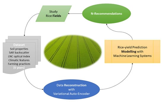
2. Materials and Methods
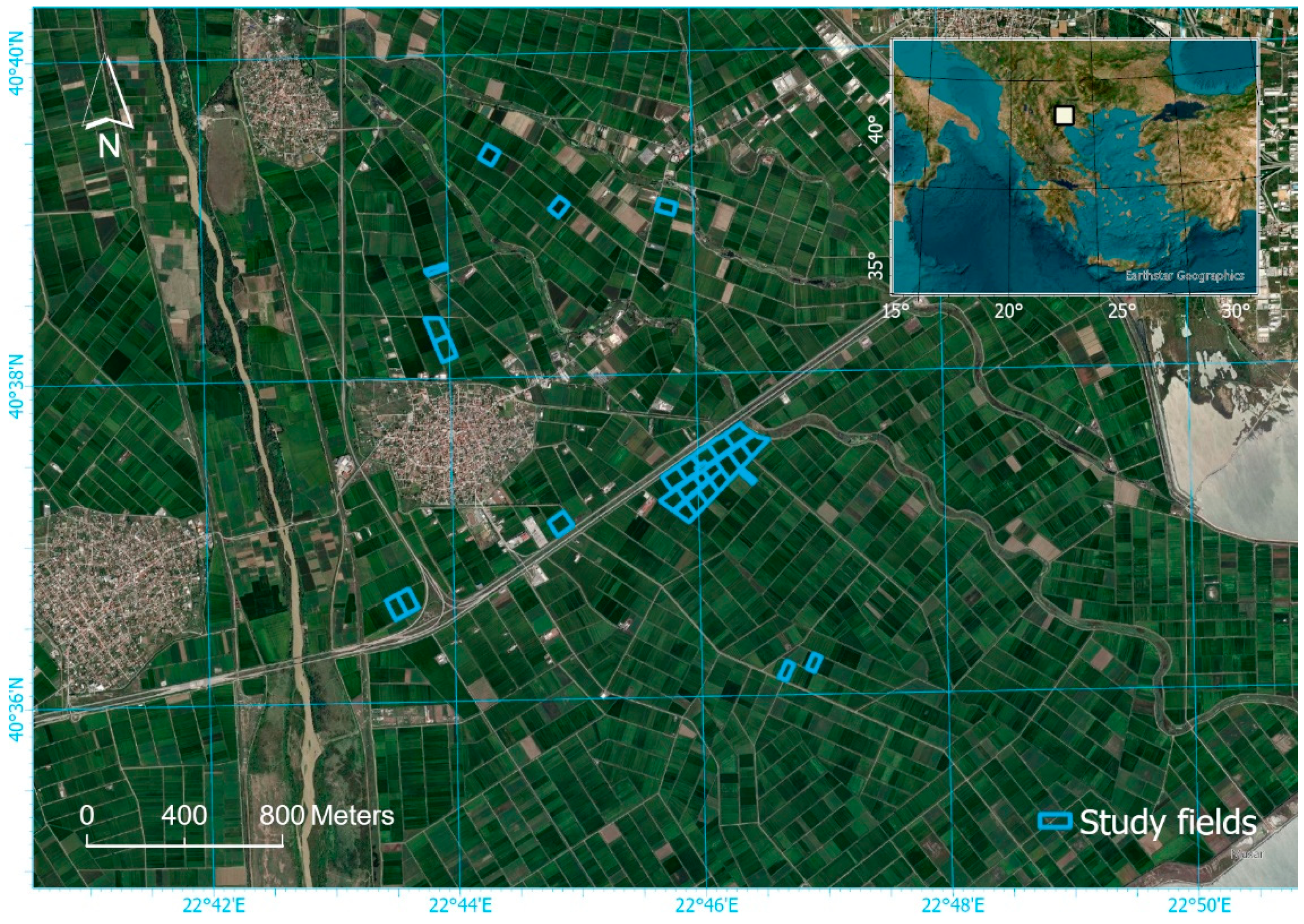
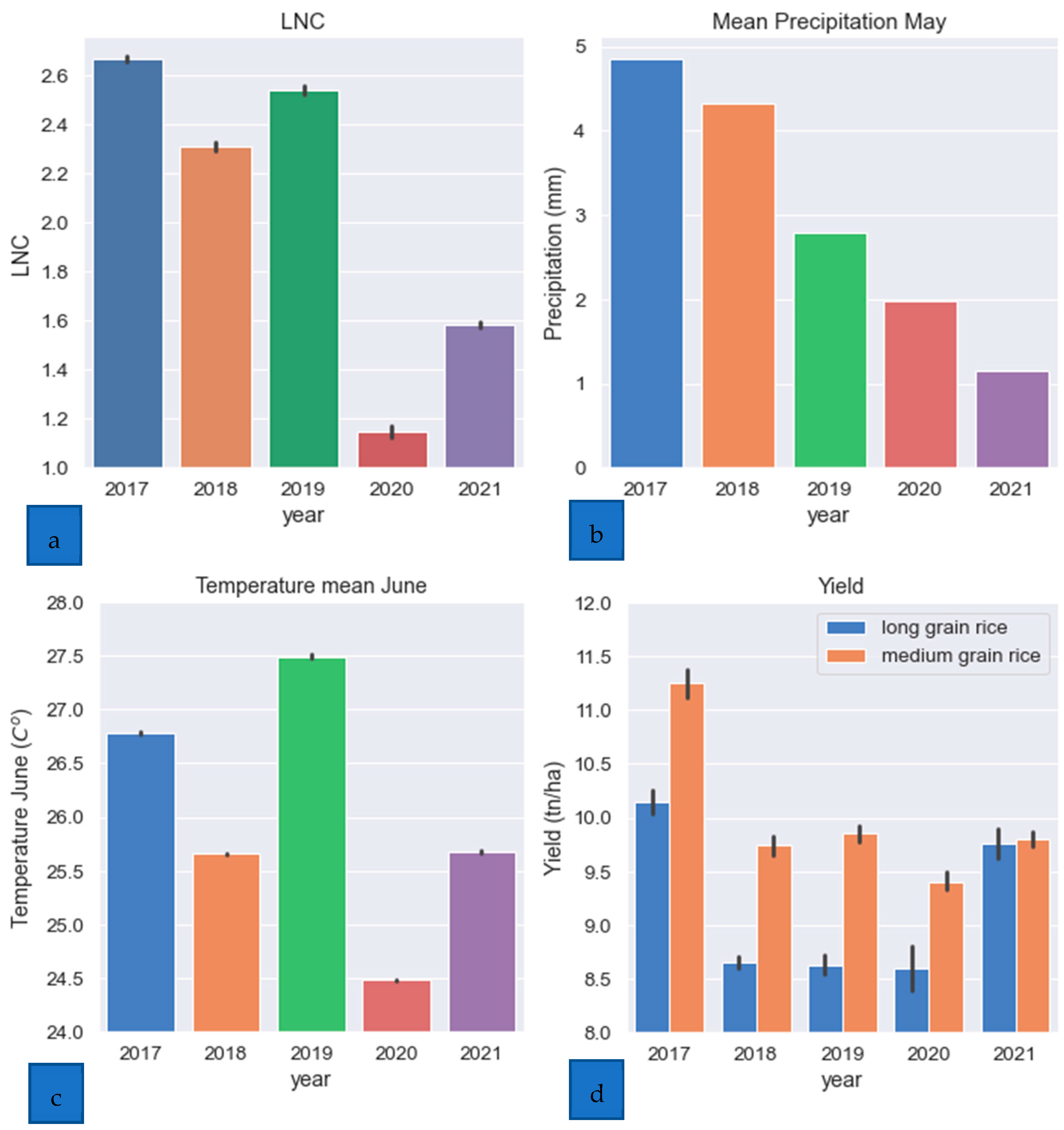
2.1. Study Area

The study area is in the Thessaloniki Plain, Greece, a low-lying coastal area of about 22,400 ha and the main rice production zone of Greece. The climate of the area is typical Mediterranean, with temperate summers suitable for rice cultivation, even for genotypes of indica type. Rice is the main crop in the area, about 75%, and rotated with maize, cotton, and alfalfa.
The alluvial soils of the plain are mostly silty clay, poorly drained, and classified as typic xerofluvents. However, salinity levels remain too low to imply any soil degradation hazard, according to recent experiments conducted by Litskas et al. [18].
Sowing is carried out in mid-May, while harvesting is carried out in October, depending on grain moisture levels (which must ideally be from 19% to 21%). The plain produces the highest recorded yield (almost 10 ton/ha on average) among all the rice producing plains in Greece (8.89 ton/ha on average).
A surface of 89.2 ha comprising part of the rice farm of Mr. Kostas Kravvas and located around the rural town of Chalastra (40.6265°N, 22.7307°E, 6 m altitude) was selected for the study. The selected fields were continuously cultivated with rice with precision agriculture methodologies for the studied period, i.e., from 2017 to 2021. The mean extent of the studied fields was 3.18 ha (Figure 1).

2.2. Dataset Preparation

A multisource dataset covering the study fields was collected for five continuous cultivation seasons (2017–2021). The nature of the original data can be distinguished into soil properties, climatic measurements, farming practices, crop spectral properties, and yield.
  • Soil properties
Soil properties are of particular importance to fertilization recommendations [19]. Soil properties in this research were derived from original soil sampling surveys in the studied rice fields conducted in 2016 (61 samples), 2018 (40 samples), and 2020 (111 samples) (totally, 212 samples). In 2016 and 2018, the sampling design followed a site-specific scheme according to the crop heterogeneity patterns detected in satellite image time series [19]; in 2020, the sampling design followed a 90 × 90 m regular grid. The site-specific design (2016, 2018) resulted in a density of one sample per 0.88 hectares, while the regular design (2020) resulted in one sample per 0.80 hectares; thus, both surveys resulted in similar densities.
Cylindrical soil columns 30 cm deep were extracted from naked soil surfaces in winter at each sampling point and sent for full analysis to the Soil and Water Resource Institute, Hellenic Agricultural Organization (DEMETER). The samples underwent full analysis for a set of 18 soil properties: weight percentage of sand, clay, and silt, bulk density, soil acidity (pH), electrical conductivity (EC), organic matter (OM), CaCO3, nitrate nitrogen, phosphorus, potassium, magnesium, iron, zinc, manganese, copper, boron, and calcium [20].
Finally, the point sample map was converted into raster surfaces for all measured soil properties using the inverse distance weighting (IDW) spatial interpolation method, thus resulting in a set of 18 soil surfaces.
b.
Climatic measurements
Surface temperature influences the growth stage during the whole growing season. The combined thermal condition of the atmosphere within the planetary boundary layer is connected to the parameter of land surface temperature (LST). The MODIS sensor was used to retrieve the LST during the day and night, and more specifically, the MOD11A1 V6.0 product, which provides LST minimum, maximum, and mean values for 5-day intervals [21].
Air temperature is an important determinant in plant growth and development [22]. Six-hour step temperature data for the study period were obtained from ECMWF’s ERA 5—land dataset with spatial resolution of 0.1° × 0.1°, from which sum, minimum, maximum, and mean temperature for each point were calculated for 5-day intervals.
The effect of rainfall on rice crop depends on the specific growth stage. In general, heavy rainfall events dilute the content of nutrients, decreasing their reproduction rate. Hourly precipitation data were obtained from the integrated multisatellite retrievals for GPM (IMERG) gridded precipitation repository [23] at a spatial resolution of 0.1° × 0.1°, from which accumulative daily precipitation values, as well as sum, minimum, maximum and mean values for 5-day intervals, were calculated.
All the required climatic parameters were collected for the period between 15 May and 31 August for each of the years 2017–2021.
c.
Farming practices
Farming practices may affect crop growth dramatically, as they concern the type of cultivars seeded, the specific seeding dates per year per field, as well as the rest of the farming work done in the rice fields (beyond fertilization), such as irrigation and drainage, weed management, disease control, etc. Information on all these practices was available by the farmer, found in his very meticulous and detailed annual calendars.
The main farming practices, however, are the fertilization applications of the previous years’ applications, which are taken as input data in the prediction of N requirement of the current year’s cultivation. Fertilization applications can be distinguished into broadcasting and topdressing ones. All the applications of the studied period were conducted with a variable rate technology (VRT) system, namely, a Kverneland Geospread model with a Tellus Pro terminal. The Geospread system on the Kverneland disk spreaders enables farmers to reduce the spreading pattern in sections of 1 m with the highest accuracy.
The terminal was supplied with digital maps containing the fertilization recommendations in XML files, which were derived from shapefiles originally created within a geographic information system (GIS) and in which every polygon corresponds to a management zone. Throughout the years of the study, these zones were evolved from quite simple (for 2017, 2018, and 2019) to more complicated ones (for 2020 and 2021). In 2017 and 2018, the fertilization recommendations were formulated by expertise based on the international literature [1,24].
d.
Crop spectral properties
In Mediterranean countries, optical satellite data are the main source of information for precision agriculture applications, due to the good weather conditions [25,26].
The main use of the collected optical satellite data in the current study was to extract leaf nitrogen concentration (LNC), an important index of photosynthetic capacity of the crops [27]. LNC is irreplaceable for farmers in making their decisions on fertilization, especially the topdressing one [28].
In this research, LNC was estimated from Sentinel-2 images acquired from the Open Access Hub (copernicus.eu) of the Copernicus Land Monitoring Service on a variety of dates over the 5-year study period in the mode of surface reflectance (BOA). The original top of atmosphere (TOA) module of 2017 images was atmospherically corrected using the Sen2Cor algorithm by STEP software (Sen2Cor—STEP (esa.int)).
The equation for LNC estimation was established originally from hyperspectral data by Stroppiana et al. [29]; while Karydas [30] calibrated LNC values derived from Sentinel-2 using similar hyperspectral data:
LNC = 4.060 ∗ NDRE + 0.43
where NDRE is the Normalized Difference RedEdge index ((R790 − R720)/(R790 + R720)), R720 reflectance at 720 nm (Band-5 of Sentinel-2), and R790 reflectance at 790 nm (Band-7 of Sentinel-2).
In parallel with LNC, NDVI was also extracted as a biomass vigor indicator for the same surfaces: NDVI = (R840 − R670)/(R840 + R670), R840 reflectance at 840 nm (Band-8 of Sentinel-2), and R670 reflectance at 670 nm (Band-4 of Sentinel-2).
In addition to the optical satellite data, the SAR backscatter data in the mode of vertical transmit—horizontal receive polarization were also extracted (for the same grid points) from Sentinel-1 images acquired between 31 May and 24 June for each of the study years.
e.
Yield
As the required output parameter, rice yield was mapped throughout the studied period, with a 7.5 m wide Trimble yield monitor mounted on a Claas harvesting machine; guidance and field scanning were automated. The original data were first cleansed of unrealistic values (usually null, very small, and extremely high) and then calibrated with weighted rice yield data available per field and provided by the farmer.
Furthermore, areas affected seriously by factors other than the applied fertilizers, such as poor irrigation or rapid drainage, extreme weed infestations, bad tillage, application misfires, etc., were removed from the studied cultivation surface. That was found necessary because yield could have been affected by all these unmeasured or estimated parameters, thus the result could have been biased. The required information about this kind of “noise” in the prediction process was extracted from farmer’s knowledge, which is considered a reliable source of information about crop variance in all different ways [31,32].

2.3. Experimental Design

A regular grid of 30 × 30 m was designed within the studied rice fields, thus resulting in a point shapefile of 993 records in the study GIS. A 0.09-ha surface was found appropriate for providing the necessary detail in studying N requirement in rice crop, without overloading data collection and processing.
The attribute table of the grid shapefile was gradually populated by the soil properties, the farming practices, and the yield at every point, by extracting the associated values from the original or processed geospatial layers.
The variables for the climatic measurements and the crop spectral properties at every grid point were estimated using Google Earth Engine (GEE, https://earthengine.google.com/, accessed on 10 May 2022). GEE is a free cloud-based computational platform that accesses and processes petabyte quantities of remotely sensed data on a worldwide scale [33]. The GEE data catalogue primarily consists of satellite observations, such as the full Landsat archive, Sentinel-1, 2, and 3, MODIS, and ASTER imagery, as well as some land cover data and a variety of other environmental, climatic, geophysical, and socio-economic datasets. GEE employs JavaScript-based language and Geospatial python libraries to preprocess Earth observation data [34,35].
The index data values were extracted for all clear-sky days (specifically, for those with less than 20% cloudiness) in the period between 15 May and 31 August for each of the years 2017–2021. In cases where satellite images were unavailable for a specific date, or when feature extraction from satellite images was not possible due to cloud cover, the required features were extracted from the last available image before the targeted date.
Then, the climatic and spectral properties were joined to the common grid point shapefile. Finally, the dataset was cleaned and harmonized through meticulous visual inspection and geostatistical tests.
The full dataset underwent analysis with machine learning (ML) systems, towards the construction of a rice yield prediction model, from which detailed and accurate N-recommendations for topdressing VRT applications would be derived.

2.4. Machine Learning

  • Model methodology
The dataset used for constructing the rice yield prediction model relied—after cleaning—on 4884 records. The data were randomly split into training and test sets consisting of 80% (3908 rows) and 20% (976 rows). For dimensionality reduction and elimination of the nonsignificant features, the random forest algorithm was used [36]. Thus, the low-importance variables were removed after fitting a random forest algorithm and obtaining the feature importance score [37].
The subset of the initial variables that remained after removing the low-importance features was checked for collinearity using Spearman’s rank correlation. The mean absolute error (MAE) for the test set was checked every time a colinear feature was removed. If there was not a substantial increase in the error, the feature evaluated as less important by the random forest algorithm was finally removed.
Τhe final feature space included the ideal combination of parameters. Three high-performing boosting machine learning (ML) algorithms, i.e., XGBoost, CatBoost and LightGBM, were tested for constructing a yield prediction model for rice [6,38,39]. The new CatBoost and LightGBM algorithms are currently giving state-of-the-art results in the ML framework, as they provide categorical feature support, and they also include some new features. For example, the LightGBM algorithm provides a more sophisticated splitting method of the samples, avoiding overfitting. Also, gradient-based one-side sampling (GOSS), which is a novel sampling method of the LightGBM algorithm, allows selection of samples based on gradients. GOSS retains samples with large gradients and performs a random selection of samples with small gradients [39]. Also, CatBoost has been shown to give better results than previous leading ML algorithms [40]. A novelty of the CatBoost algorithm is the ordered boosting, which is a modification of the standard gradient boosting algorithms, allowing the prevention of target leakage, which is an inherent issue of the gradient boosting algorithms [41]. Ordered boosting allows the obtainment of training samples sequentially in time.
b.
Feature engineering
The ML algorithms were constructed based on the full set of variables, including soil properties, remote sensing spectral indices, and hindcast climatic data for explaining yield variance based on real climatic data. Then, the algorithms were fitted removing the hindcast climatic data from the feature space and including seasonal forecast anomalies on single levels from the European Centre for Medium-Range Weather Forecasts (ECMWF), because the hindcast data will not be available at the time of N topdressing for rice growing.
Thus, for fitting the algorithm with the hindcast data, the following 20 features were used:
  • SAR backscatter vertical transmit—horizontal receive polarization rolling mean for 4 consecutive image acquisitions in June divided by the days from seeding (SAR_VH_June/Days_from_seeding);
  • Variety (long grain or medium grain);
  • An LNC parameter divided by the days from seeding (LNC/Days_from_seeding);
  • Backscatter values obtained by the last SAR image in June divided by the days from seeding (SAR_VH_June/Days_from_seeding);
  • Mean precipitation of May (Precipitation_May);
  • Total N need (N_need);
  • Mean temperature of July (Temperature_July);
  • Mean precipitation in June (Precipitation_June);
  • N rate broadcasting before seeding (Broad_N);
  • Silt content in soil (Si);
  • Mean temperature for June, July and August (Temperature_mean);
  • Mean precipitation in July (Precipitation_July);
  • Soil acidity (pH);
  • Clay content in soil (C);
  • Mean temperature in August (Temperature_August);
  • Organic matter content in soil (OM);
  • Mean precipitation in August (Precipitation_August);
  • Mean precipitation of June, July, and August (Precipitaton_mean);
  • Mean temperature of June (Temperature_June; and
  • CaCO3 content in soil (CaCO3).
For fitting the algorithm with forecasting climatic data, 18 features were used, because precipitation anomalies (i.e., Precipitation_August and Precipitaton_mean) were not included, as they were not found to be significant for the model. As a result, the hindcast meteorological data were replaced by the following forecasting climate anomalies:
  • Mean temperature anomaly of August (Temperature_August_anomaly);
  • Mean temperature July anomaly (Temperature_July_anomaly);
  • Mean temperature of anomalies for June, July, and August (Temperature_mean_anomaly);
  • Mean temperature anomaly of May (Temperature_May_anomaly); and
  • Mean temperature anomaly of June (Temperature_June_anomaly).
Only the mean precipitation of May was used for the model with forecasting climatic data, as the mean precipitation of May is available at the time of topdressing N application preparation.
c.
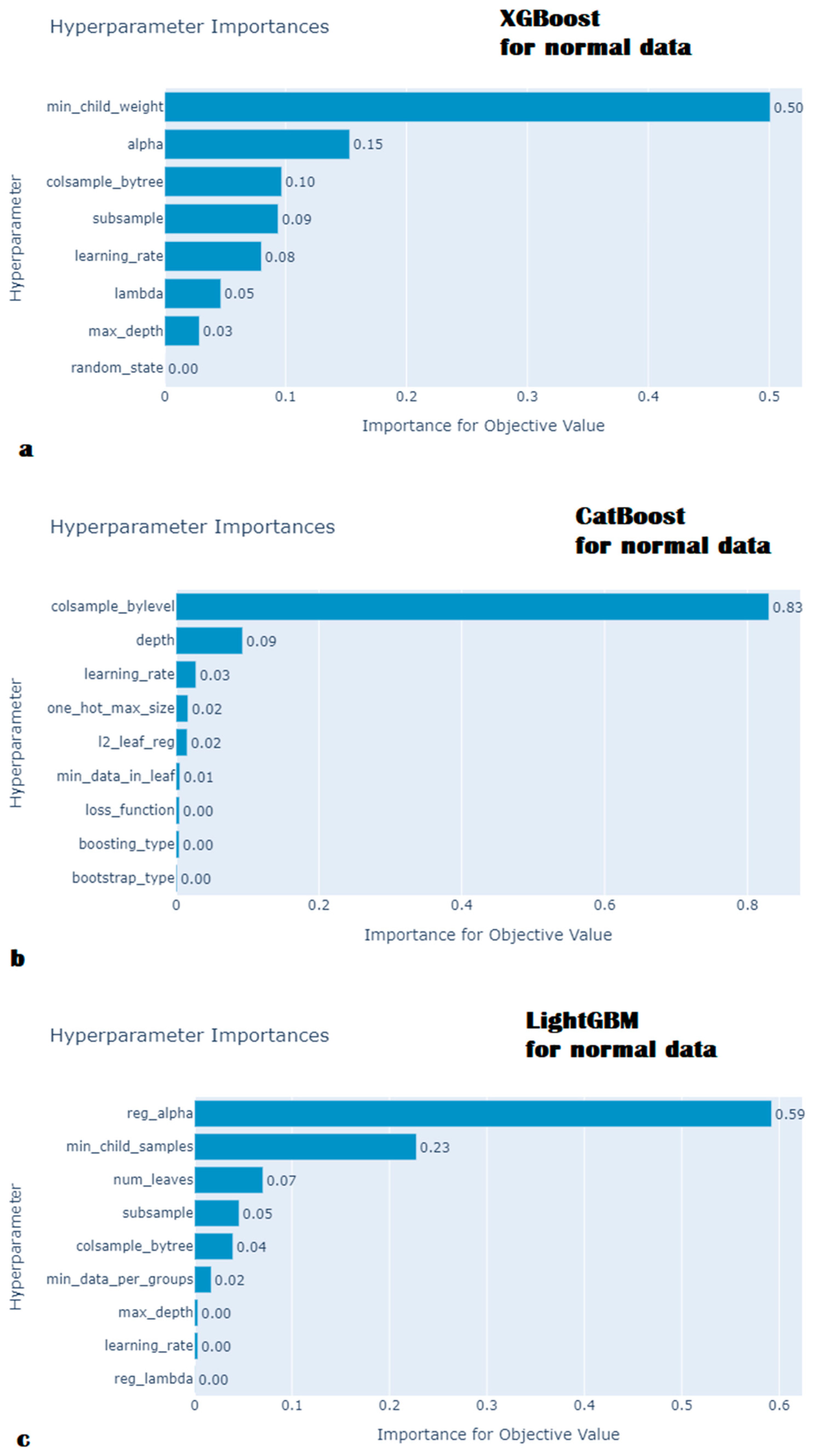
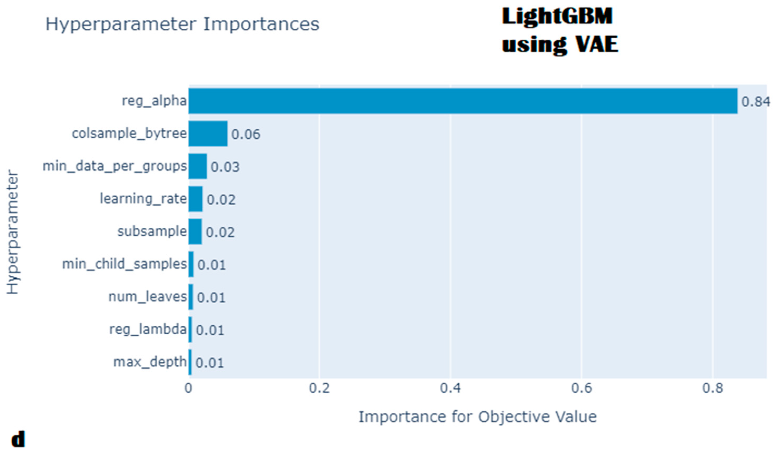
Hyperparameter optimization
The efficiency of Catboost, XGBoost and LightGBM depends a lot on the optimal selection of the hyperparameters, because they use the gradient boosting framework, i.e., boosting ensemble learning, and are prone to overfitting if they are not properly parameterized [19]. Thus, Optuna (a hyperparameter optimization technique) was used for hyperparameter tuning of the three models [42]. Optuna allows a large combination of hyperparameters to be tested quickly and efficiently. A total of 400 trials with different combinations of hyperparameters for each model were tested and the combination of parameters that minimized the MAE were selected. The optimized hyperparameters for all models are presented in Table 1. The min_child_weight, colsample_bylevel, reg_alpha parameters were identified as the most influential for the XGBoost, CatBoost, and LightGBM models, respectively.
d.
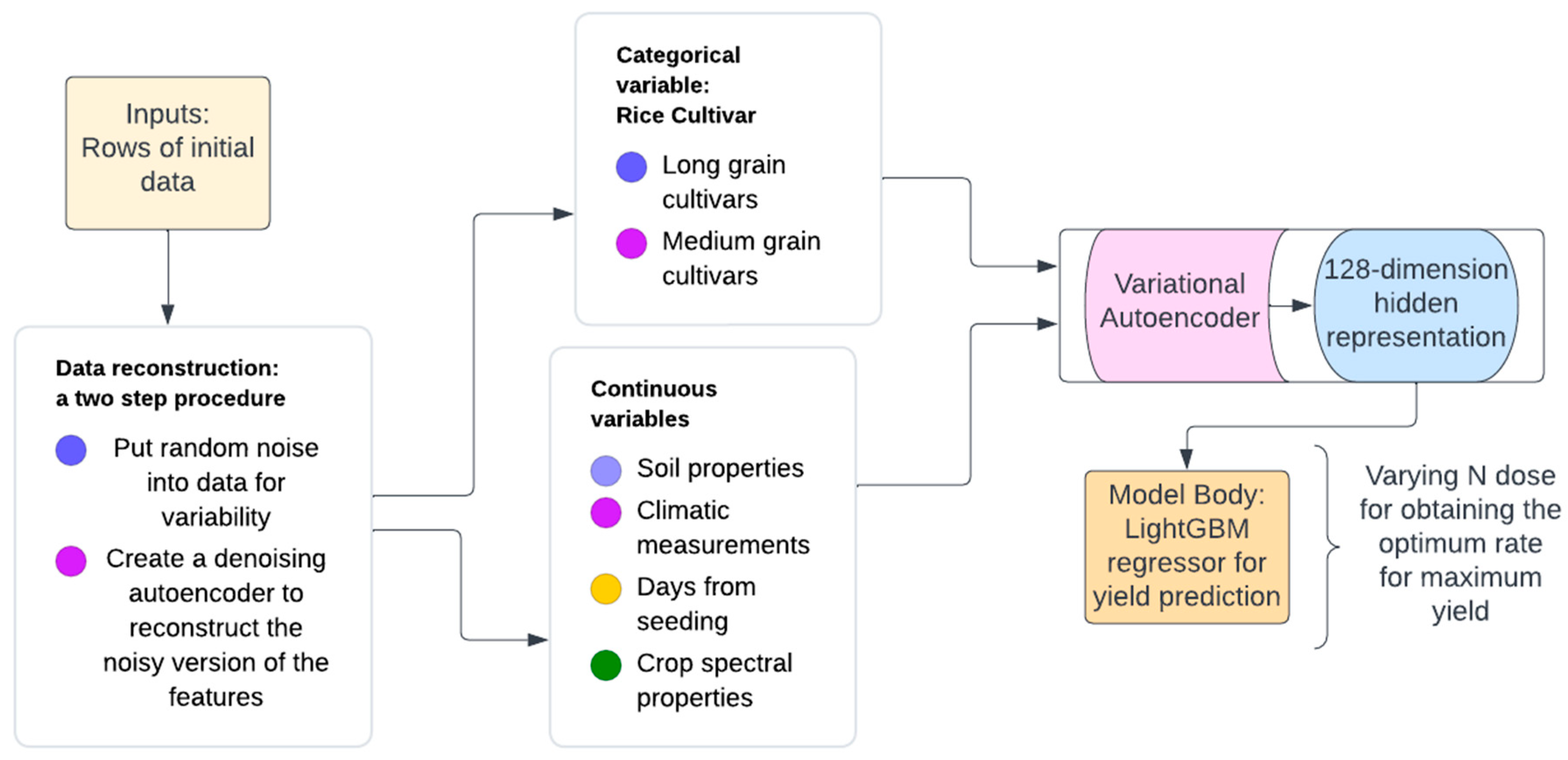
Variational autoencoder
To avoid affection of the ML algorithms by any discrepancy or noise in the initial dataset, an innovative technique was used, namely the variational autoencoder (VAE). Discrepancy and noise are inherent in data coming from environmental and agricultural resources due to high within- and between-field variance, which can affect the output of an ML yield prediction algorithm.
VAE reduces the effect of an observation that does not conform to normal patterns in the data [43], by performing reconstruction of the input data before feeding them into the ML algorithms, so that the obtained output is given to the ML algorithm as input for training the model. Reconstruction is based on the intrinsic properties of the input data and does not require the target data, i.e., yield for the present work. Thus, VAE learns the original input data representation and transforms them in a latent feature space. The latent feature space obtained by the VAE is clean and represents normal behavior compared to the initial data providing though a more abstract representation of the original data.
The Fast.ai framework was used for constructing the VAE for the scopes of the present study [37]. The mean R2 for all continuous variables between the predicted transformed variables and the initial normal data was equal to 0.90. The accuracy for the categorical variable, i.e., variety, was 0.94. As the correlation between the transformed representation and the initial normal data was quite strong, the compressed data could be used to build a better model.
A neural network for the autoencoder was settled on 1024 nodes and finally a 128-dimension hidden representation was obtained for the encoder. The latent features were given to the three ML algorithms, and the hyperparameter tuning procedure using Optuna was followed again, providing new hyperparameters that are presented in Table 2. The importance of the hyperparameters is shown in Figure 2.
e.
SHAP analysis
To shed light on the underlying factors that influence rice yield according to the fitted ML models, Shapley additive explanations (SHAP) analysis was used [44,45]. SHAP is an XAI (explainable artificial intelligence) technique adopting a concept coming from game theory and reflects a feature’s influence on a model’s prediction [46,47]. SHAP generates a value (a Shapley value) by changing the input data for all rows and for all features, keeping all the data equal to the initial and varying one for each trial.
Thus, SHAP values are calculated for each prediction separately and explain a single prediction. They finally calculate the difference between the model’s prediction and the prediction generated by varying a feature in the row. If the sum of differences is highly positive, then the feature is highly important and has a positive correlation with the prediction for this specific row. If the sum of differences is highly negative, the feature has a negative correlation with the prediction and if the sum of differences is close to zero, the feature has low importance.
In practice, SHAP builds a small explainer model for a single observation to explain how the prediction was achieved by the model for this observation. Finally, the benefit from this procedure is that for each specific row the contribution of each feature can be assessed regardless of the underlying model [48]. This is highly important for nonlinear methods, such as CatBoost, LightGBM, XGBoost, because—even though these algorithms are powerful and reduce error in the predictions—it is difficult to understand how the output was obtained.
Matplotlib and seaborn were used to make visualizations [49,50]. The SHAP library was used for constructing the visualizations of feature importance and SHAP dependence plots. Data analysis, model construction and visualizations were carried out using Python [51].

3. Results

  • Model performance
The mean absolute error (MAE) for the CatBoost model was lower than the LightGBM and XGBoost yield models for the hindcast data. MAE for CatBoost, XGBoost and LightGBM rice yield models were equal to 0.576, 0.581 and 0.583 tn/ha, respectively. The CatBoost model for the forecasting climatic data gave a slightly higher MAE of 0.6 tn/ha.
The feature important plot for the CatBoost model based on the hindcast data is presented in Figure 3a. The calculated rolling mean of SAR backscatter values for four consecutive images in June (SAR_VH_June_rolling_mean) was identified as the most influential parameter for the yield model. For more detailed information on the SAR backscatter values for crop monitoring, see [52]. The variety variable (long or medium grain) was the second most influential parameter for the yield model. The LNC parameter divided by the days from seeding (LNC/Days_from_seeding) was the third most influential parameter.
The SAR_VH_June/Days_from_seeding, the values obtained by the last SAR image in June divided by the days from seeding, was identified as the fourth most significant feature. The LNC and the backscatter values obtained by SAR imagery were divided by the days from seeding, because the LNC and SAR values increase as plant growth increases and thus normalization is necessary for capturing the maximum information from these indices. The N need for rice crop was identified as the sixth most important feature according to the CatBoost model. Silt, which is a kind of mineral particle related to soil density, was identified as the most significant soil attribute.
The feature importance plot for the yield model based on the forecast climate data is presented in Figure 3b. Only the mean precipitation of May was based on hindcast data because May precipitation was available at the time of preparing the recommendation advice (end of June). The N need variable dropped from 6th to 10th position in the order of feature importance.
Fitting the CatBoost, LightGBM and XGBoost models with the reconstructed data using VAE and including only the forecasts for the climate data, the LightGBM model gave the lowest MAE, i.e., MAE for LightGBM, XGBoost and CatBoost rice yield models using VAE were equal to 0.576, 0.583 and 0.6 tn/ha, respectively. Thus, MAE for LightGBM using VAE was lower compared to the CatBoost model fitted on the normal data including the forecasting climate data (0.6 tn/ha) and equal to the MAE obtained by the CatBoost model fitted on the normal data including the hindcast climate data.
b.
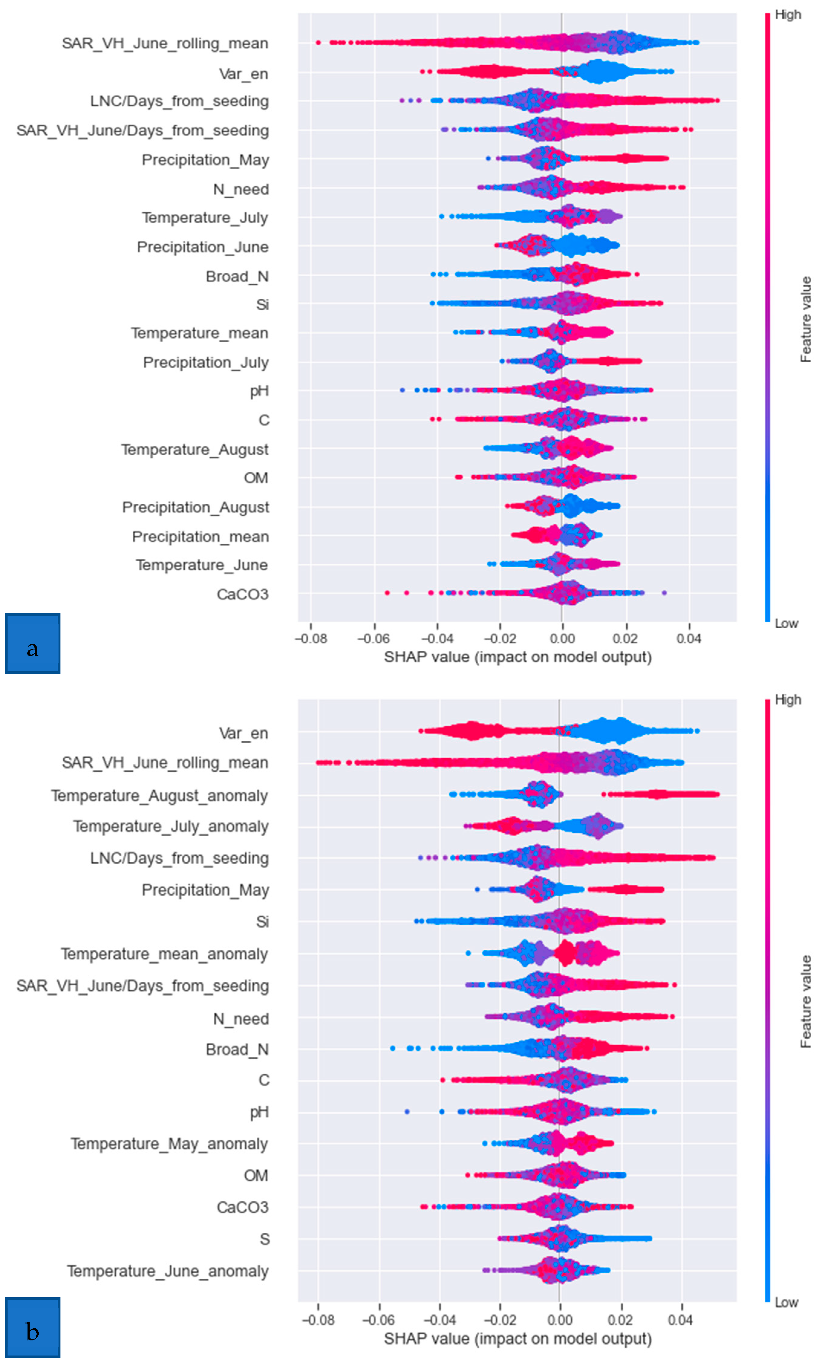
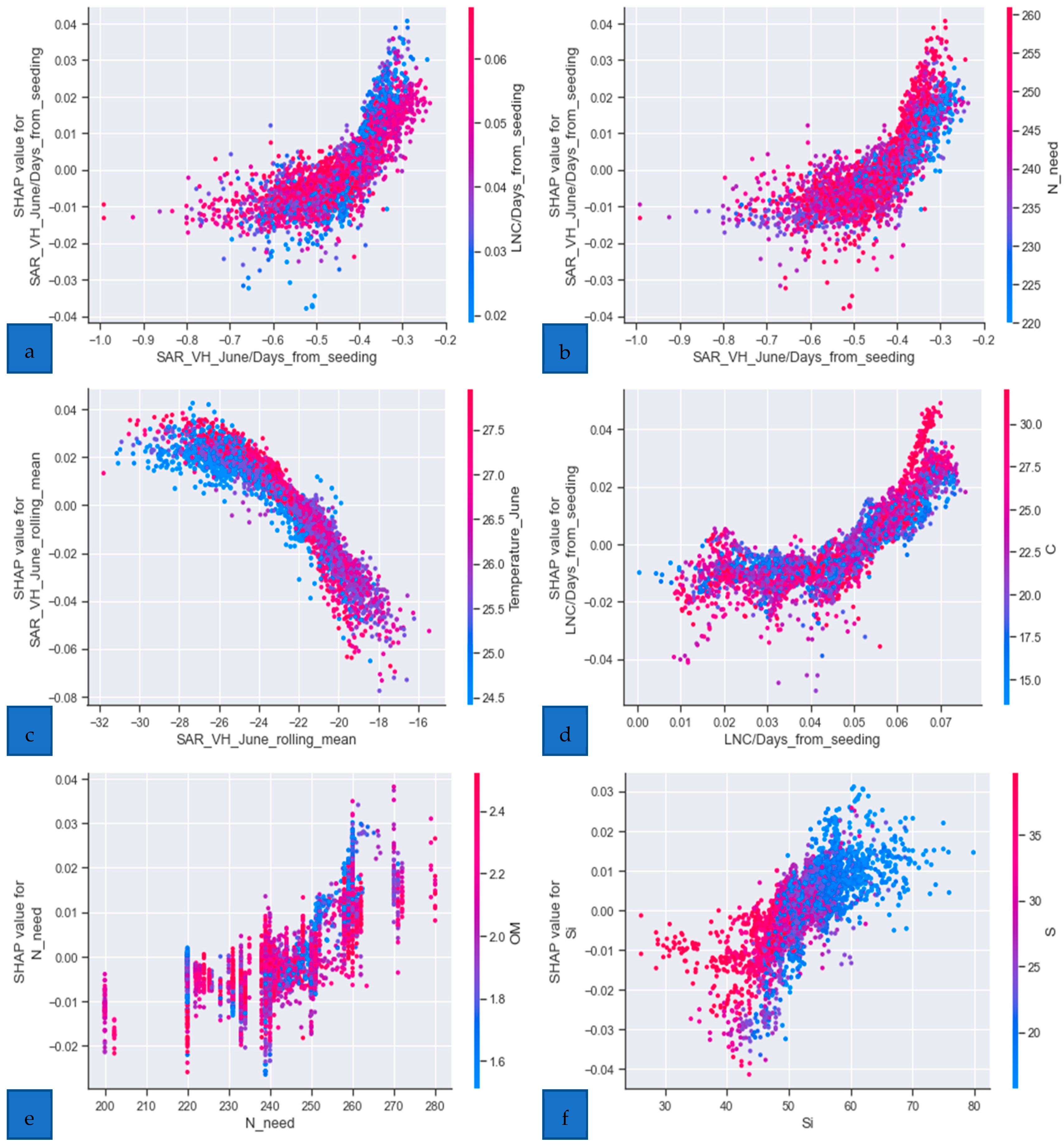
Model explanation with SHAP
SHAP dependence plots show that yield increases as the SAR backscatter by image taken just before N topdressing and divided by the days from seeding increases and present the interactions that exist between SAR backscatter with LNC and N (Figure 4a,b). Thus, for high SAR values, if the LNC is high, the N need is low and vice versa. There was a negative correlation between the mean SAR backscatter by all the June images and the predicted yield and a positive correlation between LNC divided by the days from seeding and predicted yield (Figure 4c,d).
N need showed a positive correlation with the predicted yield having its strongest correlation with the organic matter content of soil (Figure 4e). Thus, the yield is high for high N rate when the organic matter in soil is low. Silt had a positive correlation with the predicted yield and its strongest interaction was with the sand content of soil (Figure 4f). As the silt content in soil increases, the predicted yield increases and the sand content in the soil is reduced.
c.
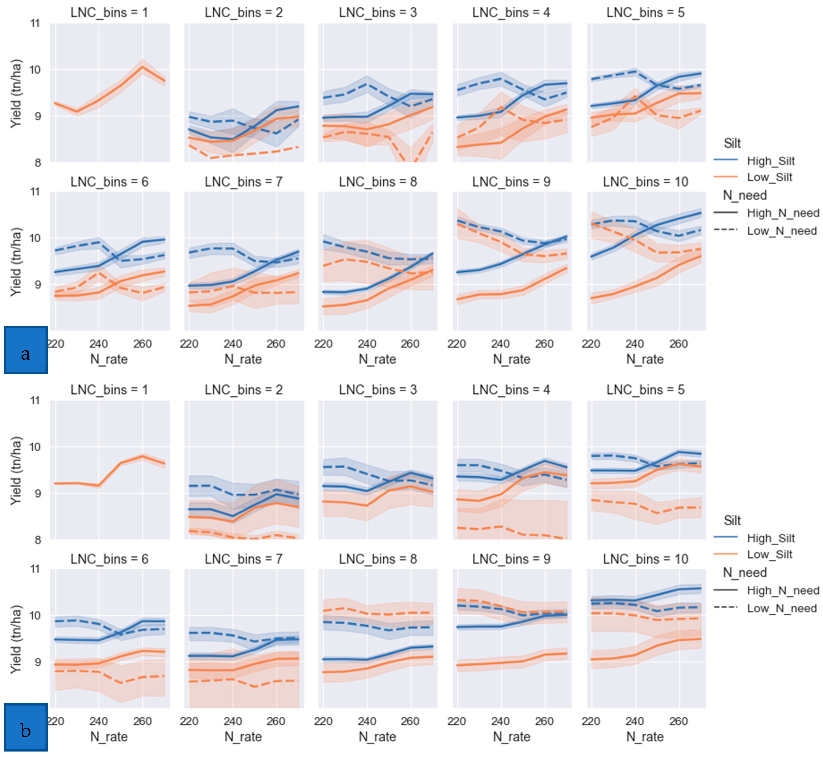
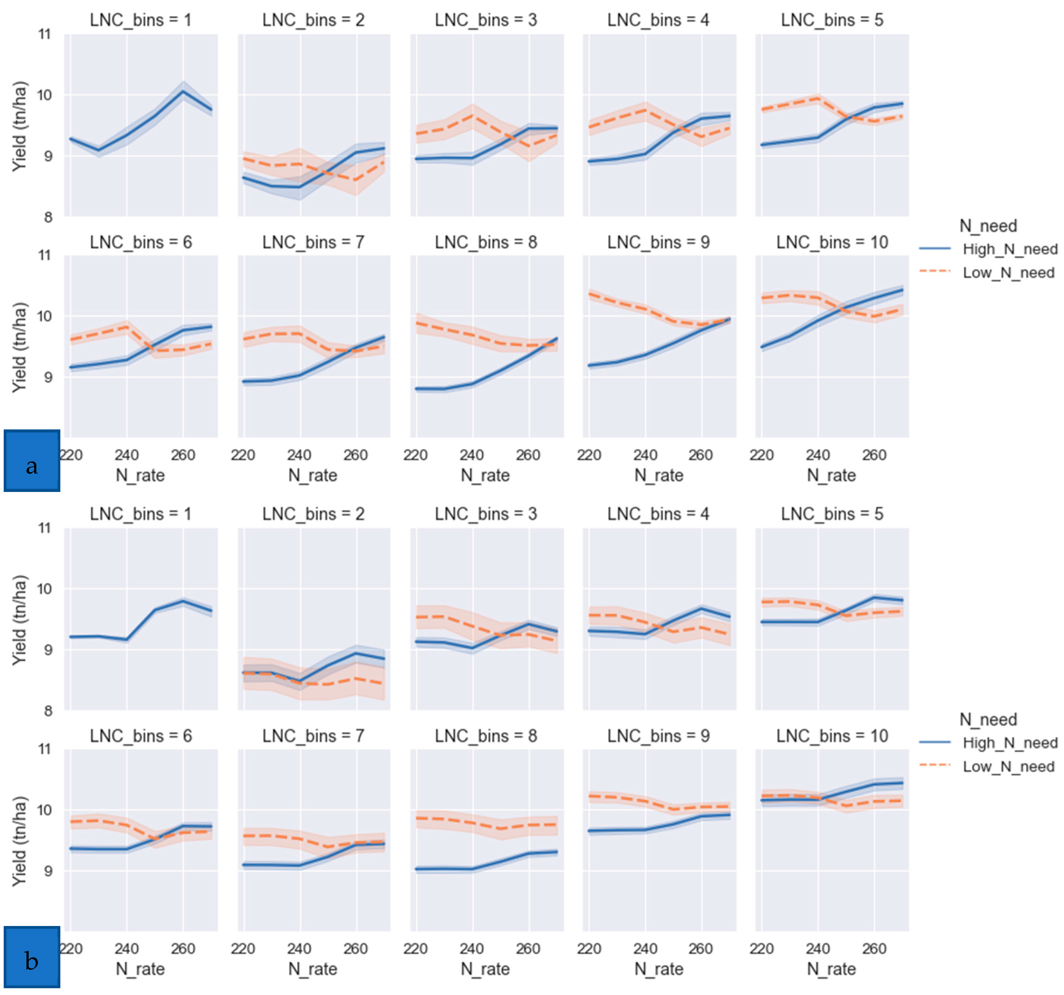
Yield response curves to N fertilization
Yield curves were created according to different N levels for evaluating the effect of N rate on the yield prediction according to the CatBoost model for the normal data and the LightGBM model for reconstructed data using VAE. The LNC was separated into different equally sized discrete bins according to the LNC levels. Then, curves of yield prediction according to the trained algorithm were fitted for various N levels to select the N dose maximizing yield for each LNC bin. According to the yield curves, the optimum N fertilization dose is determined where yield begins to decrease [2,53,54]. The LNC bins were discretized as follows: (1) 0.19–0.34, (2) 0.34–0.62, (3) 0.62-0.92, (4) 0.92–1.22, (5) 1.22–1.52, (6) 1.52–1.82, (7) 1.82–2.12, (8) 2.12–2.42, (9) 2.42–2.72 and (10) 2.72–3.02.
Silt was also discretized in two bins for soils with low silt levels, i.e., from 26.6 to 46.14% and for high silt levels, i.e., 46.14 to 66.13%, as silt was identified as a significant soil parameter by the CatBoost model. Figure 5 shows the yield curves provided by the CatBoost and LightGBM models, across various N levels, for reconstructed data using VAE and normal data for the various LNC bins, respectively. The dashed lines show soil units (grids) where yield is maximized for N rate less than 250 kg/ha. The yield curves on the reconstructed data by the VAE in Figure 5a show that for soils where yield is maximized for N rate less than 250 kg/ha, yield increases up to 240 kg/ha for the LNC bins 2 to 7 and then starts reducing. Yield is maximized at 220 kg/ha for soils with low N requirement only for high LNC values, i.e., for LNC bins from 8 to 10. On the other hand, yield curves on normal data show that yield is always maximum at the lower rate, i.e., 220 kg/ha, for soils with low N requirement across all LNC bins.
Figure 6a shows that for low silt levels and high LNC values, i.e., for LNC bins from 8 to 10, rice yield was reduced at greater rate as N rate increased compared to rice plants grown in soils with high silt levels according to the LightGBM model using VAE. On the contrary, Figure 6b shows that for normal data, LNC bins from 8 to 10, and low N need rice plants, there was no effect of N rate on rice yield.
Leaf nitrogen content (LNC) obtained by Sentinel-2 imagery at the end of June, i.e., some days before nitrogen topdressing, was higher for 2017 than all other years (Figure 7a). This correlated with higher mean precipitation in May compared to other years (Figure 7b). The coolest June was in 2020, and this correlated with lower LNC for 2020 compared to all other years (Figure 7c). Significantly lower yield was obtained for the medium grain rice variety (cv. Ronaldo) in 2020 compared to the other years (p < 0.001). On the other hand, significantly higher yield was harvested in 2017 for both medium- and long-grain varieties compared to all other years (p < 0.001) (Figure 3b).

4. Discussion

  • N need as a significant determinant of the model
The N application rate (N_need) is the sixth most important parameter, which was expected, as N is required by the rice crop in the largest quantity and is the most limiting factor in rice productivity if not supplied by fertilizers. Thus, N was identified as a significant predictor for the model, which is an improvement of the current algorithm compared to the model published by Iatrou et al. [2].
The MAE presented for the current rice yield model (0.576 tn/ha with the hindcast climate data and 0.576 with the forecast data using VAE) is lower compared to the 0.629 tn/ha MAE and 0.73 tn/ha root mean square (RMS) presented by Iatrou et al. [2]. However, this difference in the error was expected, as more data were gathered for 5 consecutive years, providing a better algorithm for rice yield prediction and the current work included more information, such the SAR backscatter and climate data.
b.
The importance of SAR backscatter on the model’s performance
Feature evaluation showed that the SAR backscatter rolling mean is the most significant parameter for the CatBoost yield model trained on the hindcast climate data. As expected, the variety (Var_en) was the second most important parameter, because the long grain rice varieties are less productive compared to the medium-grain rice varieties. Interestingly, the mean precipitation of May and the mean temperature of July were the fifth and seventh most important parameters for rice yield. It is generally known that the weather interacts with N on crop yield, because environmental factors, such as temperature and rain, exert a large influence on seasonal N mineralization and availability in soil [55,56].
c.
Water effect on rice productivity
High precipitation in July and May correlates with high yield, unlike June precipitation, which correlates with low yield, as shown in Figure 7a. High precipitation in May and July ensures water sufficiency for the rice crop because water is limiting for rice growing in Greece, especially for intense summer droughts. If the growers fail to establish a flood on rice fields and there are periods of water draining, there is an aerobic period in soil, resulting in nitrification. When the field is reflooded and becomes anaerobic, the N is lost as N2O [1,57]. On contrary, if the weather is rainy in June, growers tend to drain their rice fields for longer, because June is the time of herbicide application. Thus, despite the water being sufficient for establishing a permanent flood, the growers tend to drain their fields for longer, aiming at finding a time window without rain for targeting the weeds, and inevitably the N losses are high.
The effect of precipitation in May and July on yield is due to the uptake of N, as establishing a permanent flood for longer results in reduced N losses. According to Espino et al. [24], rice plants growing in deep water are taller throughout the season and this is probably linked with LNC index. Thus, the LNC probably depicts both the N uptake and the size of the rice plants. Using SHAP dependence analysis, though, which displays the effect of LNC on yield (Figure 4d), the yield was shown to increase with increased LNC according to the yield prediction model. This could probably be because of the increased N uptake during the early stages of plant growth (May–June) and not because of the size of the plant, as Espino et al. [24] found that tall plants are not necessarily more productive than short plants.
However, as yield and LNC in June of 2017 crop season were significantly higher than the other crop seasons, these data also confirm previous studies on rice claiming that N losses at the beginning of the cropping season result in yield losses that later cannot be restored by increased topdressing N fertilization [1]. This is shown in Figure 5a,b, where the maximum yield is obtained for high LNC values, i.e., LNC bin from 9 and 10. For very low LNC values, i.e., LNC bin equal to 1, yield increases with N rate increase, but cannot outreach 10 tn/ha.
A frequently used operational farming practice currently in Greece includes a low N rate before seeding, keeping waters very low for long periods for controlling the weeds efficiently with herbicides, and applying a high dose of N at topdressing reaching in total 260 to 270 kg/ha, as growers know from experience that this is a safe way of obtaining high yields (close to 10 tn/ha). The results of the current study confirm this operational perception, as rice plants belonging to LNC bin 1 can reach high yields with excessive N fertilization, as shown in Figure 5a. However, with the current levels of fertilizer prices, —925, 315, 170 US dollars per metric ton for June 2022, May 2021, and May 2017—following a conservative cultural practice with reduced N losses and low N rates is crucial for rice growers nowadays.
Furthermore, having the plants starving for N does not ensure that the plants will uptake low N, as there are plants grown on fertile soils having high organic matter levels, high clay content and high-water availability and thus these plants will not necessarily have low LNC levels. Applying the currently developed ML model using VAE in practice can aid the growers obtain high yields with lower N rates. This proves that the capacity of the currently developed prediction model using VAE has high commercial benefit for rice growing, as the model can identify areas within the crop with high or low N requirement and recommend high or low N fertilization at topdressing, respectively.
d.
The effect of soil texture on rice productivity
Twelve percent of the experimental area consists of clay soils, while 87% of the fields are silty, loamy, or sandy loamy. This is probably why silt was identified as the most important soil attribute by feature evaluation using SHAP for the yield model. According to the growers’ experience, rice crops grown on sandy soils or soils with low content in clay or silt tend to be more vulnerable to high N doses. This was clearly identified by the ML model using VAE, as shown in Figure 6a, because for the high LNC values, i.e., LNC bins from 8 to 9, and for the rice crops with low N requirement, yield drop was greater, with N rate increase for the soils with low silt content. There are many references in the literature showing that excessive N fertilization in sandy soils affects root anchorage, rice lodging, and finally yield [58,59,60]. According to commercial experience, rice crops in sandy soils obtaining high growth can sometimes be disappointingly low in yield.
e.
The importance of VAE for accurately predicting the N requirements
The results of the current study show that reconstructed data using VAE gave a significant improvement on the yield prediction algorithm compared to the normal data. The relationships between N and predicted yield better described the real conditions in field, as is known from commercial experience, and the yield model using VAE and based on forecasting climate data gave an equal MAE to the yield model using normal data and hindcast climate data.
Furthermore, the model trained on the normal data showed that for the low-N-requirement rice plants, the yield was always maximum at the lowest rate (220 kg N/ha) across the different LNC values, which does not agree with the commercial experience, as rice crops under the Greek rice growing conditions rarely provide high yields when supplied with 220 kg/ha N (Figure 5b). The improvement in the yield prediction model using VAE relies mainly on the optimization of the variance inherent in the environmental and weather data. The improved performance of the model using the reconstructed data by the VAE was rewarded in the operational application of the model, as there was an increase for the yield of 2022 cropping season of 4.32% compared to the average of 2017–2021 cropping seasons.
An overview of the role of the VAE in data treatment and processes is presented in Figure 8.
f.
SHAP analysis shedding light on the model
SHAP analysis clarified the effect of variables on yield prediction and their interactions. Interestingly, there was a significant interaction between SAR backscatter with LNC and N need (Figure 4a,b). If the LNC was low, the N need was high for high SAR values and vice versa. This shows that the model can identify rice plants having high N need due to reduced N uptake (low LNC). An interesting finding was, also, the negative correlation of the SAR rolling mean (all June SAR images) with yield, because probably the early SAR images can identify water within the rice lagoons, which is critical for rice growing and N uptake. SAR rolling mean interacts significantly with temperature, as June temperature correlates with plant growth and N uptake affecting rice yield. In addition, there is positive correlation between LNC, N need and silt with the predicted yield.
Unsurprisingly, the most significant interaction for N need is the organic matter content of soil. Thus, for high N doses the yield increases for the low fertility soils with low organic matter, as there is increased release of available N from soil organic matter [61]. Soil density also plays a significant role in rice growing, as mentioned above, and thus silt has a positive relation with the predicted yield (Figure 4f).

5. Conclusions

This research was focused explicitly on empirical modeling, an option justified by the operational direction of the attempt and rewarded by the results. Data reconstructed by a VAE provided a more sophisticated and detailed ML model, improving our knowledge about the various correlations between the soil, N management parameters and yield. Moreover, the development of the ML project allowed us to discover patterns, such as the improved yield potential by reducing N rate when the rice crop has properly grown from seeding to topdressing with reduced N losses.
Apart from the current approach itself, the fact that both types of the satellite data used (optical and radar) were found at the highest levels of importance for the employed ML algorithms, together with their combination as input variables in the rice yield prediction modeling, could be seen as innovative points of this research. Use of a high-resolution grid (30 × 30 m), which facilitates holistic multisource data treatment, could also be seen as a novelty of the approach. Such a grid facilitates easy and fast conversion of output data into detailed site-specific fertilization maps for automated applications with variable-rate technologies (VRT).
Yield prediction can never be perfect, as yield can be affected by the weather even at the late stages of plant growth. However, the scope of the yield prediction model presented here is to estimate the N dose that will potentially maximize yield. Even modest benefit from the yield prediction model can make a big difference, as a small yield increase or N savings may affect the economics of the agricultural enterprise. Indicatively, the average yield in 2022 rice cultivation in the study fields (with N-recommendations based on the current analysis) increased by 4.32% compared to the previous 5 years of experimentation in the same fields (9.96 t/ha vs. 9.54 t/ha). We should not also ignore environmental protection (because of the reported fertilizer input reduction) and cropping land sustainability (because of the potential soil fertility maintenance).

Author Contributions

Conceptualization, C.K., S.M. and M.I.; Methodology, M.I. and C.K.; Software, X.T. and M.I.; Formal analysis, M.I. and X.T.; Investigation, X.T. and S.M.; Data curation, X.T. and C.K.; Visualization: X.T. and C.K.; Writing—original draft, M.I., X.T. and C.K.; Writing—review & editing, C.K. and M.I.; Supervision, S.M. Project administration, S.M. All authors have read and agreed to the published version of the manuscript.

Funding

This research received no external funding.

Data Availability Statement

Not applicable.

Acknowledgments

Cordial thanks to Kostas Kravvas for contributing with his rice farm and agricultural machinery and for his dedicated support to this study.

Conflicts of Interest

The authors declare no conflict of interest.

References

  1. Williams, J.F. Rice Nutrient Management in California; University of California: Oakland, CA, USA, 2010. [Google Scholar]
  2. Iatrou, M.; Karydas, C.; Iatrou, G.; Pitsiorlas, I.; Aschonitis, V.; Raptis, I.; Mpetas, S.; Kravvas, K.; Mourelatos, S. Topdressing nitrogen demand prediction in rice crop using machine learning systems. Agriculture 2021, 11, 312. [Google Scholar] [CrossRef]
  3. Iatrou, M.; Karydas, C.; Iatrou, G.; Zartaloudis, Z.; Kravvas, K.; Mourelatos, S. Optimization of fertilization recommendation in Greek rice fields using precision agriculture. Agric. Econ. Rev. 2018, 19, 64–75. [Google Scholar]
  4. Borgnis, F.; Pedroli, E. Technological Interventions for Obsessive–Compulsive Disorder Management. Compr. Clin. Psychol. 2022, 10, 283–306. [Google Scholar]
  5. Viana, C.M.; Santos, M.; Freire, D.; Abrantes, P.; Rocha, J. Evaluation of the factors explaining the use of agricultural land: A machine learning and model-agnostic approach. Ecol. Indic. 2021, 131, 108200. [Google Scholar] [CrossRef]
  6. Chen, T.; Guestrin, C. XGBoost: A Scalable Tree Boosting System. In Proceedings of the 22Nd ACM SIGKDD International Conference on Knowledge Discovery and Data Mining, New York, NY, USA, 13 August 2016; ACM: New York, NY, USA, 2016; pp. 785–794. [Google Scholar]
  7. Horie, T.; Nakagawa, H.; Centeno, G.; Kropff, M. The Rice Simulation Model SIMRIW and Its Testing. In Modeling the Impact of Climate Change on Rice Production in Asia CABI, UK, IRRI, Philippines; Matthews, R.B., Kropff, M.J., Bachelet, D., van Laar, H.H., Eds.; CAR international: Manila, Philippines, 1999; pp. 95–139. [Google Scholar]
  8. Tang, L.; Zhu, Y.; Hannaway, D.; Meng, Y.; Liu, L.; Chen, L.; Cao, W. RiceGrow: A rice growth and productivity model. NJAS Wagening. J. Life Sci. 2009, 57, 83–92. [Google Scholar] [CrossRef] [Green Version]
  9. Bouman, B.; Kropff, M.; Tuong, T.P.; Wopereis, S.; ten Berge, H.; van Laar, H. ORYZA2000: Modeling Lowland Rice; IRRI: Los Baños, Philippines, 2001. [Google Scholar]
  10. Mahmood, R.; Meo, M.; Legates, D.R.; Morrissey, M.L. The CERES-Rice Model-Based Estimates of Potential Monsoon Season Rainfed Rice Productivity in Bangladesh. Prof. Geogr. 2003, 55, 259–273. [Google Scholar]
  11. Gómez, D.; Salvador, P.; Sanz, J.; Casanova, J.L. Potato yield prediction using machine learning techniques and Sentinel 2 data. Remote Sens 2019, 11, 1745. [Google Scholar] [CrossRef] [Green Version]
  12. Boote, K.; Jones, J.; Pickering, N. Potential Uses and Limitations of Crop Models. Agron J. 1996, 88, 704–716. [Google Scholar] [CrossRef]
  13. Jeong, S.; Ko, J.; Yeom, J.-M. Predicting rice yield at pixel scale through synthetic use of crop and deep learning models with satellite data in South and North Korea. Sci. Total Environ. 2021, 802, 149726. [Google Scholar] [CrossRef] [PubMed]
  14. Liu, K.; Deng, J.; Lu, J.; Wang, X.; Lu, B.; Tian, X.; Zhang, Y. High Nitrogen Levels Alleviate Yield Loss of Super Hybrid Rice Caused by High Temperatures During the Flowering Stage. Front. Plant Sci. 2019, 10, 357. [Google Scholar] [CrossRef] [PubMed] [Green Version]
  15. Maina, S.C.; Bryant, R.E.; Ogallo, W.O.; Varshney, K.R.; Speakman, S.; Cintas, C.; Walcott-Bryant, A.; Samoilescu, R.-F.; Weldemariam, K. Preservation of Anomalous Subgroups On Variational Autoencoder Transformed Data. In Proceedings of the ICASSP 2020—2020 IEEE International Conference on Acoustics, Speech and Signal Processing (ICASSP), Barcelona, Spain, 4–8 May 2020; IEEE: Piscataway, NJ, USA; pp. 3627–3631. [Google Scholar]
  16. Karydas, C.G.; Silleos, N.G. Precision Agriculture: Method Description—Current Status and Perspectives. In Special Conference on “Informatics in Agricultural Sector”, 2nd ed.; Matsatsinis, N., Ed.; New Technologies Publications: Chania, Greece, 2000; pp. 134–146. [Google Scholar]
  17. International Society of Precision Agriculture. 2022. Available online: https://www.ispag.org/ (accessed on 5 October 2022).
  18. Litskas, V.D.; Aschonitis, V.G.; Lekakis, E.H.; Antonopoulos, V.Z. Effects of land use and irrigation practices on Ca, Mg, K, Na loads in rice-based agricultural systems. Agric. Water Manag. 2014, 132, 30–36. [Google Scholar] [CrossRef]
  19. Karydas, C.; Iatrou, M.; Iatrou, G.; Mourelatos, S. Management zone delineation for site-specific fertilization in rice crop using multi-temporal rapideye imagery. Remote Sens. 2020, 12, 2604. [Google Scholar] [CrossRef]
  20. Iatrou, M.; Papadopoulos, A.; Dichala, O.; Psoma, P.; Bountla, A. Determination of Soil Available Phosphorus using the Olsen and Mehlich 3 Methods for Greek Soils Having Variable Amounts of Calcium Carbonate. Commun. Soil Sci. Plant Anal. 2014, 45, 2207–2214. [Google Scholar] [CrossRef]
  21. Du, G.; Liu, W.; Pan, T.; Yang, H.; Wang, Q. Cooling Effect of Paddy on Land Surface Temperature in Cold China Based on MODIS Data: A Case Study in Northern Sanjiang Plain. Sustainability 2019, 11, 5672. [Google Scholar] [CrossRef] [Green Version]
  22. Hussain, S.; Khaliq, A.; Ali, B.; Hussain, H.A.; Qadir, T.; Hussain, S. Temperature Extremes: Impact on Rice Growth and Development. In Plant Abiotic Stress Tolerance: Agronomic, Molecular and Biotechnological Approaches; Springer International Publishing: Cham, Switzerland, 2019; pp. 153–171. [Google Scholar]
  23. Skofronick-Jackson, G.; Petersen, W.A.; Berg, W.; Kidd, C.; Stocker, E.F.; Kirschbaum, D.B.; Kakar, R.; Braun, S.A.; Huffman, G.J.; Iguchi, T.; et al. The Global Precipitation Measurement (GPM) Mission for Science and Society. Bull. Am. Meteorol. Soc. 2017, 98, 1679–1695. [Google Scholar] [CrossRef]
  24. Espino, L.; Leinfelder-Miles, M.; Brim-Deforest, W.; Al-khatib, K.; Linquist, B.; Swett, C. Rice Production Manual. In Agriculture and Natural Resources; University of California: Berkeley, CA, USA, 2018. [Google Scholar]
  25. Domsch, H.; Heisig, M.; Witzke, K. Estimation of yield zones using aerial images and yield data from a few tracks of a combine harvester. Precis. Agric. 2008, 9, 321–337. [Google Scholar] [CrossRef]
  26. Gemtos, T.; Fountas, S.; Blackmore, B.S.; Greipentrog, H.W. Precision Farming Experience in Europe and the Greek Potential. In Proceedings of the 1st Hellenic Conference in Information Technology in Agriculture (HAICTA), Athens, Greece, 6–7 June 2002. [Google Scholar]
  27. Evans, J.R. International Association for Ecology Photosynthesis and Nitrogen Relationships in Leaves of C3 Plants. Oecologia 1989, 78, 9–19. [Google Scholar] [CrossRef]
  28. Ladha, J.K.; Pathak, H.; Krupnik, T.J.; Six, J.; van Kessel, C. Efficiency of Fertilizer Nitrogen in Cereal Production: Retrospects and Prospects. Adv. Agron. 2005, 87, 85–156. [Google Scholar]
  29. Stroppiana, D.; Fava, F.; Boschetti, M.; Brivio, P.A. Estimation of Nitrogen Content in Crops and Pastures Using Hyperspectral Vegetation Indices. In Hyperspectral Remote Sensing of Vegetation; Thenkabail, P.S., Lyon, J.G., Huete, A., Eds.; CRC Press: Boca Raton, FL, USA, 2011; pp. 245–262. [Google Scholar]
  30. Karydas, C. Temporal dimensions in rice crop spectral profiles. J. Geomat. 2016, 10, 140–148. [Google Scholar]
  31. Westfall KLF & DGDWWMCB. Evaluating Farmer Defined Management Zone Maps for Variable Rate Fertilizer Application. Precis. Agric. 2000, 2, 201–215. [Google Scholar] [CrossRef]
  32. Heijting, S.; de Bruin, S.; Bregt, A.K. The arable farmer as the assessor of within-field soil variation. Precis. Agric. 2011, 12, 488–507. [Google Scholar] [CrossRef] [Green Version]
  33. Kumar, L.; Mutanga, O. Google Earth Engine applications since inception: Usage, trends, and potential. Remote Sens. 2018, 10, 1509. [Google Scholar] [CrossRef] [Green Version]
  34. Gorelick, N.; Hancher, M.; Dixon, M.; Ilyushchenko, S.; Thau, D.; Moore, R. Google Earth Engine: Planetary-scale geospatial analysis for everyone. Remote Sens. Environ. 2017, 202, 18–27. [Google Scholar] [CrossRef]
  35. Amani, M.; Ghorbanian, A.; Ahmadi, S.A.; Kakooei, M.; Moghimi, A.; Mirmazloumi, S.M.; Moghaddam, S.H.A.; Mahdavi, S.; Ghahremanloo, M.; Parsian, S.; et al. Google Earth Engine Cloud Computing Platform for Remote Sensing Big Data Applications: A Comprehensive Review. IEEE J. Sel. Top. Appl. Earth Obs. Remote Sens. 2020, 13, 5326–5350. [Google Scholar] [CrossRef]
  36. Breiman, L. Random forests. Mach. Learn. 2001, 45, 5–32. [Google Scholar] [CrossRef]
  37. Howard, J.; Gugger, S. Deep Learning for Coders with Fastai and PyTorch; O’Reilly Media: Sebastopol, CA, USA, 2020. [Google Scholar]
  38. Dorogush, A.V.; Gulin, A.; Gusev, G.; Kazeev, N.; Prokhorenkova, L.O.; Vorobev, A. Fighting Biases with Dynamic Boosting; CoRR: 2017; abs/1706.0. Available online: http://arxiv.org/abs/1706.09516 (accessed on 16 May 2022).
  39. Ke, G.; Meng, Q.; Finley, T.; Wang, T.; Chen, W.; Ma, W.; Ye, Q.; Liu, T.-Y. LightGBM: A Highly Efficient Gradient Boosting Decision Tree. In Advances in Neural Information Processing Systems; Guyon, I., von Luxburg, U., Bengio, S., Wallach, H., Fergus, R., Vishwanathan, S., Eds.; Curran Associates, Inc.: Nice, France, 2017. [Google Scholar]
  40. Abdullahi, I.A.; Raheem, L.; Muhammed, M.; Rabiat, O.; Ganiyu, A. Comparison of the CatBoost Classifier with other Machine Learning Methods. Int. J. Adv. Comput. Sci. Appl. 2020, 11. [Google Scholar]
  41. Prokhorenkova, L.; Gusev, G.; Vorobev, A.; Dorogush, A.V.; Gulin, A. CatBoost: Unbiased boosting with categorical features. In Advances in Neural Information Processing Systems; Bengio, S., Wallach, H., Larochelle, H., Grauman, K., Cesa-Bianchi, N., Garnett, R., Eds.; Curran Associates, Inc.: Nice, France, 2018. [Google Scholar]
  42. Akiba, T.; Sano, S.; Yanase, T.; Ohta, T.; Koyama, M. Optuna: A Next-Generation Hyperparameter Optimization Framework; CoRR: 2019; abs/1907.1. Available online: http://arxiv.org/abs/1907.10902 (accessed on 10 May 2022).
  43. Akrami, H.; Aydore, S.; Leahy, R.M.; Joshi, A.A. Robust Variational Autoencoder for Tabular Data with Beta Divergence. Comput. Sci. 2020. Available online: http://arxiv.org/abs/2006.08204 (accessed on 17 June 2022).
  44. Lundberg, S.M.; Lee, S.I. A Unified Approach to Interpreting Model Predictions; CoRR: 2017; abs/1705.0. Available online: http://arxiv.org/abs/1705.07874 (accessed on 30 May 2022).
  45. Wojtuch, A.; Jankowski, R.; Podlewska, S. How can SHAP values help to shape metabolic stability of chemical compounds? J. Cheminform. 2021, 13, 74. [Google Scholar] [CrossRef]
  46. Lloyd, S. N-Person Games. Def. Tech. Inf. Cent. 1952, 295–314. [Google Scholar]
  47. Gramegna, A.; Giudici, P. SHAP and LIME: An Evaluation of Discriminative Power in Credit Risk. Front. Artif. Intell. 2021, 4, 140. [Google Scholar] [CrossRef]
  48. Joseph, A. Shapley Regressions: A Framework for Statistical Inference on Machine Learning Models, 4th ed.; Bank of England and King’s College London: London, UK, 2019. [Google Scholar]
  49. Hunter, J.D. Matplotlib: A 2D Graphics Environment. Comput. Sci. Eng. 2007, 9, 90–95. [Google Scholar] [CrossRef]
  50. Waskom, M.; Botvinnik, O.; O’Kane, D.; Hobson, P.; Lukauskas, S.; Gemperline, D.C.; Augspurger, A.; Halchenko, Y.; Cole, J.B.; Warmenhoven, J.; et al. mwaskom/seaborn: V0.8.1 (September 2017). 3 September 2017. Available online: https://zenodo.org/record/883859 (accessed on 16 March 2022).
  51. Van Rossum, G.; Drake, F.L. The Python Tutorial; Python Software Foundation: Wilmington, DE, USA, 2010; Volume 42, pp. 1–122. Available online: http://docs.python.org/tutorial/ (accessed on 5 May 2022).
  52. Chakhar, A.; Hernández-López, D.; Ballesteros, R.; Moreno, M.A. Improving the Accuracy of Multiple Algorithms for Crop Classification by Integrating Sentinel-1 Observations with Sentinel-2 Data. Remote Sens. 2021, 13, 243. [Google Scholar] [CrossRef]
  53. Stanford, G.; Legg, J.O. Nitrogen and Yield Potential. In Nitrogen in Crop Production; ASA, CSSA, SSSA: Madison, WI, USA, 2015; pp. 263–272. [Google Scholar]
  54. Haque, M.A.; Haque, M. Growth, Yield and Nitrogen Use Efficiency of New Rice Variety under Variable Nitrogen Rates. Am. J. Plant Sci. 2016, 7, 612–622. [Google Scholar] [CrossRef] [Green Version]
  55. Tanaka, R.; Nakano, H. Barley Yield Response to Nitrogen Application under Different Weather Conditions. Sci. Rep. 2019, 9, 8477. [Google Scholar] [CrossRef] [Green Version]
  56. Ruan, G.; Li, X.; Yuan, F.; Cammarano, D.; Ata-Ui-Karim, S.T.; Liu, X.; Tian, Y.; Zhu, Y.; Cao, W.; Cao, Q. Improving Wheat yield Prediction Integrating Proximal Sensing and Weather Data with Machine Learning. Comput. Electron. Agric. 2022, 195, 106852. [Google Scholar] [CrossRef]
  57. Ranatunga, T.; Hiramatsu, K.; Onishi, T.; Ishiguro, Y. Process of Denitrification in Flooded Rice Soils. Rev. Agric. Sci. 2018, 6, 21–33. [Google Scholar] [CrossRef] [Green Version]
  58. Terashima, K.; Taniguchi, T.; Ogiwara, H.; Umemoto, T. Effect of Field Drainage on Root Lodging Tolerance in Direct-Sown Rice in Flooded Paddy Field. Plant Prod. Sci. 2003, 6, 255–261. [Google Scholar] [CrossRef] [Green Version]
  59. Zhang, W.; Wu, L.; Wu, X.; Ding, Y.; Li, G.; Li, J.; Weng, F.; Liu, Z.; Tang, S.; Ding, C.; et al. Lodging Resistance of Japonica Rice (Oryza sativa L.): Morphological and Anatomical Traits due to top-Dressing Nitrogen Application Rates. Rice 2016, 9, 31. [Google Scholar] [CrossRef]
  60. Shah, L.; Yahya, M.; Shah, S.M.A.; Nadeem, M.; Ali, A.; Ali, A.; Wang, J.; Riaz, M.W.; Rehman, S.; Wu, W.; et al. Improving Lodging Resistance: Using Wheat and Rice as Classical Examples. Int. J. Mol. Sci. 2019, 20, 4211. [Google Scholar] [CrossRef] [Green Version]
  61. Iatrou, M.; Papadopoulos, A. Influence of nitrogen nutrition on yield and growth of an everbearing strawberry cultivar (cv. Evie II). J. Plant Nutr. 2015, 39, 1499–1505. [Google Scholar] [CrossRef]
Figure 1. The study rice fields located in the Thessaloniki Plain, Greece.
Remotesensing 14 05978 g001
Figure 2. Hyperparameter tuning using Optuna for (a) XGBoost—normal data (b), CatBoost—normal data (c) LightGBM—normal data and (d) LightGBM—using VAE. The min_child_weight, colsample_bylevel, reg_alpha parameters were identified as the most influential for the XGBoost, CatBoost, and LightGBM, respectively.
Remotesensing 14 05978 g002aRemotesensing 14 05978 g002b
Figure 3. The results of feature evaluation using SHAP for feature importance of the CatBoost model using (a) hindcasts and (b) forecasts of climate data.
Remotesensing 14 05978 g003
Figure 4. SHAP dependence plots showing (ac) SAR VH of the last SAR image in June divided by the days from seeding, (d) LNC divided by the days from seeding, (e) N_need and (f) Silt influence the prediction of the CatBoost model for yield and their main interactions, i.e., LNC divided by days from seeding, N_need, Temperature of June, precipitation of July, and organic matter and Sand, respectively.
Remotesensing 14 05978 g004
Figure 5. Effect of different N levels on yield prediction according to the ML model based on (a) data reconstructed using VAE and (b) normal data for rice requiring high and low N doses.
Remotesensing 14 05978 g005
Figure 6. Effect of different N levels on yield prediction according to the ML model based on (a) data reconstructed using VAE and (b) normal data for rice requiring high and low N doses and grown in soils with high and low silt levels.
Remotesensing 14 05978 g006
Figure 7. Mean LNC (a), mean precipitation for May (b), mean temperature for June (c) and mean yield for the long- and medium-grain varieties (d) for all years of the experiment.
Remotesensing 14 05978 g007
Figure 8. Pipeline of the variational autoencoder and the final model for defining the optimum N recommendation.
Remotesensing 14 05978 g008
Table 1. The optimum hyperparameter values for the XGBoost, CatBoost and LightGBM models trained on the normal data.
Hyperparameter XGBoost CatBoost LightGBM
n_estimators10,000 1000
reg_lambda0.003 8.60
alpha0.0098
colsample_bytree1 0.4
subsample0.6 0.7
learning_rate0.0140.030.01
max_depth131020
min_child_weight6
loss_function RMSE
l2_leaf_reg 0.18
colsample_bylevel 0.096
boosting_type Plain
bootstrap_type Bayesian
min_data_in_leaf 16
one_hot_max_size 16
bagging_temperature 5.94
depth 10
iterations 1000
reg_alpha 0.024
num_leaves 851
min_child_samples 5
cat_smooth 85
metric RMSE
min_data_per_group 85
Table 2. The optimum hyperparameter values for the XGBoost, CatBoost and LightGBM models trained on the reconstructed data by the VAE.
Hyperparameter XGBoost CatBoost LightGBM
n_estimators10,000 1000
reg_lambda4.42 0.21
alpha0.09
colsample_bytree0.8 0.4
subsample0.4 0.7
learning_rate0.0120.030.014
max_depth1310100
min_child_weight1
loss_function RMSE
l2_leaf_reg 0.18
colsample_bylevel 0.096
boosting_type Plain
bootstrap_type Bayesian
min_data_in_leaf 16
one_hot_max_size 16
bagging_temperature 5.94
depth 10
iterations 1000
reg_alpha 0.038
num_leaves 346
min_child_samples 14
cat_smooth
metric RMSE
min_data_per_group 29
Publisher’s Note: MDPI stays neutral with regard to jurisdictional claims in published maps and institutional affiliations.

