Abstract
Reverse-time migration of multiples can generate imaging results with wider illumination, higher folds, and broader wavenumber spectra than the conventional migration of primaries. However, the results of the migration of multiples retain heavy crosstalks generated by interactions between unrelated multiples, thereby seriously degrading imaging qualities. To eliminate such crosstalks, we propose a least-squares optimized algorithm of multiples. In this method, different-order water-column multiples and water-bottom-related multiples are extracted using multiple decomposition strategies before migration procedures. The proposed method treats the nth-order water-column multiples as virtual sources for Born modeling to produce the predicted (n+1)th-order water-bottom-related multiples. In each iteration, the gradients are calculated by crosscorrelating the forward-propagated nth-order water-column multiples with the backward-propagated seismic residuals between the observed and predicted (n+1)th-order water-bottom-related multiples. The developed approach is referred to as the least-squares reverse-time migration of water-bottom-related multiples (LSRTM-WM). Numerical experiments on a layered model and the Pluto 1.5 model demonstrate that LSRTM-WM can significantly remove crosstalks and considerably improve spatial resolution.
1. Introduction
Conventional seismic imaging algorithms generally account for primary reflections. Multiple reflections, i.e., seismic responses that have bounced several times, are regularly considered as data noise and eliminated before migration. Compared with primaries, multiples travel along longer paths with smaller reflection angles. The longer traveling routes assure that multiples can illuminate the shadow zones of primaries, especially for shallow structures, and the smaller reflection angles allow migrations considering multiples to produce images with higher spatial resolution than migrations with primaries. Moreover, since multiples travel several bounces beneath the free surface, multiples involve broader wavenumber components than primaries. Recent studies have strongly corroborated the benefits of migration and inversion using multiples [1,2,3,4,5,6,7,8,9,10,11,12]. By forward propagating original data and backward propagating multiples, Guitton [13] conducted the migration of multiples with one-way wave equation migration, whereas Jiang et al. [14] utilized the Kirchhoff migration to accomplish the migration of multiples. Verschuur and Berkhout [15] converted multiples into primaries by combining multi-channel weighted crosscorrelation with surface-related multiple elimination (SRME) [16] followed by conventional migration approaches. Different from the migration algorithms mentioned above, Liu et al. [17] combined reverse-time migration (RTM), a two-way wave equation-based imaging algorithm, with virtual source conception [18] to migrate multiples, and the method is referred to as the RTM of multiples (RTMM). RTMM benefits from the advantages of RTM in imaging complex structures with steep dips or strong velocity contrasts. In RTMM, the source and receiver wavefields are generated by forward propagating original data containing primaries and multiples and backward propagating estimated multiples, respectively. After the implementation of one imaging condition, such as the crosscorrelation or deconvolution imaging condition, we can obtain the multiples image of subsurface structures. However, crosstalk artifacts caused by undesired interactions among multiples severely pollute imaging results and critically hamper the practical applications of imaging of multiples. Therefore, it is important to establish a crosstalk suppression algorithm for the migration of multiples.
Following Zhang et al. [19], crosstalks can be categorized into order-related and event-related components. Order-related crosstalks are caused by interactions between inconsecutive-order multiples, e.g., first- and third-order multiples, and they comprise a large proportion of coherent crosstalks. To remove energetic order-related crosstalks, Liu et al. [20] decomposed multiples into isolated orders followed by migrations of consecutive-order multiples pairs. This method is referred to as the RTM of controlled-order multiples (RTM-CM). In consecutive-order multiples pairs (such as pairs of first- and second-order multiples), seismic events can be sorted into pairs of associated and unassociated multiple events. In the pair of associated events, the higher-order multiple events can be acquired by convolving the lower-order multiple events with the accurate impulse response from some stratum. In the other words, the pair of associated multiple events satisfies the feedback model [21], whereas the pair of unassociated multiple events does not meet the requirements of the feedback model, and the interactions between unassociated multiple events yield event-related crosstalks. As RTM-CM only deals with consecutive-order multiples pairs, order-related crosstalks can be eliminated effectively, whereas event-related crosstalks remain. To further alleviate event-related crosstalks, Zhang et al. [19] developed the RTM of water-bottom-related multiples (RTM-WM), in which the nth-order water-column multiples and the associated (n+1)th-order water-bottom-related multiples are forward and backward propagated, respectively. The water-column multiple is defined as the seismic signal that only travels in the water layer. The water-bottom-related multiples first bounces in the water layer and then propagate one another round between the sea surface and the subsurface strata. It is obvious that the pair of forward-propagated nth-order water-column multiples and backward-propagated (n+1)th-order water-bottom-related multiples satisfy the feedback model and are associated. By exploiting the associated multiples, RTM-WM can suppress residual event-related crosstalks.
Theoretically, the inverse of a modeling operator should be employed to conduct migrations. However, it is difficult to acquire the inverse operator practically. Least-squares migration (LSM) has been proposed to iteratively estimate and update the approximation of the inverse operator [22,23]. LSM has been extensively investigated to suppress crosstalk artifacts, balance imaging amplitude, and increase spatial resolution [24,25,26,27,28,29,30,31]. By combining LSM with RTMM, the developed least-squares RTM of multiples (LSRTMM) also can be used to mitigate crosstalks caused by unrelated multiples [32]. Different from the regular Born modeling, the Born modeling in LSRTMM considers original seismic data, rather than a point source, as virtual sources [33,34,35]. As RTMM is used as the modeling and migration engine for LSRTMM, and the RTMM image contains many crosstalks, the Born modeling associated with multiples produces numerous unwanted events in the predicted seismic data, thereby triggering poor-convergence problems, multisolutions [36], and inadequate crosstalks removal [20].
To enhance imaging quality, we established a least-squares-based migration of multiples that we call least-squares RTM of water-bottom-related multiples (LSRTM-WM) by using RTM-WM as the modeling and migration engine. The inversion scheme of LSRTM-WM resembles that of LSRTMM, while the gradient is updated by the crosscorrelations of the nth-order forward-propagating water-column multiples and the (n+1)th-order backward-propagating water-bottom-related multiple residuals. We extended SRME, in combination with the feedback model, to separate different-order multiples. The effectiveness of the new method is confirmed by numerical experiments on two synthetic datasets of a layered model and the Pluto 1.5 model.
2. Methodologies
2.1. Crosstalks Analysis for the Reverse-Time Migration of Multiples
Compared with the RTM of primaries, RTM of multiples (RTMM) treats the original data as secondary virtual sources instead of a point source and replaces the primaries with estimated multiples to accomplish the backward-propagated wavefield extrapolation. Then, the crosscorrelation imaging condition is applied to obtain the final multiples images. The imaging procedures for multiples are illustrated by the following equations:
where represents the locations of receivers; denotes the migration velocity; the subscript capital F and B represent forward- and backward-propagated wavefield directions, respectively; and denote the virtual source and receiver wavefields, respectively; indicates the Laplacian operator; is the maximum recording time; and represents the multiples image. In RTMM, lower-order multiples are recognized as the secondary virtual sources of higher-order multiples, but only the crosscorrelations between the forward-propagated nth-order multiples and backward-propagated consecutive (n+1)th-order multiples make valuable contributions to the imaging of multiples [17]. As indicated by the green points in Figure 1a, the interaction between the forward-propagated primaries recorded at and the backward-propagated first-order multiples recorded at yields one imaging point. Similarly, the second-order multiples recorded at (or the third-order multiples recorded at ) are backward extrapolated and correlated at the imaging point with the forward-propagated first-order multiples recorded at (or the second-order multiples recorded at ). In this paper, we consider the primaries as zeroth-order multiples and decompose wavefields into different orders. Then, Equation (3) can be expanded into Equation (4) in the following manner:
where represents the maximum order of multiples, represents the forward-propagated wavefield with ith-order multiples as virtual sources, and represents the backward-propagated kth-order multiples wavefield. In Equation (4), only the first summation generates useful imaging results, whereas the other summations cause undesired crosstalks [17]. To facilitate the following analysis and descriptions, we can decompose Equation (4) into the useful part and crosstalks part , as indicated by Equations (5) and (6), respectively:
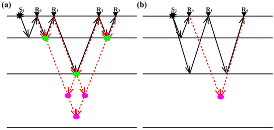
Figure 1.
Schematic diagrams of RTMM and crosstalks. The green points in panel (a) represent the imaging points. The magenta points in panels (a,b) represent the order-related and event-related crosstalks, respectively.
Crosstalk artifacts are sorted into two types, i.e., order-related crosstalks and event-related crosstalks [19]. Order-related crosstalks are caused by the interactions between inconsecutive-order multiples and comprise a major portion of crosstalks. All order-related crosstalks (magenta points in Figure 1a) compose the crosstalks term , as shown by Equation (6). In Figure 1a, the primary recorded at can be forward propagated and crosscorrelated with the backward-propagated second-order multiples recorded at or third-order multiples recorded at . Because the order difference between forward- and backward-propagated data is two or three, the interactions cause coherent order-related crosstalks, as denoted by the magenta points. Similarly, the first-order multiples recorded at can be treated as the secondary virtual sources of the third-order multiples recorded at , and the interaction between them also yields order-related crosstalk artifacts. When the migration is conducted by using consecutive-order multiple pairs (Equation (5)), such as the pair of forward-propagated primaries and backward-propagated first-order multiples, the imaging result is free of order-related crosstalks but retains event-related crosstalks. In the consecutive-order multiples pairs, seismic events can be classified into associated and unassociated multiple event pairs. The pair of associated multiple events is defined as a pair of multiples in which the backward-propagated higher-order multiple is equal to the convolution result between the forward-propagated lower-order multiple and the accurate impulse response from one special interface. The associated multiple events comply with the feedback model. On the contrary, the pair of unassociated events fail to meet the feedback model. According to the time-consistent principle, the crosscorrelations between associated multiple events retrieve an accurate image, whereas the interactions between unassociated multiple events create event-related crosstalks. Consequently, an accurate image, together with event-related crosstalks, comprises the useful term . As shown in Figure 1b, when the image is retrieved by backward penetrating the first-order multiple recorded at and forward penetrating the primary recorded at , the two multiples are unassociated, thereby resulting in event-related crosstalk, as indicated by the magenta point.
2.2. Multiples Decomposition Strategies
Crosstalk artifacts smear accurate subsurface imaging structures and severely hinder the practical applications of multiple imaging. To eliminate energetic order-related crosstalks, Liu et al. [20] separated multiples into different orders before migration in combination with RTMM to conduct controlled-order multiples imaging, which is referred to as RTM of controlled-order multiples (RTM-CM). The imaging condition of RTM-CM can be expressed by:
The comparison between Equations (5) and (7) reveals that RTM-CM is equal to the useful term of RTMM by exchanging the orders of the inner summations. By removing the crosstalk terms in the imaging condition, RTM-CM can effectively avoid order-related crosstalks, but still retain event-related crosstalk components, as shown in Figure 1b [19].
After the separation of primaries and multiples, RTMM can be accomplished by simultaneously forward propagating original data and backward propagating the estimated multiples. However, the regular SRME is unable to provide isolated-order multiples for RTM-CM. Therefore, we extend the regular SRME. Taking the matrix notation, the frequency-domain SRME can be formalized by:
where represents the original data matrix, represents the primaries matrix, represents the multiples matrix, and represents the surface operator. , where represents the maximum order, and represents the ith-order multiples. Equation (8) indicates that higher-order multiples are predicted by the time-domain convolutions between primaries and lower-order multiples. By extending the SMRE, the extraction of different-order multiples is given by:
where represents the matching filter, and represents a group of multiples with i as the minimum order. Taking the isolation of first-order multiples as an example, the primaries matrix is multiplied with the estimated multiples matrix () to generate the predicted data matrix , followed by adaptively subtracting from to obtain the estimated first-order multiples. Similarly, higher-order multiples can be effectively extracted by repeating the loops in Equation (9).
The consecutive-order multiples pair used in RTM-CM contains pairs of associated and unassociated events. The interaction between unassociated multiple events causes event-related crosstalks (Figure 1b). Therefore, we attempt to only extract the pairs of associated multiple events. Among strong multiples, such as the signals from the sea bottom or the salt boundaries, the water-column multiples bouncing in the water layer are easily simulated, and, by using the feedback model, the water-bottom-related multiples associated with water-column multiples can be obtained. The black ray paths and of Figure 2a represent the traveling routes of the water-column primary and first-order water-bottom-related multiple, respectively. The water-column primaries can be predicted by wave equation modeling [37,38,39] with a water layer model:
where represents the forward modeling operator, represents the water bottom reflectivity model, and represents the predicted water-column primaries. After adaptively matching with , we can acquire the estimated water-column primaries . The predicted nth-order water-column multiples are then obtained by the n times auto-convolutions of estimated water layer primaries:
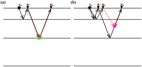
Figure 2.
Schematic diagrams of (a) RTM-WM and (b) residual crosstalks. The imaging point represented by the green point in panel (a) is created by the crosscorrelation between the forward-propagating water-column primaries and the backward-propagating first-order water-bottom-related multiples. The magenta point in panel (b) indicates the residual non-stationary crosstalks.
Subsequently, we adaptively match with to extract the estimated nth-order water-bottom-related multiples . By multiplying with (), we can gain the predicted (n+1)th-order water-bottom-related multiples , followed by adaptively matching with to extract the estimated . For example, assigning n = 0, the water-column primaries are obtained using Equation (10), and the predicted first-order water-bottom-related multiples are then acquired by convolving the water-column primaries with the primaries . Finally, we adaptively match the predicted first-order water-bottom-related multiples with the original data to extract the estimated first-order water-bottom-related multiples .
2.3. Least-Squares Reverse-Time Migration of Water-Bottom-Related Multiples
Following Zhang et al. [19], the imaging condition (Equation (7)) of RTM-CM can be expanded into:
where represents the wavefield with the nth-order water-column multiples as sources, represents the wavefield with residual nth-order multiples as sources, represents the backward-propagated (n+1)th-order water-bottom-related multiples wavefield, and represents the residual backward-propagated (n+1)th-order water-bottom-related multiples wavefield. As the nth-order water-column multiples are associated with the (n+1)th-order water-bottom-related multiples but unassociated with the remaining (n+1)th-order multiples, is strictly associated with but unassociated with . Likewise, is unassociated with , and it contains associated and unassociated components with . Therefore, we expand Equation (12) into three parts, as shown in Equation (13):
where is the accurate imaging term for water-bottom-related multiples, is the mixed term containing accurate imaging results and event-related crosstalks, and is the crosstalks term consisting of event-related crosstalks. To avoid event-related crosstalks, Zhang et al. [19] only reserved in the imaging condition and developed the reverse-time migration of water-bottom-related multiples (RTM-WM) in which the nth-order water-column multiples are forward propagated, and the (n+1)th-order water-bottom-related multiples are backward propagated (see Figure 2a). Compared with RTM-CM, RTM-WM simplifies the propagated wavefield and utilizes the associated multiples, thereby effectively suppressing event-related crosstalks. Nevertheless, as indicated by the magenta point in Figure 2b, the crosscorrelations between unrelated multiples in associated multiples pairs cause non-stationary crosstalks, and the crosstalks are random and can significantly cancel each other out due to destructive interference.
Least-squares reverse-time migration (LSRTM) has been extensively investigated to eliminate imaging artifacts, improve spatial resolution, and balance imaging amplitudes. Combining LSRTM with RTMM, the LSRTM of multiples (LSRTMM) has been proposed to mitigate serious multiples crosstalks. Unlike LSRTM, LSRTMM builds a reflectivity model that minimizes the objective function between the observed and predicted multiples. The predicted multiples are generated by Born modeling with the original data as virtual sources, and the observed multiples are separated using the regular SRME. As RTMM or RTM-CM produces images with coherent crosstalks and is used as the gradient engine, the predicted multiples contain numerous undesired data events, thereby resulting in poor convergence of the objective function and inadequate crosstalk removal.
As RTM-WM can significantly eliminate crosstalks and provide better gradients for least-squares inversion than RTMM and RTM-CM, we propose the LSRTM of water-bottom-related multiples (LSRTM-WM) to enhance the imaging quality. Similar to the Born modeling associated with multiples, the Born modeling associated with (i+1)th-order water-bottom-related multiples can be established by replacing the original data with ith-order water-column multiples:
where represents the reflectivity model, represents the forward-propagated background wavefield excited by the ith-order water-column multiples , represents the scattering wavefield, and represents the predicted (i+1)th-order water-bottom-related multiples. Equation (15) can be rewritten in a short form by:
where is the Born modeling operator associated with (i+1)th-order water-bottom-related multiples. To produce a satisfied reflectivity, the difference between the observed and predicted (n+1)th-order water-bottom-related multiples can be minimized using the following objective function:
where represents the observed (n+1)th-order water-bottom-related multiples. To figure out the minimization problem, we use a preconditioned conjugate gradient method in the following manner:
where indicates the gradient of the objective function in Equation (17), represents the migration operation, denotes the source-side illumination compensation, and z is the iteration number.
2.4. LSRTM-WM Scheme
- (1)
- Separate primaries from original data using Equation (8) and predict water-column primaries using Equation (10);
- (2)
- Auto-convolve the water-column primaries n times to generate the nth-order water-column multiples using Equation (11), followed by convolutions between the nth-order water-column multiples and the separated primaries to obtain the (n+1)th-order water-bottom-related multiples;
- (3)
- Set the initial reflectivity model to zero;
- (4)
- Establish the objective function using Equation (17);
- (5)
- Calculate the gradients for the objective function and update the reflectivity model using Equation (18);
- (6)
- Repeat steps 4 to 5 and stop the iterative inversion when the objective function decreases to a given threshold;
- (7)
- Stack different-order (from first to N-th) images to retrieve the final image of water-bottom-related multiples.
3. Numerical Examples
In this section, we verify the feasibility of LSRTM-WM using a layered model and then utilize the Pluto 1.5 model to confirm the effectiveness and benefits of LSRTM-WM for imaging complex structures. Together with the apparent fact that the first-order multiples are generally more energetic than higher-order multiples, the LSRTM-WM was implemented on the associated multiple pair of water-column primaries and first-order water-bottom-related multiples in this study. Under the circumstances, Equation (17) can be adjusted to:
where represents the Born modeling operator with the water-column primaries as incident wavefield, and is the observed first-order water-bottom-related multiples.
3.1. A Layered Model
We first implemented the proposed approach on a five-layer velocity model, as shown in Figure 3. The model was discretized into 801 horizontal grids and 451 vertical grids both with a 5 m spatial interval. There were three flat interfaces and one curved interface. The split-spread geometry and a Ricker wavelet with a 20 Hz dominant frequency were selected to produce seismic data. There were 96 shot gathers used for migration. The first shot was fixed at 0.81 km, and the shot interval was 25 m. Each shot gather involved 301 traces with a 5 m receiver interval. The recording length was 3.92 s, and the time sampling rate was 8 ms. The water-column primaries were simulated by wave equation modeling with the water (first) layer velocity model.
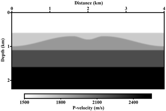
Figure 3.
The layered velocity model.
After the separation of primaries and multiples using regular SRME, we investigated conventional LSRTM and LSRTMM. The LSRTM algorithm with six iterations was first conducted to retrieve a crosstalk-free image, as shown in Figure 4a. The primary image was treated as the benchmark to examine the performances of multiples in imaging. Figure 4b shows the migration result of LSRTMM. As RTMM introduced severe crosstalks and was treated as the modeling and migration engine, LSRTMM suppressed crosstalks unsatisfactorily, as shown by the black arrows in Figure 4b. To eliminate the artifacts caused by crosstalks, we applied RTM-WM, and the resulting image was as shown in Figure 5a. Based on the feedback model, we extracted the first-order water-bottom-related multiples by convolving the predicted water-column primaries with estimated primaries. By forward propagating the water-column primaries and backward propagating the associated first-order water-bottom-related multiples, RTM-WM effectively reduced almost all crosstalks (indicated by the black arrows in Figure 5a). Compared with the LSRTM and LSRTMM results, the RTM-WM result exhibited a lower spatial resolution. To settle this problem and enhance imaging quality, the developed LSRTM-WM was then used. Figure 5b is the least-squares image based on the image shown in Figure 5a. As shown in Figure 6, a further comparison between RTM-WM and the developed LSRTM-WM was executed by the wavenumber spectra. The LSRTM-WM image presented significantly broader spectrum components than the RTM-WM image. Moreover, the comparison between Figure 5b against Figure 4a,b revealed that LSRTM-WM can remove crosstalks more effectively than LSRTMM and retrieve an image with a high signal-to-noise ratio (SNR), as is quite similar to LSRTM. This model test verified the feasibility of the proposed method and its advantages over LSRTMM in terms of crosstalk noise suppression.
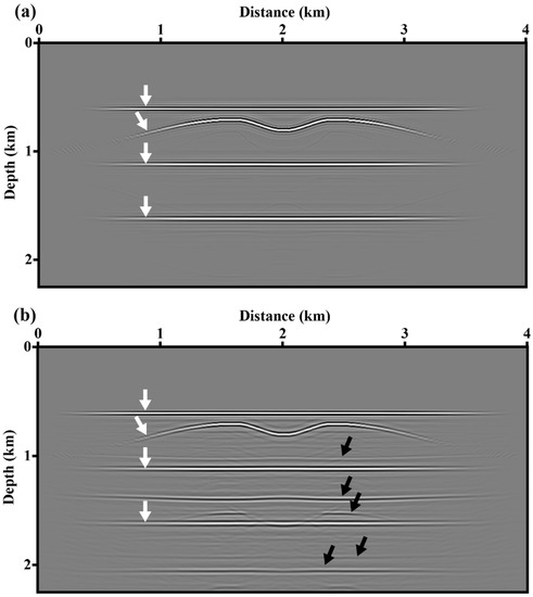
Figure 4.
(a) The LSRTM image and (b) the LSRTMM image. Both images were produced after six iterations. The white arrows in panels a and b illustrate that both LSM algorithms imaged the four interfaces well. As shown by the black arrows in panel b, LSRTMM exhibited a poor capacity to suppress crosstalks generated by undesired multiples crosscorrelations.
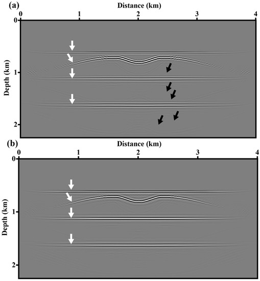
Figure 5.
(a) The RTM-WM image and (b) the LSRTM-WM (six iterations) image.
3.2. The Pluto 1.5 Model
The 2D Subsalt Multiples Attenuation and Reduction Team (SMAART) Pluto 1.5 model shown in Figure 7 was subsequently used to validate the performance of our approach in imaging complex structures. The model contained 1387 grids with a 22.86 m grid spacing along the horizontal direction and 1201 grids with a 7.62 m grid spacing along the vertical direction. The source wavelet was a Ricker wavelet with a 25 Hz peak frequency. A total of 232 shots with a shot interval of 137.16 m were evenly organized from 0 km to 31.7 km. The sources and receivers were located at a depth of 7.62 m. Each shot gather possessed 540 traces with a geophone interval of 22.86 m. The recording length and time sampling interval were 9 s and 8 ms, respectively. A water layer velocity model, in which the velocity under the water bottom was set to 4512.20 m/s (the salt velocity), was used to produce pronounced water-column primaries.
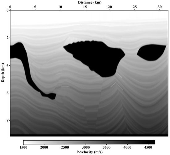
Figure 7.
Pluto 1.5 velocity model.
Figure 8 shows the separated results of different orders using the multiples decomposition strategy. First, we separated the primaries (Figure 8b) and multiples (Figure 8c) from the original data (Figure 8a) using regular SRME. As indicated by the arrows in Figure 8b, multiples were well attenuated in the estimated primaries. Subsequently, the primaries were convolved with multiples to predict multiples with a minimum order of 2, followed by adaptively subtracting them from all-order multiples (Figure 8c) to obtain the isolated first-order multiples. The resulting first-order multiples were as shown in Figure 8d. By using the decomposition workflow, the higher-order multiples, as indicated by the black arrows in Figure 8d, were well avoided, and the first-order multiples, as denoted by the white arrows in Figure 8d, remained. The convolution between the predicted water-column primaries and the separated primaries in Figure 8b was conducted to predict the first-order water-bottom-related multiples. By adaptively matching the predicted data with the original data, we extracted the estimated first-order water-bottom-related multiples (Figure 8e). As demonstrated by the red arrows in Figure 8e, the multiples unassociated with the water-column primaries were well removed. The complex multiples extraction strongly corroborated the effectiveness of the decomposition strategy in separating different-order multiples.
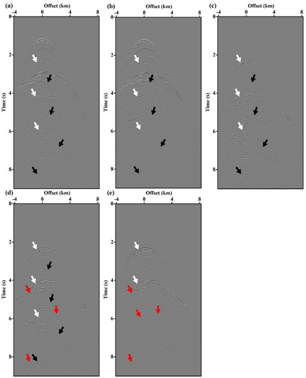
Figure 8.
Multiples decomposition results for Pluto 1.5 model. (a) One original gather, (b) separated primaries, (c) all-order multiples, (d) first-order multiples, and (e) first-order water-bottom-related multiples. The white, black, and red arrows indicate the first-order multiples, higher-order multiples, and multiples unassociated with the water-column primaries, respectively.
After the decomposition of different-order multiples, different migration algorithms were conducted. Applying conventional LSRTM (six iterations) to the separated primaries (Figure 8b) resulted in the image in Figure 9a. Note that we had muted crosstalks in the water layer and considered the LSRTM result as the reference for the following analysis. By forward propagating the original data (Figure 8a) and backward propagating the estimated multiples (Figure 8c), we accomplished the LSRTMM, and Figure 9b shows the imaging result after six iterations. The sedimentary layers, salt boundaries, and dipping faults were well depicted, whereas the crosstalks caused by RTMM were not thoroughly suppressed by LSRTMM. The residual crosstalks masked the true strata and may trigger wrong geological interpretations. For example, the crosstalk pointed by the upper five arrows in Figure 9b was approximately parallel to the seafloor, and it was prone to be recognized as a bottom-simulating reflector (a robust geophysical indicator for the presence of gas hydrate). To remove crosstalk artifacts, we implemented RTM-WM by forward propagating the water-column primaries and simultaneously backward propagating the first-order water-bottom-related multiples (Figure 8e), and the resulting image was as shown in Figure 10a. Compared with the LSRTMM (Figure 9b), RTM-WM significantly attenuated almost all crosstalks (see the arrows) and exhibited a higher SNR. Further, we employed the RTM-WM as the modeling and migration engine and applied the proposed LSRTM-WM. Figure 10b shows the LSRTM-WM result after six iterations. The comparison between Figure 10a,b reveals that the LSRTM-WM can effectively enhance imaging quality by improving spatial resolution. The comparison between Figure 9b and Figure 10b shows that LSRTM-WM can effectively remove the residual crosstalks which were partially reduced by the LSRTMM. Moreover, the SNR shown in Figure 10b was quite similar to that of the conventional LSRTM image using primaries shown in Figure 9a.

Figure 9.
(a) The LSRTM (six iterations) image and (b) the LSRTMM (six iterations) image.
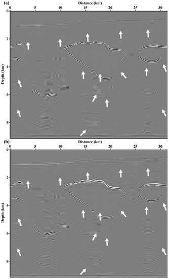
Figure 10.
(a) The RTM-WM image and (b) the LSRTM-WM (six iterations) image.
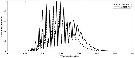
In conventional least-squares inversions, in addition to the accurate migration velocity model, wavelet estimation is another vital task for seismic data processing, especially for field dataset processing. If the estimated wavelet is far from the accurate one, the convergence of the objective function for LSRTM slowly decreases and even increases. However, in the imaging of multiples, we treat the seismic data, rather than a point source wavelet, as the virtual sources at each receiver. Therefore, the imaging of multiples is independent of wavelet estimation and robustly produces imaging results. In this experiment, we designed a comparison to investigate the performances of different migration algorithms when the wavelet is inaccurately estimated. We assumed that the dominant frequency of the wavelet was 7 Hz and conducted LSRTM of primaries. The LSRTM image with the inaccurate wavelet after six iterations was as shown in Figure 11. Among all the least-squares images above (Figure 9a,b, Figure 10b and Figure 11), the LSRTM image using the inaccurate wavelet was the worst one and exhibited a lower wavenumber feature. This was due to the used 7 Hz dominant frequency being smaller than the true 15 Hz dominant frequency. Figure 12 displays the convergence curves for the LSRTM (the black line), the proposed LSRTM-WM (the red line), and the LSRTM with the inaccurate wavelet (the green line). Both the objective functions of LSRTM and LSRTM-WM quickly decreased as the iterations increased, whereas the objective function of LSRTM with the inaccurate wavelet slowly decreased. Notably, the misfit function for LSRTM consistently achieved a faster convergence than that of LSRTM-WM. This may have been driven by the fact that there were residual unassociated multiples. The convergence comparisons reveal that LSRTM-WM may robustly produce higher-quality images than LSRTM in some field data processing. Moreover, as multiples undergo several bounces beneath the free surface, multiples contain wider wavenumber components than corresponding primaries [40,41]. To further emphasize the advantages of imaging using multiples, we compared the wavenumber spectra of the different images in Figure 13 (the dashed black line represents the RTM-WM image in Figure 10a, the solid black line is the LSRTM-WM image in Figure 10b, the solid blue line denotes the LSRTM image in Figure 9a, and the solid red line represents the LSRTM image in Figure 11 with the inaccurate wavelet). Compared with the images of primaries (the red and blue lines), the images of multiples (the black lines) exhibited significantly broader wavenumber spectra. As indicated by the red line, the wavenumber spectrum of the LSRTM image with the inaccurate wavelet was biased toward the lower wavenumber components. This was caused by the usage of a lower dominant frequency for least-squares inversion. The comparison between the dotted and solid black lines indicates that the LSRTM-WM can more effectively broaden the wavenumber spectra than RTM-WM. As the wavenumber spectra can represent the resolution along the depth direction to some extent, LSRTM-WM retrieves images with higher resolution than RTM-WM.
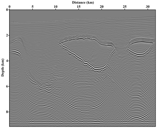
Figure 11.
The LSRTM (six iterations) image with the inaccurate wavelet.
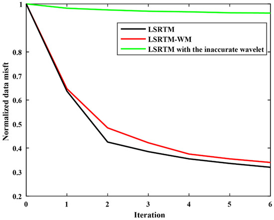
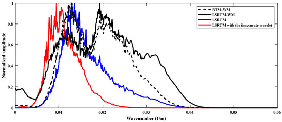
Figure 13.
Wavenumber spectra comparison in the depth direction for different migration images. The dashed black, solid black, solid blue, and solid red lines represent the wavenumber spectra for images from RTM-WM (Figure 10a), LSRTM-WM (Figure 10b), LSRTM (Figure 9a), and LSRTM with the inaccurate wavelet (Figure 11), respectively.
4. Conclusions
A new least-squares reverse-time migration of water-bottom-related multiples (LSRTM-WM) was developed to attenuate crosstalks and enhance imaging quality. In the proposed approach, SRME, combined with the feedback model, is exploited to separate multiples into different orders, and RTM-WM is recognized as the forward modeling and migration engine. Compared to RTM-WM, LSRTM-WM can produce an image with a better signal-to-noise ratio, higher spatial resolution, and more balanced amplitudes. Furthermore, LSRTM-WM can effectively eliminate both the order-related and event-related crosstalks which are partially reduced by LSRTMM. In addition, as multiples bounce several rounds in the subsurface, the LSRTM-WM image can recover broader wavenumber components than that of LSRTM using primaries. Moreover, for the usage of seismic data as the secondary virtual sources, LSRTM-WM is independent of seismic wavelets and can robustly retrieve an imaging result that is quite similar to that of LSRTM with the accurate wavelet. Numerical experiments demonstrated the effectiveness and advantages of the proposed method and verified that the LSRTM-WM is a promising algorithm for imaging complex marine structures.
Author Contributions
Conceptualization, Y.Z. and Y.L.; methodology, Y.Z.; software, J.Y.; formal analysis, Y.Z.; investigation, J.Y.; resources, Y.L.; writing—original draft preparation, Y.Z.; writing—review and editing, Y.L. and J.Y.; supervision, Y.L. All authors have read and agreed to the published version of the manuscript.
Funding
The research was co-funded by the National Natural Science Foundation of China (grant numbers 42104114 and 42130807) and the Open Fund of State Key Laboratory of Geodesy and Earth’s Dynamics, Innovation Academy for Precision Measurement Science and Technology, Chinese Academy of Sciences (grant number SKLGED2022-5-3).
Data Availability Statement
The data used in this study are available through contacting the corresponding author.
Acknowledgments
We would like to acknowledge the SMAART JV consortium for the synthetic Pluto 1.5 velocity model and dataset.
Conflicts of Interest
The authors declare no conflict of interest.
References
- Brown, M.; Guitton, A. Least-squares joint imaging of multiples and primaries. Geophysics 2005, 70, S79–S89. [Google Scholar] [CrossRef]
- Muijs, R.; Robertsson, J.; Holliger, K. Prestack depth migration of primary and surface-related multiple reflections: Part I-Imaging. Geophysics 2007, 72, S59–S69. [Google Scholar] [CrossRef]
- Zuberi, A.; Alkhalifah, T. Imaging by forward propagating the data: Theory and application. Geophys. Prospect. 2013, 61, 248–267. [Google Scholar] [CrossRef]
- Wapenaar, K.; Thorbecke, J.; van ver Neut, J.; Broggini, F.; Slob, E.; Snieder, R. Marchenko imaging. Geophysics 2014, 79, WA39–WA57. [Google Scholar] [CrossRef]
- Liu, Y.K.; Zhu, W.L.; Mi, L.J.; Zhou, J.X.; Hu, H. Migration of multiples from the South China Sea. Sci. China Earth Sci. 2015, 58, 482–490. [Google Scholar] [CrossRef]
- Lu, S.P.; Whitmore, D.; Valenciano, A.; Chemingui, N. Separated-wavefield imaging using primary and multiple energy. Lead Edge 2015, 34, 770–778. [Google Scholar] [CrossRef]
- Zheng, Y.K.; Wang, Y.B.; Xu, J.L.; Chang, X.; Yao, Z.X. Imaging multiples by data to data migration. Chin. J. Geophys. 2015, 58, 993–1001. [Google Scholar] [CrossRef]
- Liu, X.J.; Liu, Y.K.; Hu, H.; Li, P.; Khan, M. Imaging of first-order surface-related multiples by reverse-time migration. Geophys. J. Int. 2017, 208, 1077–1087. [Google Scholar] [CrossRef]
- Liu, Y.K.; He, B.; Zheng, Y.C. Controlled-order multiple waveform inversion. Geophysics 2020, 85, R243–R250. [Google Scholar] [CrossRef]
- Mäkinen, A.; Rickett, J.; Kostov, C. Free-surface multiples least-squares RTM with unrecorded data compensation applied to marine 3D field data. In EAGE Annual Conference & Exhibition; European Association of Geoscientists & Engineers: Houten, The Netherlands, 2020; pp. 1–5. [Google Scholar] [CrossRef]
- Zhang, Y.B.; Liu, Y.K.; Yi, J.; Liu, X.J. First-order multiples imaging aided by water bottom. Pet. Sci. 2021, 18, 1650–1661. [Google Scholar] [CrossRef]
- Liu, Y.K.; Zhang, Y.B.; Zheng, Y.C. Reverse time migration of phase-encoded all-order multiples. Geophysics 2022, 87, S45–S52. [Google Scholar] [CrossRef]
- Guitton, A. Shot-profile migration of multiple reflections. In 72nd SEG Technical Program Expanded; Society of Exploration Geophysicists: Houston, TX, USA, 2002; pp. 1296–1299. [Google Scholar] [CrossRef]
- Jiang, Z.Y.; Sheng, J.M.; Yu, J.H.; Schuster, G.T.; Hornby, B.E. Migration methods for imaging different-order multiples. Geophys. Prospect. 2007, 55, 1–19. [Google Scholar] [CrossRef]
- Verschuur, D.; Berkhout, A. Transforming multiples into primaries: Experience with field data. In 75th SEG Technical Program Expanded; Society of Exploration Geophysicists: Houston, TX, USA, 2005; pp. 2103–2106. [Google Scholar] [CrossRef]
- Verschuur, D.; Berkhout, A.; Wapenaar, C. Adaptive surface-related multiple elimination. Geophysics 1992, 57, 1166–1177. [Google Scholar] [CrossRef]
- Liu, Y.K.; Chang, X.; Jin, D.G.; He, R.Q.; Sun, H.C.; Zheng, Y.C. Reverse time migration of multiples for subsalt imaging. Geophysics 2011, 76, WB209–WB216. [Google Scholar] [CrossRef]
- Berkhout, A.; Verschuur, D. Multiple technology: Part 2, Migration of multiple reflections. In 64th SEG Technical Program Expanded; Society of Exploration Geophysicists: Houston, TX, USA, 1994; pp. 1497–1500. [Google Scholar] [CrossRef]
- Zhang, Y.B.; Liu, Y.K.; Liu, X.J.; Zhou, X.P. Reverse time migration using water-bottom-related multiples. Geophys. Prospect. 2020, 68, 446–465. [Google Scholar] [CrossRef]
- Liu, Y.K.; Liu, X.J.; Osen, A.; Shao, Y.; Hu, H.; Zheng, Y.C. Least-squares reverse time migration using controlled-order multiple reflections. Geophysics 2016, 81, S347–S357. [Google Scholar] [CrossRef]
- Berkhout, A. Multiple removal based on the feedback model. Lead Edge 1999, 18, 127–131. [Google Scholar] [CrossRef]
- Nemeth, T.; Wu, C.J.; Schuster, G. Least-squares migration of incomplete reflection data. Geophysics 1999, 64, 208–221. [Google Scholar] [CrossRef]
- Dai, W.; Fowler, P.; Schuster, G. Multi-source least-squares reverse time migration. Geophys. Prospect. 2012, 60, 681–695. [Google Scholar] [CrossRef]
- Luo, S.; Hale, D. Least-squares migration in the presence of velocity errors. Geophysics 2014, 79, S153–S161. [Google Scholar] [CrossRef]
- Zhang, Y.; Duan, L.; Xie, Y. A stable and practical implementation of least-squares reverse time migration. Geophysics 2015, 80, V23–V31. [Google Scholar] [CrossRef]
- Liu, X.J.; Liu, Y.K.; Lu, H.Y.; Hu, H.; Khan, M. Prestack correlative least-squares reverse time migration. Geophysics 2017, 82, S159–S172. [Google Scholar] [CrossRef]
- Yang, K.; Zhang, J.F. Least-squares reverse time migration with an angle-dependent weighting factor. Geophysics 2018, 83, S299–S310. [Google Scholar] [CrossRef]
- He, B.; Liu, Y.K.; Zhang, Y.B. Improving the least-squares image by using angle information to avoid cycle skipping. Geophysics 2019, 84, S581–S598. [Google Scholar] [CrossRef]
- Fang, J.W.; Zhou, H.; Chen, H.M.; Wang, N.; Wang, Y.F.; Sun, P.Y.; Zhang, J.L. Source-independent elastic least-squares reverse time migration. Geophysics 2019, 84, S1–S16. [Google Scholar] [CrossRef]
- Li, C.; Gao, J.H.; Gao, Z.Q.; Wang, R.R.; Yang, T. Periodic plane-wave least-squares reverse time migration for diffractions. Geophysics 2020, 85, S185–S198. [Google Scholar] [CrossRef]
- Mao, W.J.; Duan, W.G.; Sun, C.X.; Shi, X.C. Elastic least-squares gaussian beam imaging with point spread functions. IEEE Geosci. Remote Sens. Lett. 2022, 19, 1–5. [Google Scholar] [CrossRef]
- Wong, M.; Biondi, B.; Ronen, S. Imaging with primaries and free-surface multiples by joint least-squares reverse time migration. Geophysics 2015, 80, S223–S235. [Google Scholar] [CrossRef]
- Liu, X.J.; Liu, Y.K. Plane-wave domain least-squares reverse time migration with free-surface multiples. Geophysics 2018, 83, S477–S487. [Google Scholar] [CrossRef]
- Liu, X.J.; Liu, Y.K.; Khan, M. Fast least-squares reverse time migration of VSP free-surface multiples with dynamic phase-encoding schemes. Geophysics 2018, 83, S321–S332. [Google Scholar] [CrossRef]
- Zheng, Y.K.; Wang, Y.B.; Chang, X. Least-squares data-to-data migration: An approach for migrating free-surface-related multiples. Geophysics 2019, 84, S83–S94. [Google Scholar] [CrossRef]
- Nocedal, J.; Wright, S. Numerical Optimization; Springer Science and Business Media: Berlin, Germany, 2006. [Google Scholar]
- Alford, R.; Kelly, K.; Boore, D. Accuracy of finite-difference modeling of the acoustic wave equation. Geophysics 1974, 39, 834–842. [Google Scholar] [CrossRef]
- Gao, Y.J.; Song, H.J.; Zhang, J.H.; Yao, Z.X. Comparison of artificial absorbing boundaries for acoustic wave equation modelling. Explor. Geophys. 2017, 48, 76–93. [Google Scholar] [CrossRef]
- Wang, N.; Xing, G.; Zhu, T.Y.; Zhou, H.; Shi, Y. Propagating seismic waves in VTI attenuating media using fractional viscoelastic wave equation. J. Geophys. Res. Solid Earth 2022, 127, e2021JB023280. [Google Scholar] [CrossRef]
- Tu, N.; Herrmann, F. Fast least-squares imaging with surface-related multiples: Application to a North Sea data set. Lead Edge 2015, 34, 788–794. [Google Scholar] [CrossRef]
- Li, Z.N.; Li, Z.C.; Li, Q.; Li, Q.; Sun, M.; Hu, P.; Li, L. Least-squares reverse time migration of multiples in viscoacoustic media. Geophysics 2020, 85, S285–S297. [Google Scholar] [CrossRef]
Publisher’s Note: MDPI stays neutral with regard to jurisdictional claims in published maps and institutional affiliations. |
© 2022 by the authors. Licensee MDPI, Basel, Switzerland. This article is an open access article distributed under the terms and conditions of the Creative Commons Attribution (CC BY) license (https://creativecommons.org/licenses/by/4.0/).
