Abstract
This paper provides a general formularization of the nonlocal Euler–Bernoulli nanobeam model for a bending examination of the symmetric and asymmetric cross-sectional area of a nanobeam resting over two linear elastic foundations under the effects of different forces, such as axial and shear forces, by considering various boundary conditions’ effects. The governing formulations are determined numerically by the Generalized Differential Quadrature Method (GDQM). A deep search is used to analyze parameters—such as the nonlocal (scaling effect) parameter, nonuniformity of area, the presence of two linear elastic foundations (Winkler–Pasternak elastic foundations), axial force, and the distributed load on the nanobeam’s deflection—with three different types of supports. The significant deductions can be abbreviated as follows: It was found that the nondimensional deflection of the nanobeam was fine while decreasing the scaling effect parameter of the nanobeams. Moreover, when the nanobeam is not resting on any elastic foundations, the nondimensional deflection increases when increasing the scaling effect parameter. Conversely, when the nanobeam is resting on an elastic foundation, the nondimensional deflection of the nanobeam decreases as the scaling effect parameter is increased. In addition, when the cross-sectional area of the nanobeam varies parabolically, the nondimensional deflection of the nonuniform nanobeam decreases in comparison to when the cross-sectional area varies linearly.
1. Introduction
Structural analysis is an overall computation of the load applied to the structure to emphasize that the distortions due to the load on a structure will be satisfying and reach the minimal permissible limits, and to ensure that structure failure will never occur. Analytical results are employed to confirm the structure’s strength for use. So, structural analysis is a basic part of structural engineering. A bending study is useful for some engineering applications such as some types of sensors and bows and arrows. The purpose of structural analysis from its solidity standpoint is the determination of the bending at particular points of a structure in accordance with the external forces, since bending considers the most common reason for structural failures in bridges, blades, and shafts too. Any system needs a careful analysis of bending properties for design and validation processes. So, the bending that occurs should always be controlled and monitored. Studying the reasons and factors affecting deflection helps us to adequately control the system. Therefore, it is necessary to compare the occurrence of deflection with the critical deflection of the system, or failures will occur. This dilemma has attracted many members of the scientific community to studying the characteristics of structural bending for extremely varied cases such as beams, plates, rings, shells, wires, and any other possible shapes.
The invention of carbon nanotubes [1] attracted researchers and manufacturers to the use of this substance in highly accurate studies and industries. A new revolution has begun in all the fields of the industry due to the properties of new nanomaterials. Studying these properties in labs is highly expensive and complicated because of the strict conditions of the purity of the material, air, tools, and everything related to this process. Consequently, a new role in mathematics was initiated, concerning the study of such properties with low costs.
Mathematical researchers started to use different theories to describe beams. Beams have been studied in accordance with the Euler–Bernoulli [2,3,4,5,6], Timoshenko [7,8,9], Reddy [8,10], and Levinson beam theories [10].
The fourth-order ordinary differential equations in the Euler–Bernoulli theorem, which is not normally combined with linear analysis, are now conjugated and must be overcome to obtain an acceptable mathematical solution of the axial deformation and the transverse rotation of thin beams. The axial force that can be produced inside the beam tries to firm up the beam when it deforms.
In old-fashioned classical continuum mechanics studying beams, the stress at a point depends on the strains for the same point. Poor results have appeared after applying those methods to nanobeams because of the attraction forces between molecules and crystals. This phenomenon is called the size effect. The mathematical process of analyzing nanostructures is divided into three main types. The first of them is atomistic modeling [11]. The second and most used method is that of modern continuum mechanics. Finally, the last one is a mixture of atomistic and continuum mechanics. The highly accurate results of continuum models can be found in improved elasticity theories such as Eringen’s nonlocal elasticity theory. Refs. [12,13] are the most common examples in this field. Ref. [12] assumed that a point’s stress depends on deformations of the whole continuum.
One of the important factors affecting the deformation properties of beams is the foundation on which the beam rests or the medium around the beam. The density of the medium causes a buoyant force that affects the beam’s upward characteristics. Foundations are used also to control and change the deformation of the loaded beam depending on the application in which the beam is being used. Several types of elastic and viscoelastic foundation theories have been derived, such as the Winkler model, the Filonenko–Borodich Foundation, the Hetenyi Foundation, the Pasternak Foundation, the Vlasov Foundation, the Reissner Foundation, and Boussinesq’s type foundation [14]. Winkler’s foundation is described as a single parameter model similar to a liquid base or a net of equally-spaced equivalent springs, but Pasternak’s foundation is a double-parameter model which adds the effect of shear interactions inside every spring. The applications of elastic foundations supporting beams are several, including geotechnical systems, roads, railroads, and biomechanical systems.
The applications of microbeams and nanobeams are always complex and require high accuracy. This can be obviously noted in [15], which deduced the vibration and post-buckling of bi-directional functionally graded microbeams; Ref. [16], which studied nano composites; Ref. [17], which showed the effect of temperature on nanobeams; Ref. [18], which studied piezomagnetic nanobeams with porosities; Ref. [19], which studied flexoelectric nanobeams’ dynamics; Ref. [17], which focused on the thermal effects on nanobeam properties; and [20], which analyzed layered nanobeams. The complexity of the equations covering several factors prompted many researchers to use some semi-analytical and numerical methods instead of strictly analytical solutions—such as the Finite Element Method (FEM), Finite Difference Method (FDM), Transfer Matrix Method, Rayleigh–Ritz Method, Galerkin Procedure, Differential Transform Method, and Differential Quadrature Method (DQM)—to resolve these types of models. When the analytical solution of irregular beams or plates requires solving differential equations with inconstant coefficients, hard work necessarily follows. Most numerical methods need an enormous number of mesh points to supply highly delicate results such as the classical techniques (FEM and FDM). Unfortunately, in some realistic models, the numeral solutions for governing equations are needed at a few specific points in the naturalistic scope. In searching for an alternative numerical technique utilizing a few mesh points to reach acceptable accuracy results, the DQM was inserted as the efficacy technique by [21]; then, it was improved by [22]. The DQM was created to overcome the challenge of the long solution times required by computers to solve this type of equation via FEM with the same accuracy.
At first, the DQM was used to solve second-order differential equations such as nonlinear diffusion equations [23,24]. Refs. [25,26,27,28] widened the method to solve transport processes, the Poisson equation, multidimensional problems, the Thomas–Fermi equation, the pool boiling process in cavities, and the integrodifferential equation. The DQM was used for mechanical structures by Jang et al. [29], Wang et al. [2], and Bert et al. [30] to determine the deflection and buckling of different types of beams, plates, and columns. One of the greatest modifications of the DQM is the GDQM developed by Quan and Chang in two consecutive papers [31,32]. In these studies, the GDQM solved various initial-value equations. The GDQM was qualified for solving fourth-order partial differential equations with higher accuracy and was widened to several fields such as fluids [33,34,35], thermal energy storage [36], and structures [37,38,39,40,41,42]. New competitive fields in which the GDQM could be introduced to cover are microelectromechanical systems [43] and nanostructures [44,45,46]. The GDQM has been used successfully in our team’s work for solutions of a variety of applications such as in fluid mechanics [47,48] and structural analysis [40,41,42]. So, the GDQM has shown high efficiency in competitive fields.
Out of all the previously mentioned research directions, we were motivated to generalize a formulation studying the effect of influencing factors—as many as possible—on nanobeam bending with the intention for this research to be followed by further studies covering nanobeams, nanoplates, nanoshells, and nanosystems. The intention is to provide accurate formulations and equations regarding every part needed in nanomachines and nanorobots statically and dynamically.
This study aims to present three targets. The first target is to derive the general formularization of a nonlocal Euler–Bernoulli nonuniform loaded nanobeam via transverse and axial loads resting on two linear elastic foundations (Winkler and Pasternak models), and without neglecting the elastic effect of the deformation between the rings of each spring by considering three different types of boundary conditions. Euler–Bernoulli beam theory is utilized to describe the nanobeam with the size effect assumption of the nonlocal elasticity theory developed by Eringen. The next target is to use the GDQ technique to find the expected bending of uniform and nonuniform nanobeams as a result of the effective loads. In addition, the last target is to study and demonstrate the effectiveness of the varying cross-sectional area on the bending in different cases of elastic foundations and sets of boundary conditions.
2. Problem Formulation and Mathematical Formularization
2.1. Problem Formulation
2.1.1. Nonlocal Elasticity Theory
According to nonlocal elasticity theory, the nonlocal stress tensor at a point x is expressed as [49]
where
—the classical stress tensor at a point ;
—the nonlocal modulus (Kernel function);
—Euclidean distance;
—a material constant that depends on both internal and external characteristic lengths (scaling effect parameter).
Using Hooke’s law:
where
C—is the 4th order elasticity tensor;
ϵ—the classical strain tensor;
(:)—expresses the double dot product.
Equation (1) is a constitutive integration that is complicated to solve. An alternative differential relation is written as [49]
where
—Laplace operator;
—a constant measured by experiments and depends on the material;
a—lattice parameter;
L—the external characteristic length;
—the nonlocal parameter that expresses the size effect.
2.1.2. Euler–Bernoulli Beam Theory and Its Formulation
The coordinates are considered in the direction of the main three dimensions of the beam. In all beam theories, the geometry is such that the displacements along with the (x, y, z) coordinates are only functions of x and z coordinates and time t. Time functions are ignored in the case of calculating the maximum deflection. An Euler–Bernoulli beam has three main assumptions for its design. First of all, the plane sections are perpendicular to the neutral axis before deformation and stay planar and perpendicular to the neutral axis after deformation. Secondly, the deformations must be in a small range to ensure that they are under the elastic limit of the material without exceeding the yield stress of the material. Third, the cross-sectional area of the beam is assumed to be rigid as a result of ignoring Poisson’s ratio’s effects.
In [50], the displacement fields are described as:
where
u1—the displacement along the direction of length x;
u2—the displacement along the direction of width y;
u3—the displacement along the direction of thickness z;
w—the transverse displacement of the point (x, 0) on the mid-plane (z = 0);
t—time.
The relation between normal strain and displacement is described as: .
V—the shear force;
—the transverse distributed load affecting the beam;
—the different types of forces caused by the elastic foundation.

Figure 1.
The geometry of nonuniform beams on an elastic foundation under axial and transverse distributed loads.
Figure 1.
The geometry of nonuniform beams on an elastic foundation under axial and transverse distributed loads.

From Equations (6) and (9). This equation can be derived as:
From [10], the nonlocal constitutive relation is derived from the Euler–Bernoulli beam theory with Eringen’s nonlocal elasticity theory:
where
—the nonlocal parameter that expresses the size effect;
E—Young’s modulus;
—the second moment of inertia as a function of x.
2.1.3. Elastic Foundation and Its Forces
In [14], Winkler’s foundation is described as a single parameter model neglecting the effect of shear interactions inside every spring, but Pasternak’s foundation is a double-parameter model that adds the effect of shear interactions inside every spring, and its formulation was derived as:
—The Laplace operator in x and y directions;
—The linear Winkler foundation parameter;
—The linear Pasternak foundation parameter.
2.1.4. Symmetrical and Asymmetrical Cross-Sectional Area of the Beam
In this study, to guarantee the coverage of more applications, a function describing the symmetric and asymmetric cross-sectional area is chosen because of the vital role of the variable cross-sectional area of beams in structural applications. The general formulation of this function is which yields a symmetrical nanobeam when or , and yields an asymmetrical nanobeam for any other values of and .
where
—the second moment of inertia of beam.
2.2. Mathematical Formularization
2.2.1. The Governing Equation
Consider a nonuniform nanobeam of a finite length L and width b with flexural rigidity EI, as shown in Figure 2. The nanobeam rests on two linear elastic foundations: the linear Winkler elastic foundation and the linear Pasternak shear stiffnesses continuously restrained along its length subjected to axial load and transverse load . The cross-section is assumed to vary continuously along the axial direction.
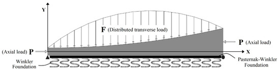
Figure 2.
The geometry of nonuniform nanobeam resting on two linear elastic foundations under axial and transverse loads.
From Equations (10)–(13), the following equation can be derived:
After differentiating Equation (14) twice to x:
From Equations (10) and (15), this equation can be derived:
Equation (16) is a fourth order ordinary differential equation with a variable cross-sectional area of its nanobeam. Subsequently, we provide an overview of the method of its solution (GDQ).
2.2.2. Boundary Conditions
Aiming to cover a wide range of applications, various boundary conditions are used in this article. A simple-simple (SS) supported, a clamped-simple (CS) supported, and a clamped–clamped (CC) supported nanobeams are considered individually in the present research. The following boundary conditions of a nanobeam along the and edges are as follows:
- For the simple-simple supported (SS);
at
at
- For the clamped-simple supported beam (CS);
at
at
- For the clamped–clamped supported nanobeam (CC).
at
at
3. Numerical Mathematical Solution
3.1. Non-Dimensional Analysis
The following non-dimensional terms are applied to transform the governing Equation (16) into a non-dimensional equation.
Then, the non-dimensional form of the governing differential equation is given below:
where
3.2. Solution Methodology (Generalized Differential Quadrature Method Review)
In this task, the DQM [37,51,52,53,54,55,56,57,58] is utilized to subedit the governing differential Equation (23), in a discrete style. The essential feature of the DQM is its ability to approximate the diverse derivatives at a specified point employing a weighted linear sum of functional values at all discrete points in that domain. So, with respect to the DQM, the kth-order derivatives of displacement function at a specified discrete point i in one dimension are determined using the DQ rule [10,56]:
where is the overall number of sampling mesh points in the entire area and are the weighting coefficients. It is known that the weighting coefficients are various at various locations of .
The determination of the weighting coefficient has a vital effect on the accuracy of the results to a greater degree than the formulation of grid points. It took years and huge efforts by scientists to derive more methods to improve the results of applications. Several new branches were birthed from the DQM because of the different methods of determining the weighting coefficient. The method improved by [32], who created the GDQM, was derived and created based on the idea of Bellman’s second approach method [22] with the help of the multiplication approach mentioned in [27]. These formulations present high accuracy and competitiveness in the field of structural systems. From [31], matrix is derived as:
The weighting coefficients of the first derivatives can be obtained from:
for
for
The higher-order weighting coefficients can be easily derived from with the matrix multiplication approach [56], as follows:
From Equations (25)–(29), the precision solution of the DQM is influenced by the selection of the number of spatial grid points, N. The beam is divided into several separate non-equal intervals along the beam in the x-direction. Different assumptions of the grid points have been assumed and tested in this field. Some of them are Legendre-sampling grid points, Radau-sampling grid points, Chebyshev-sampling grid points, Chebyshev–Gauss–Lobatto sampling grid points, and equally spaced-sampling grid points mentioned in detail in [59]. The Chebyshev–Gauss–Lobatto sampling grid points demonstrated high accuracy with equations like our example, so it is used here. From [31], the formulation of the Chebyshev–Gauss–Lobatto sampling grid points is as follows:
The distances among the points are not equal, but these points are condensed at both ends and are quite spaced in the middle.
3.2.1. The Governing Equation
The GDQ method stated above will be utilized to convert the governing Equation (23) into a system of algebraic equations that accordingly follow
where is the value of the function at the grid , and , and are the weighting coefficient matrix of the second, third, and fourth-order derivatives.
3.2.2. Implementation of Boundary Conditions
Some of the boundary conditions can be immediately implemented by employing the substitutions of the boundary conditions into the governing equations (SBCGE) technique. The idea behind the SBCGE method is that the Dirichlet term is carried out at the border points, whilst the derivative term is handled using the GDQ technique; for more details on the SBCGE technique, see references [37,57,58].
Simple-Simple Supported (SS)
For the simple-simple supported nanobeam, the boundary conditions given by the two Equations (17) and (18) can be discretized by the GDQ technique. The given boundary conditions can be written as:
Equations (32) and (34) can be readily replaced in the governing equation, whilst combining the two Equations (33) and (35) yields the following equations
where
Clamped-Simple Supported (CS)
By the same method used in the previous case, the boundary conditions given by the two Equations (19) and (20) can be discretized by the GDQ technique. The given boundary conditions can be written as:
In addition, as in the previous case, Equations (38) and (40) can be readily replaced in the governing equation, while combining the two Equations (39) and (41) yields the following equations
where
Clamped–Clamped Supported (C–S)
Finally, by the same method used in the two previous cases, the boundary conditions given by the two Equations (21) and (22) can be discretized by the GDQ technique. The given boundary conditions can be written as:
Additionally, Equations (44) and (46) can be readily replaced in the governing equation, while combining the two Equations (45) and (47) yields the following equations
where .
Depending on the type of boundary conditions, Equations (36) and (37), Equations (42) and (43), or Equations (48) and (49) for and will be readily replaced in the governing Equation (31) for the interior points . To lock the system, the detached governing Equation (31) must be used at grid points. The dimensions of the equation system utilizing this path are .
It is well known that the Governing Equation (50) has equations for unknowns, which will be set up in matrix shape accordingly.
In all of the examples, a tapered nano wire is subjected to sinusoidally mechanical loading, defined as follows
where is a constant parameter.
4. Numerical Results and Discussion
In this paper, the term describes the deflection in Equation (50) and is calculated by our constructed numerical codes on MATLAB software. The midpoint deflection is studied under the effect of the distributed transverse loads, axial load, double linear elastic foundations, variable cross-sectional area, and the nano-size of the beam. In addition, the midpoint deflection has been reported for different types of boundary conditions, viz., Simple-Simple Supported (SS), Clamped-Simple Supported (CS), and Clamped–Clamped (CC) beams. The different parameters needed for these calculations are as follows:
4.1. Technique Validations
The midpoint deflection for a uniform nanobeam under a distributed load without resting on any elastic foundation or axial forces is compared with the exact analytical results [60]. The results are clarified in Table 1 for simple-simple supported beam (SS) and in Table 2 for the clamped-simple supported beam (CS). Nonuniform grid points () are used in Table 1 and Table 2. The relative error calculated in Table 1 and Table 2 is defined as follows:

Table 1.
Comparison of the middle section deflection for (SS) supported beam with various scaling parameters between the present numerical results and the integral results obtained by Tuna and Kirca.
Table 2.
Comparison of the middle section deflection for (CS) supported beam with various scaling parameters between the present differential numerical results and the integral results by Tuna and Kirca.
The high accuracy of the GDQM is observed by comparing the calculated results with the Laplace Transform (LT) method solution [60] of the simple-simple supported beam, shown in Table 1. The calculated results of Table 1 are illustrated graphically in Figure 3 for the midsection deflection of the nanobeam. The calculated results are in close agreement with the model predictions. One may observe that a close agreement of the calculated results is achieved. However, Table 2 demonstrates the clamped-simple supported nanobeam and gives an 18% error, which is very high! This is the displacement obtained using both integral and differential nonlocal Eringen models. We used the differential model, but [60] used the integral model. These models are identical in symmetric supports such as fixed–fixed supports and simple–simple supports, but they differ in asymmetrical supports such as cantilevers and fixed–simple supports. This paradox is well explained and proved in [61]. By examining Figure 3 and Figure 4 in our present work and comparing them with the same cases in [61] and comparing them with, it is evident that there is a perfect match between the figures, which proves the correctness of our solution.
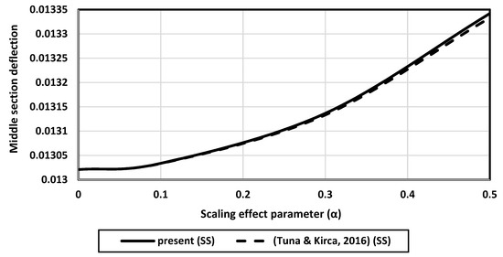
Figure 3.
Comparison between the present numerical results and the exact analytical results [60] for simple-simple supported beam.
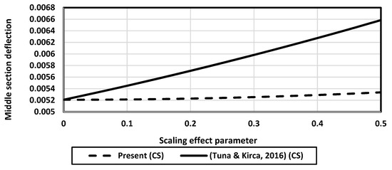
Figure 4.
Comparison between the present numerical results and the exact analytical results [60] for clamped-simple supported beam.
4.2. Results and Discussion
In this section, our calculation results are provided for the mid-section deflection of the possible different cases for a symmetrical and asymmetrical nanobeam under the influence of an axial force and a transverse distributed force , resting on a two-layered elastic foundation and Winkler and Pasternak elastic foundations, under three types of boundary condition- (SS, CS, and CC) supported beams. The effect of the different geometric properties of the nanobeam is given according to the polynomial of by taking two general cases of the varying cross-sectional area of the nanobeam: the first case is that the cross-sectional area changes linearly; the second case is that the cross-sectional area changes parabolically.
The first case entails that the cross-sectional area of the nanobeam changes linearly according to the polynomial , where and are the steepness of the linear polynomial. In this case, we examined the leverage of the steepness of the linear polynomial on the mid-section deflection of the nanobeam by taking four specific situations of the linear nonuniformity distributions according to the steepness of the linear polynomial: the first situation , i.e., ; the second situation , i.e., ; the third situation , i.e., ; and the fourth situation , i.e., the uniform beam , as shown in Figure 5.
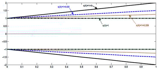
Figure 5.
Different symmetrical and asymmetrical nanobeams change linearly according to the polynomial .
The non-dimensional coefficient of the Winkler elastic foundation , the non-dimensional coefficient of the Pasternak elastic foundation , the non-dimensional distributed force , and the non-dimensional axial force are added one by one for beams with different values of the scaling effect parameter in the next subsections to show how every parameter affects the midpoint deflection and the final results after adding all of them together, under three sets of boundary conditions, shown in Table 3, Table 4, Table 5, Table 6, Table 7, Table 8, Table 9, Table 10, Table 11, Table 12, Table 13 and Table 14.
To provide quick conclusions from Table 3, Table 4, Table 5, Table 6, Table 7, Table 8, Table 9, Table 10, Table 11, Table 12, Table 13 and Table 14, the following can be noted. First, the nondimensional midpoint deflection of the non-uniform nanobeam decreases in comparison with the uniform nanobeam. Second, the steepness of the linear polynomial has a devastating effect on nondimensional midpoint deflection, i.e., the nondimensional midpoint deflection of the non-uniform nanobeam decreases with the increasing steepness of the linear polynomial. Third, the nondimensional midpoint deflection of the nanobeam decreases in the presence of a Winkler elastic foundation under the beam. This decrease in deflection increases by adding the Pasternak elastic foundation under the beam. Fourth, the nondimensional midpoint deflection of the nanobeam increases in the presence of the axial compressive force. Fifth, in the case where the beam is not resting on any foundations, the midpoint deflection of the nanobeam increases with the increasing scaling effect parameter . Conversely, when the beam is resting on a Winkler elastic foundation, the midpoint deflection of the beam decreases with the increasing scaling effect parameter . In addition, when the Pasternak elastic foundation is added under the beam, the midpoint deflection is further decreased with the increase in the scaling effect parameter .
- Simple-Simple supported:
Table 3.
The midpoint deflection for the non-uniform nanobeam with various scaling parameters and the nonuniformity distribution .
Table 3.
The midpoint deflection for the non-uniform nanobeam with various scaling parameters and the nonuniformity distribution .
| Scaling Effect Parameters () | Middle Section Deflection | |||||||||||||||
|---|---|---|---|---|---|---|---|---|---|---|---|---|---|---|---|---|
| 1 | 0 | 0 | 0 | 1 | 30 | 0 | 0 | 1 | 30 | 30 | 0 | 1 | 30 | 30 | 1 | |
| 0 | 0.0088005 | 0.0072758 | 0.0026753 | 0.0027331 | ||||||||||||
| 0.1 | 0.0088092 | 0.0071602 | 0.0025083 | 0.0025639 | ||||||||||||
| 0.2 | 0.0088352 | 0.0068357 | 0.0021133 | 0.0021631 | ||||||||||||
| 0.3 | 0.0088787 | 0.0063590 | 0.0016762 | 0.0017183 | ||||||||||||
| 0.4 | 0.0089395 | 0.0057992 | 0.0013031 | 0.0013376 | ||||||||||||
| 0.5 | 0.0090176 | 0.0052174 | 0.0010166 | 0.0010446 | ||||||||||||
Table 4.
The midpoint deflection for the non-uniform nanobeam with various scaling parameters and the nonuniformity distribution .
Table 4.
The midpoint deflection for the non-uniform nanobeam with various scaling parameters and the nonuniformity distribution .
| Scaling Effect Parameters () | Middle Section Deflection | |||||||||||||||
|---|---|---|---|---|---|---|---|---|---|---|---|---|---|---|---|---|
| 1 | 0 | 0 | 0 | 1 | 30 | 0 | 0 | 1 | 30 | 30 | 0 | 1 | 30 | 30 | 1 | |
| 0 | 0.0104673 | 0.0083809 | 0.0028135 | 0.0028775 | ||||||||||||
| 0.1 | 0.0104776 | 0.0082272 | 0.0026301 | 0.0026913 | ||||||||||||
| 0.2 | 0.0105086 | 0.0077995 | 0.0021998 | 0.0022538 | ||||||||||||
| 0.3 | 0.0105603 | 0.0071818 | 0.0017304 | 0.0017753 | ||||||||||||
| 0.4 | 0.0106326 | 0.0064721 | 0.0013356 | 0.0013719 | ||||||||||||
| 0.5 | 0.0107256 | 0.0057518 | 0.0010362 | 0.0010653 | ||||||||||||
Table 5.
The midpoint deflection for the non-uniform nanobeam with various scaling parameters and the nonuniformity distribution .
Table 5.
The midpoint deflection for the non-uniform nanobeam with various scaling parameters and the nonuniformity distribution .
| Scaling Effect Parameters () | Middle Section Deflection | |||||||||||||||
|---|---|---|---|---|---|---|---|---|---|---|---|---|---|---|---|---|
| 1 | 0 | 0 | 0 | 1 | 30 | 0 | 0 | 1 | 30 | 30 | 0 | 1 | 30 | 30 | 1 | |
| 0 | 0.0115913 | 0.0090872 | 0.0028891 | 0.0029566 | ||||||||||||
| 0.1 | 0.0116027 | 0.0089062 | 0.0026964 | 0.0027607 | ||||||||||||
| 0.2 | 0.0116370 | 0.0084056 | 0.0022463 | 0.0023026 | ||||||||||||
| 0.3 | 0.0116942 | 0.0076904 | 0.0017591 | 0.0018055 | ||||||||||||
| 0.4 | 0.0117743 | 0.0068797 | 0.0013525 | 0.0013897 | ||||||||||||
| 0.5 | 0.0118773 | 0.0060690 | 0.0010463 | 0.0010759 | ||||||||||||
Table 6.
The midpoint deflection for the uniform nanobeam , with various scaling parameters .
Table 6.
The midpoint deflection for the uniform nanobeam , with various scaling parameters .
| Scaling Effect Parameters () | Middle Section Deflection | |||||||||||||||
|---|---|---|---|---|---|---|---|---|---|---|---|---|---|---|---|---|
| 1 | 0 | 0 | 0 | 1 | 30 | 0 | 0 | 1 | 30 | 30 | 0 | 1 | 30 | 30 | 1 | |
| 0 | 0.0130208 | 0.0099433 | 0.0029695 | 0.0030410 | ||||||||||||
| 0.1 | 0.0130337 | 0.0097261 | 0.0027667 | 0.0028344 | ||||||||||||
| 0.2 | 0.0130722 | 0.0091300 | 0.0022951 | 0.0023539 | ||||||||||||
| 0.3 | 0.0131365 | 0.0082892 | 0.0017888 | 0.0018369 | ||||||||||||
| 0.4 | 0.0132265 | 0.0073516 | 0.0013700 | 0.0014082 | ||||||||||||
| 0.5 | 0.0133421 | 0.0064298 | 0.0010566 | 0.0010869 | ||||||||||||
- Clamped-Simple supported:
Table 7.
The midpoint deflection for the non-uniform nanobeam with various scaling parameters and the nonuniformity distribution .
Table 7.
The midpoint deflection for the non-uniform nanobeam with various scaling parameters and the nonuniformity distribution .
| Scaling Effect Parameters () | Middle Section Deflection | |||||||||||||||
|---|---|---|---|---|---|---|---|---|---|---|---|---|---|---|---|---|
| 1 | 0 | 0 | 0 | 1 | 30 | 0 | 0 | 1 | 30 | 30 | 0 | 1 | 30 | 30 | 1 | |
| 0 | 0.0037978 | 0.0034813 | 0.0018206 | 0.0018498 | ||||||||||||
| 0.1 | 0.0038015 | 0.0034530 | 0.0016346 | 0.0016638 | ||||||||||||
| 0.2 | 0.0038127 | 0.0033711 | 0.0012577 | 0.0012846 | ||||||||||||
| 0.3 | 0.0038315 | 0.0032440 | 0.0009141 | 0.0009365 | ||||||||||||
| 0.4 | 0.0038577 | 0.0030834 | 0.0006645 | 0.0006824 | ||||||||||||
| 0.5 | 0.0038915 | 0.0029018 | 0.0004942 | 0.0005083 | ||||||||||||
Table 8.
The midpoint deflection for the non-uniform nanobeam with various scaling parameters and the nonuniformity distribution .
Table 8.
The midpoint deflection for the non-uniform nanobeam with various scaling parameters and the nonuniformity distribution .
| Scaling Effect Parameters () | Middle Section Deflection | |||||||||||||||
|---|---|---|---|---|---|---|---|---|---|---|---|---|---|---|---|---|
| 1 | 0 | 0 | 0 | 1 | 30 | 0 | 0 | 1 | 30 | 30 | 0 | 1 | 30 | 30 | 1 | |
| 0 | 0.0043704 | 0.0039543 | 0.0019298 | 0.0019630 | ||||||||||||
| 0.1 | 0.0043747 | 0.0039166 | 0.0017247 | 0.0017574 | ||||||||||||
| 0.2 | 0.0043877 | 0.0038082 | 0.0013131 | 0.0013424 | ||||||||||||
| 0.3 | 0.0044092 | 0.0036418 | 0.0009441 | 0.0009680 | ||||||||||||
| 0.4 | 0.0044394 | 0.0034345 | 0.0006806 | 0.0006992 | ||||||||||||
| 0.5 | 0.0044783 | 0.0032042 | 0.0005031 | 0.0005176 | ||||||||||||
Table 9.
The midpoint deflection for the non-uniform nanobeam with various scaling parameters and the nonuniformity distribution .
Table 9.
The midpoint deflection for the non-uniform nanobeam with various scaling parameters and the nonuniformity distribution .
| Scaling Effect Parameters () | Middle Section Deflection | |||||||||||||||
|---|---|---|---|---|---|---|---|---|---|---|---|---|---|---|---|---|
| 1 | 0 | 0 | 0 | 1 | 30 | 0 | 0 | 1 | 30 | 30 | 0 | 1 | 30 | 30 | 1 | |
| 0 | 0.0047446 | 0.0042562 | 0.0019906 | 0.0020261 | ||||||||||||
| 0.1 | 0.0047493 | 0.0042117 | 0.0017745 | 0.0018092 | ||||||||||||
| 0.2 | 0.0047633 | 0.0040842 | 0.0013431 | 0.0013738 | ||||||||||||
| 0.3 | 0.0047867 | 0.0038899 | 0.0009600 | 0.0009847 | ||||||||||||
| 0.4 | 0.0048195 | 0.0036502 | 0.0006889 | 0.0007081 | ||||||||||||
| 0.5 | 0.0048617 | 0.0033869 | 0.0005077 | 0.0005225 | ||||||||||||
Table 10.
The midpoint deflection for the uniform nanobeam , with various scaling parameters .
Table 10.
The midpoint deflection for the uniform nanobeam , with various scaling parameters .
| Scaling Effect Parameters () | Middle Section Deflection | |||||||||||||||
|---|---|---|---|---|---|---|---|---|---|---|---|---|---|---|---|---|
| 1 | 0 | 0 | 0 | 1 | 30 | 0 | 0 | 1 | 30 | 30 | 0 | 1 | 30 | 30 | 1 | |
| 0 | 0.0052083 | 0.0046225 | 0.0020561 | 0.0020943 | ||||||||||||
| 0.1 | 0.0052135 | 0.0045688 | 0.0018279 | 0.0018649 | ||||||||||||
| 0.2 | 0.0052289 | 0.0044158 | 0.0013749 | 0.0014071 | ||||||||||||
| 0.3 | 0.0052546 | 0.0041847 | 0.0009766 | 0.0010022 | ||||||||||||
| 0.4 | 0.0052906 | 0.0039030 | 0.0006976 | 0.0007172 | ||||||||||||
| 0.5 | 0.0053368 | 0.0035977 | 0.0005124 | 0.0005275 | ||||||||||||
- Clamped–Clamped supported:
Table 11.
The midpoint deflection for the non-uniform nanobeam with various scaling parameters and the nonuniformity distribution .
Table 11.
The midpoint deflection for the non-uniform nanobeam with various scaling parameters and the nonuniformity distribution .
| Scaling Effect Parameters () | Middle Section Deflection | |||||||||||||||
|---|---|---|---|---|---|---|---|---|---|---|---|---|---|---|---|---|
| 1 | 0 | 0 | 0 | 1 | 30 | 0 | 0 | 1 | 30 | 30 | 0 | 1 | 30 | 30 | 1 | |
| 0 | 0.0017769 | 0.0017059 | 0.0011447 | 0.0011573 | ||||||||||||
| 0.1 | 0.0017786 | 0.0016992 | 0.0010071 | 0.0010209 | ||||||||||||
| 0.2 | 0.0017839 | 0.0016795 | 0.0007426 | 0.0007566 | ||||||||||||
| 0.3 | 0.0017926 | 0.0016479 | 0.0005187 | 0.0005308 | ||||||||||||
| 0.4 | 0.0018049 | 0.0016061 | 0.0003663 | 0.0003759 | ||||||||||||
| 0.5 | 0.0018207 | 0.0015563 | 0.0002671 | 0.0002746 | ||||||||||||
Table 12.
The midpoint deflection for the non-uniform nanobeam with various scaling parameters and the nonuniformity distribution .
Table 12.
The midpoint deflection for the non-uniform nanobeam with various scaling parameters and the nonuniformity distribution .
| Scaling Effect Parameters () | Middle Section Deflection | |||||||||||||||
|---|---|---|---|---|---|---|---|---|---|---|---|---|---|---|---|---|
| 1 | 0 | 0 | 0 | 1 | 30 | 0 | 0 | 1 | 30 | 30 | 0 | 1 | 30 | 30 | 1 | |
| 0 | 0.0021003 | 0.0020022 | 0.0012722 | 0.0012877 | ||||||||||||
| 0.1 | 0.0021024 | 0.0019926 | 0.0011059 | 0.0011225 | ||||||||||||
| 0.2 | 0.0021086 | 0.0019647 | 0.0007963 | 0.0008123 | ||||||||||||
| 0.3 | 0.0021190 | 0.0019201 | 0.0005447 | 0.0005580 | ||||||||||||
| 0.4 | 0.0021335 | 0.0018618 | 0.0003791 | 0.0003895 | ||||||||||||
| 0.5 | 0.0021521 | 0.0017930 | 0.0002738 | 0.0002818 | ||||||||||||
Table 13.
The midpoint deflection for the non-uniform nanobeam with various scaling parameters and the nonuniformity distribution .
Table 13.
The midpoint deflection for the non-uniform nanobeam with various scaling parameters and the nonuniformity distribution .
| Scaling Effect Parameters () | Middle Section Deflection | |||||||||||||||
|---|---|---|---|---|---|---|---|---|---|---|---|---|---|---|---|---|
| 1 | 0 | 0 | 0 | 1 | 30 | 0 | 0 | 1 | 30 | 30 | 0 | 1 | 30 | 30 | 1 | |
| 0 | 0.0023206 | 0.0022015 | 0.0013504 | 0.0013679 | ||||||||||||
| 0.1 | 0.0023229 | 0.0021897 | 0.0011651 | 0.0011835 | ||||||||||||
| 0.2 | 0.0023297 | 0.0021554 | 0.0008269 | 0.0008442 | ||||||||||||
| 0.3 | 0.0023412 | 0.0021010 | 0.0005589 | 0.0005729 | ||||||||||||
| 0.4 | 0.0023572 | 0.0020302 | 0.0003860 | 0.0003967 | ||||||||||||
| 0.5 | 0.0023778 | 0.0019472 | 0.0002773 | 0.0002855 | ||||||||||||
Table 14.
The midpoint deflection for the uniform nanobeam , with various scaling parameters .
Table 14.
The midpoint deflection for the uniform nanobeam , with various scaling parameters .
| Scaling Effect Parameters () | Middle Section Deflection | |||||||||||||||
|---|---|---|---|---|---|---|---|---|---|---|---|---|---|---|---|---|
| 1 | 0 | 0 | 0 | 1 | 30 | 0 | 0 | 1 | 30 | 30 | 0 | 1 | 30 | 30 | 1 | |
| 0 | 0.0026042 | 0.0024552 | 0.0014421 | 0.0014624 | ||||||||||||
| 0.1 | 0.0026067 | 0.0024403 | 0.0012331 | 0.0012537 | ||||||||||||
| 0.2 | 0.0026144 | 0.0023970 | 0.0008606 | 0.0008794 | ||||||||||||
| 0.3 | 0.0026273 | 0.0023287 | 0.0005741 | 0.0005889 | ||||||||||||
| 0.4 | 0.0026453 | 0.0022405 | 0.0003931 | 0.0004042 | ||||||||||||
| 0.5 | 0.0026684 | 0.0021381 | 0.0002810 | 0.0002894 | ||||||||||||
The second case in this study is that the cross-sectional area of the nanobeam changes parabolically according to the polynomial .
In this case, we examined the leverage of the polynomial equation of a second degree on the deflection of the nanobeam by taking three specific situations of the asymmetricity distributions; the first situation , i.e., ; the second situation , i.e., ; and the third situation , i.e., , as shown in Figure 6.
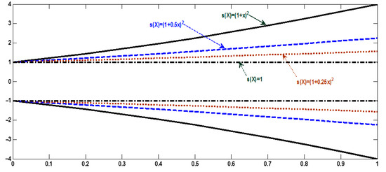
Figure 6.
Different cross-sectional areas of the symmetric and asymmetric nanobeams change parabolically according to the polynomial .
For quick conclusions from Table 15, Table 16, Table 17, Table 18, Table 19, Table 20, Table 21, Table 22 and Table 23, the following can be noted. First, the constant of the polynomial has a devastating effect on nondimensional midpoint deflection, i.e., the nondimensional midpoint deflection of the asymmetric nanobeam decreases with the increasing constant of the polynomial. Second, the nondimensional midpoint deflection of nanobeam decreases in the presence of a Winkler elastic foundation under the beam. This decrease in deflection increases by adding the Pasternak elastic foundation under the beam. Third, the nondimensional midpoint deflection of the nanobeam increases in the presence of an axial compressive force. Fourth, in the case where the beam is not resting on any foundations, the midpoint deflection of the nanobeam increases when increasing the scaling effect parameter ; conversely, when the beam is resting on a Winkler elastic foundation, the midpoint deflection of the beam decreases when increasing the scaling effect parameter . Fifth, when the Pasternak elastic foundation is added under the beam, the midpoint deflection is further decreased with the increase in the scaling effect parameter .
- Simple-Simple supported:
Table 15.
The midpoint deflection for the non-uniform nanobeam with various scaling parameters and the nonuniformity distribution .
Table 15.
The midpoint deflection for the non-uniform nanobeam with various scaling parameters and the nonuniformity distribution .
| Scaling Effect Parameters () | Middle Section Deflection | |||||||||||||||
|---|---|---|---|---|---|---|---|---|---|---|---|---|---|---|---|---|
| 1 | 0 | 0 | 0 | 1 | 30 | 0 | 0 | 1 | 30 | 30 | 0 | 1 | 30 | 30 | 1 | |
| 0 | 0.0060328 | 0.0052717 | 0.0023373 | 0.0023814 | ||||||||||||
| 0.1 | 0.0060387 | 0.0052114 | 0.0022065 | 0.0022496 | ||||||||||||
| 0.2 | 0.0060566 | 0.0050391 | 0.0018915 | 0.0019315 | ||||||||||||
| 0.3 | 0.0060863 | 0.0047780 | 0.0015317 | 0.0015670 | ||||||||||||
| 0.4 | 0.0061280 | 0.0044584 | 0.0012135 | 0.0012434 | ||||||||||||
| 0.5 | 0.0061816 | 0.0041105 | 0.0009611 | 0.0009862 | ||||||||||||
Table 16.
The midpoint deflection for the non-uniform nanobeam with various scaling parameters and the nonuniformity distribution .
Table 16.
The midpoint deflection for the non-uniform nanobeam with various scaling parameters and the nonuniformity distribution .
| Scaling Effect Parameters () | Middle Section Deflection | |||||||||||||||
|---|---|---|---|---|---|---|---|---|---|---|---|---|---|---|---|---|
| 1 | 0 | 0 | 0 | 1 | 30 | 0 | 0 | 1 | 30 | 30 | 0 | 1 | 30 | 30 | 1 | |
| 0 | 0.0084559 | 0.0070382 | 0.0026414 | 0.0026977 | ||||||||||||
| 0.1 | 0.0084642 | 0.0069300 | 0.0024781 | 0.0025324 | ||||||||||||
| 0.2 | 0.0084893 | 0.0066258 | 0.0020914 | 0.0021401 | ||||||||||||
| 0.3 | 0.0085310 | 0.0061773 | 0.0016621 | 0.0017036 | ||||||||||||
| 0.4 | 0.0085894 | 0.0056481 | 0.0012945 | 0.0013286 | ||||||||||||
| 0.5 | 0.0086645 | 0.0050953 | 0.0010114 | 0.0010391 | ||||||||||||
Table 17.
The midpoint deflection for the non-uniform nanobeam with various scaling parameters and the nonuniformity distribution .
Table 17.
The midpoint deflection for the non-uniform nanobeam with various scaling parameters and the nonuniformity distribution .
| Scaling Effect Parameters () | Middle Section Deflection | |||||||||||||||
|---|---|---|---|---|---|---|---|---|---|---|---|---|---|---|---|---|
| 1 | 0 | 0 | 0 | 1 | 30 | 0 | 0 | 1 | 30 | 30 | 0 | 1 | 30 | 30 | 1 | |
| 0 | 0.0103341 | 0.0082953 | 0.0028038 | 0.0028673 | ||||||||||||
| 0.1 | 0.0103443 | 0.0081447 | 0.0026215 | 0.0026822 | ||||||||||||
| 0.2 | 0.0103749 | 0.0077254 | 0.0021937 | 0.0022473 | ||||||||||||
| 0.3 | 0.0104259 | 0.0071192 | 0.0017266 | 0.0017713 | ||||||||||||
| 0.4 | 0.0104973 | 0.0064214 | 0.0013333 | 0.0013694 | ||||||||||||
| 0.5 | 0.0105891 | 0.0057121 | 0.0010348 | 0.0010638 | ||||||||||||
- Clamped-Simple supported:
Table 18.
The midpoint deflection for the non-uniform nanobeam with various scaling parameters and the nonuniformity distribution .
Table 18.
The midpoint deflection for the non-uniform nanobeam with various scaling parameters and the nonuniformity distribution .
| Scaling Effect Parameters () | Middle Section Deflection | |||||||||||||||
|---|---|---|---|---|---|---|---|---|---|---|---|---|---|---|---|---|
| 1 | 0 | 0 | 0 | 1 | 30 | 0 | 0 | 1 | 30 | 30 | 0 | 1 | 30 | 30 | 1 | |
| 0 | 0.0027714 | 0.0026007 | 0.0015625 | 0.0015835 | ||||||||||||
| 0.1 | 0.0027741 | 0.0025860 | 0.0014172 | 0.0014389 | ||||||||||||
| 0.2 | 0.0027824 | 0.0025432 | 0.0011174 | 0.0011386 | ||||||||||||
| 0.3 | 0.0027960 | 0.0024755 | 0.0008340 | 0.0008527 | ||||||||||||
| 0.4 | 0.0028152 | 0.0023875 | 0.0006199 | 0.0006354 | ||||||||||||
| 0.5 | 0.0028398 | 0.0022848 | 0.0004687 | 0.0004813 | ||||||||||||
Table 19.
The midpoint deflection for the non-uniform nanobeam with various scaling parameters and the nonuniformity distribution .
Table 19.
The midpoint deflection for the non-uniform nanobeam with various scaling parameters and the nonuniformity distribution .
| Scaling Effect Parameters () | Middle Section Deflection | |||||||||||||||
|---|---|---|---|---|---|---|---|---|---|---|---|---|---|---|---|---|
| 1 | 0 | 0 | 0 | 1 | 30 | 0 | 0 | 1 | 30 | 30 | 0 | 1 | 30 | 30 | 1 | |
| 0 | 0.0036685 | 0.0033731 | 0.0017939 | 0.0018222 | ||||||||||||
| 0.1 | 0.0036721 | 0.0033467 | 0.0016122 | 0.0016405 | ||||||||||||
| 0.2 | 0.0036830 | 0.0032705 | 0.0012433 | 0.0012696 | ||||||||||||
| 0.3 | 0.0037011 | 0.0031518 | 0.0009060 | 0.0009280 | ||||||||||||
| 0.4 | 0.0037264 | 0.0030013 | 0.0006601 | 0.0006777 | ||||||||||||
| 0.5 | 0.0037590 | 0.0028305 | 0.0004917 | 0.0005056 | ||||||||||||
Table 20.
The midpoint deflection for the non-uniform nanobeam with various scaling parameters and the nonuniformity distribution .
Table 20.
The midpoint deflection for the non-uniform nanobeam with various scaling parameters and the nonuniformity distribution .
| Scaling Effect Parameters () | Middle Section Deflection | |||||||||||||||
|---|---|---|---|---|---|---|---|---|---|---|---|---|---|---|---|---|
| 1 | 0 | 0 | 0 | 1 | 30 | 0 | 0 | 1 | 30 | 30 | 0 | 1 | 30 | 30 | 1 | |
| 0 | 0.0043226 | 0.0039155 | 0.0019220 | 0.0019548 | ||||||||||||
| 0.1 | 0.0043269 | 0.0038787 | 0.0017182 | 0.0017506 | ||||||||||||
| 0.2 | 0.0043397 | 0.0037727 | 0.0013090 | 0.0013381 | ||||||||||||
| 0.3 | 0.0043610 | 0.0036097 | 0.0009418 | 0.0009656 | ||||||||||||
| 0.4 | 0.0043909 | 0.0034066 | 0.0006794 | 0.0006980 | ||||||||||||
| 0.5 | 0.0044293 | 0.0031806 | 0.0005025 | 0.0005169 | ||||||||||||
- Clamped–Clamped supported:
Table 21.
The midpoint deflection for the non-uniform nanobeam with various scaling parameters and the nonuniformity distribution .
Table 21.
The midpoint deflection for the non-uniform nanobeam with various scaling parameters and the nonuniformity distribution .
| Scaling Effect Parameters () | Middle Section Deflection | |||||||||||||||
|---|---|---|---|---|---|---|---|---|---|---|---|---|---|---|---|---|
| 1 | 0 | 0 | 0 | 1 | 30 | 0 | 0 | 1 | 30 | 30 | 0 | 1 | 30 | 30 | 1 | |
| 0 | 0.0012030 | 0.0011696 | 0.0008711 | 0.0008785 | ||||||||||||
| 0.1 | 0.0012042 | 0.0011667 | 0.0007851 | 0.0007936 | ||||||||||||
| 0.2 | 0.0012077 | 0.0011582 | 0.0006100 | 0.0006196 | ||||||||||||
| 0.3 | 0.0012137 | 0.0011445 | 0.0004484 | 0.0004575 | ||||||||||||
| 0.4 | 0.0012220 | 0.0011260 | 0.0003291 | 0.0003370 | ||||||||||||
| 0.5 | 0.0012327 | 0.0011034 | 0.0002466 | 0.0002531 | ||||||||||||
Table 22.
The midpoint deflection for the non-uniform nanobeam with various scaling parameters and the nonuniformity distribution .
Table 22.
The midpoint deflection for the non-uniform nanobeam with various scaling parameters and the nonuniformity distribution .
| Scaling Effect Parameters () | Middle Section Deflection | |||||||||||||||
|---|---|---|---|---|---|---|---|---|---|---|---|---|---|---|---|---|
| 1 | 0 | 0 | 0 | 1 | 30 | 0 | 0 | 1 | 30 | 30 | 0 | 1 | 30 | 30 | 1 | |
| 0 | 0.0016894 | 0.0016250 | 0.0011062 | 0.0011181 | ||||||||||||
| 0.1 | 0.0016910 | 0.0016190 | 0.0009766 | 0.0009896 | ||||||||||||
| 0.2 | 0.0016960 | 0.0016012 | 0.0007253 | 0.0007387 | ||||||||||||
| 0.3 | 0.0017044 | 0.0015726 | 0.0005100 | 0.0005217 | ||||||||||||
| 0.4 | 0.0017161 | 0.0015348 | 0.0003619 | 0.0003713 | ||||||||||||
| 0.5 | 0.0017311 | 0.0014895 | 0.0002647 | 0.0002721 | ||||||||||||
Table 23.
The midpoint deflection for the non-uniform nanobeam with various scaling parameters and the nonuniformity distribution .
Table 23.
The midpoint deflection for the non-uniform nanobeam with various scaling parameters and the nonuniformity distribution .
| Scaling Effect Parameters () | Middle Section Deflection | |||||||||||||||
|---|---|---|---|---|---|---|---|---|---|---|---|---|---|---|---|---|
| 1 | 0 | 0 | 0 | 1 | 30 | 0 | 0 | 1 | 30 | 30 | 0 | 1 | 30 | 30 | 1 | |
| 0 | 0.0020661 | 0.0019711 | 0.0012590 | 0.0012743 | ||||||||||||
| 0.1 | 0.0020682 | 0.0019618 | 0.0010959 | 0.0011122 | ||||||||||||
| 0.2 | 0.0020743 | 0.0019348 | 0.0007910 | 0.0008068 | ||||||||||||
| 0.3 | 0.0020845 | 0.0018916 | 0.0005422 | 0.0005554 | ||||||||||||
| 0.4 | 0.0020988 | 0.0018351 | 0.0003779 | 0.0003882 | ||||||||||||
| 0.5 | 0.0021171 | 0.0017683 | 0.0002732 | 0.0002811 | ||||||||||||
The following Figure 7, Figure 8, Figure 9, Figure 10, Figure 11 and Figure 12 show the influence of the varying cross-sectional area of the nanobeam, with three different types of supports (Figure 7, Figure 8 and Figure 9 for the first case of the inertia ratio and Figure 10, Figure 11 and Figure 12 for the second case of the inertia ratio).
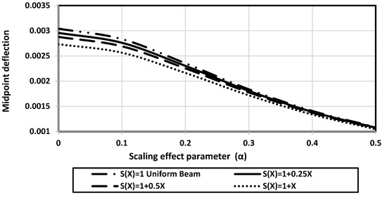
Figure 7.
The influence of the varying cross-sectional area of the simple-simple supported nanobeam linearly according to the polynomial on the midpoint deflection.
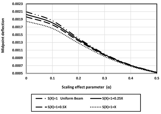
Figure 8.
The influence of the varying cross-sectional area of the clamped-simple supported nanobeam linearly according to the polynomial on the midpoint deflection.
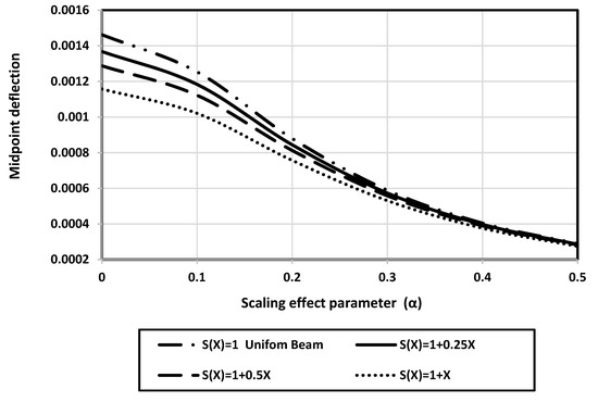
Figure 9.
The influence of the varying cross-sectional area of the clamped–clamped nanobeam linearly according to the polynomial on the midpoint deflection.
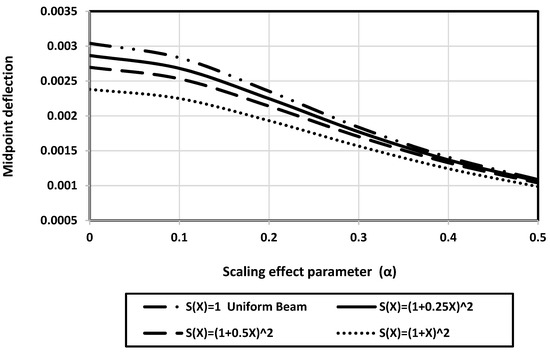
Figure 10.
The influence of the varying cross-sectional area of the simple-simple supported nanobeam parabolically according to the polynomial on the midpoint deflection.
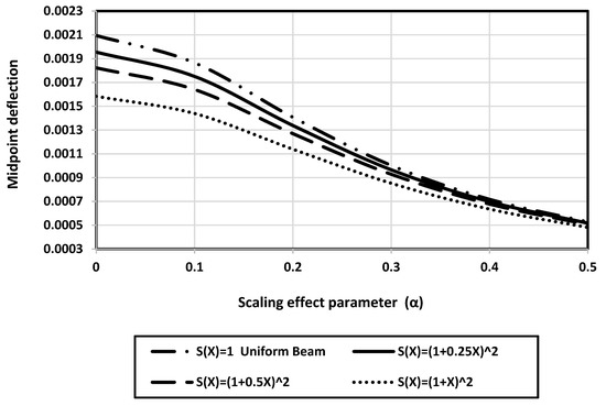
Figure 11.
The influence of the varying cross-sectional area of the clamped-simple supported nanobeam parabolically according to the polynomial on the midpoint deflection.
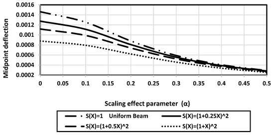
Figure 12.
The influence of the varying cross-sectional area of the clamped–clamped supported nanobeam parabolically according to the polynomial on the midpoint deflection.
The general form of the beam equation is ; this means that the values of and control the deflection of the beam.
Table 24 and Table 25, show the effect of the values of and on the deflection of the nonuniform nanobeam, whose cross-sectional area changes linearly and parabolically for the three sets of boundary conditions. It is assumed for the nanobeam that, at foundation parameters , the non-dimensional distributed force , the non-dimensional axial force , and the scaling effect parameter .
Table 24.
The effect of the nonuniformity parameter of the nanobeam changed linearly according to the polynomial on the midpoint deflection.
Table 25.
The effect of the nonuniformity parameters and of the nanobeam changed parabolically according to the polynomial on the midpoint deflection.
Table 24 describes the first case, where the cross-sectional area of the nanobeam changes linearly according to the polynomial , where . This means that, in this case, we are studying the influence of changing the nonuniformity parameter on the deflection of the beam. In addition, Table 24 presents a comparison of the deflection of the beam between the uniform and nonuniform changes linearly for the three sets of boundary conditions.
Table 25 describes the second case, where the cross-sectional area of the nanobeam changes parabolically according to the polynomial . This means that we are studying the effect of changing the nonuniformity parameters and on the deflection of the beam. In addition, Table 25 presents a comparison of the deflection of the nonuniform beam changes linearly and parabolically, for the three sets of boundary conditions.
Table 24 and Table 25 briefly show the effect of changing the nonuniformity parameters and of the nanobeam on midpoint deflection.
From Table 24 and Table 25, the midpoint deflection decreases with the increase in or the increase in .
Figure 12, Figure 13 and Figure 14 present a comparison between the uniform and nonuniform parameters (whose cross-sectional area changes linearly and parabolically) of the nanobeam on the midpoint deflection for the three sets of boundary conditions.
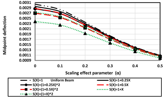
Figure 13.
The effect of the nonuniformity parameters and of simple-simple supported nanobeam according to the polynomial on the midpoint deflection.
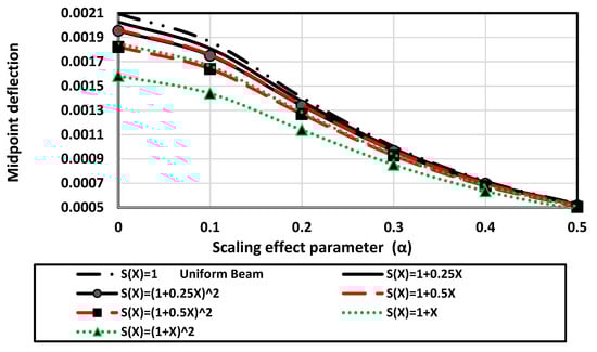
Figure 14.
The effect of the nonuniformity parameters and of clamped-simple supported nanobeam according to the polynomial on the midpoint deflection.
From Figure 13, Figure 14 and Figure 15, the following can be noted. First, the midpoint deflection of the non-uniform nanobeam decreases in comparison with the uniform nanobeam. Second, the midpoint deflection decreases with the increase in or the increase in .
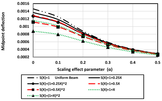
Figure 15.
The effect of the nonuniformity parameters and of clamped–clamped-supported nanobeam according to the polynomial on the midpoint deflection.
5. Conclusions
The high accuracy of the GDQM can be observed by comparing the calculated results with the analytical solution [60]. This article focused on investigating the effects of many different parameters. The first investigation (the main investigation) studied the effect of the nonlocal (scaling effect) parameter on the deflection of uniform and nonuniform nanobeams, whose cross-sectional area changes linearly and parabolically, in accordance with a polynomial of the form , resting on two types of linear elastic foundations, and under three sets of boundary conditions. The second investigation studied the effect of nonuniformity (the varying cross-sectional area) on the deflection of the nanobeam, in accordance with the polynomial of the form , for various values of the scaling effect parameter, and under three sets of boundary conditions. Finally, the third investigation studied the effect of the presence of two linear elastic foundations (the Winkler elastic foundation and Pasternak elastic foundation) on the deflection of a nanobeam whose cross-sectional area changes linearly and parabolically, in accordance with a polynomial of the form , for various values of scaling effect parameters and under the three sets of boundary conditions.
The number of influencing factors used yielded many cases that can be studied and analyzed according to these influences, which need pages and pages of study, analysis, and comparisons. For all these results, as well as the relationships that exist between the influencing factors used in the research, their maximum and minimum values can be deduced through the process of optimization according to the type of application in which these variables will be used.
Regarding the use of the suggested technicality of the GDQM to evaluate the nondimensional deflection of the nanobeam, this study’s quick conclusions can be summarized as follows:
- The nondimensional deflection of the nonuniform nanobeam decreases in comparison with the uniform nanobeam.
- It was found that the nondimensional deflection of the nanobeam is reduced with the decrease in the scaling effect parameter of the nanobeams.
- When the nanobeam is not resting on any elastic foundations, the nondimensional deflection increases when increasing the scaling effect parameter. Conversely, when the nanobeam is resting on an elastic foundation, the nondimensional deflection of the nanobeam decreases when increasing the scaling effect parameter.
- When the cross-sectional area of the nanobeam varies linearly, the nondimensional deflection of the nanobeam decreases when increasing the steepness of the linear polynomial.
- When the cross-sectional area of the nanobeam varies parabolically, the non-dimensional deflection of the non-uniform nanobeam decreases compared to when the cross-sectional area varies linearly.
- When the nanobeam is resting on an elastic foundation, the nondimensional deflection of the nanobeam decreases.
- The minimum degree of nondimensional deflection can be found from a clamped–clamped-supported beam, followed by the clamped-simple supported beam, while the maximum degree of nondimensional deflection can be found from a simple-simple supported beam.
For future work, this paper can provide several directions regarding research and applications. For example:
- It can be converted into a computer program that calculates the deflection of any point in beams with any cross sections resting on linear foundations. Different types of linear and non-linear foundations and surrounding mediums can also be added to widen the applications used.
- A dynamic study of the same applications can be undertaken to intitiate a series of static and dynamic studies that covers beams, plates, shells, connecting rods, and nanosystems to improve the field of nanomachines and nanorobots.
Author Contributions
Conceptualization. I.M.E. and R.M.A.; methodology, M.H.K. and H.A.; software, A.L.F.; validation, I.M.E., M.A.E.-S. and R.M.A.; formal analysis, I.M.E. and H.A.; investigation, R.M.A.; resources, M.H.K.; data curation, A.L.F.; writing—original draft preparation, I.M.E., M.A.E.-S. and R.M.A.; writing—review and editing, I.M.E., H.A. and R.M.A.; visualization, M.A.E.-S.; supervision, I.M.E.; project administration, M.H.K.; funding acquisition, H.A. All authors have read and agreed to the published version of the manuscript.
Funding
This research received no external funding.
Data Availability Statement
Not applicable.
Acknowledgments
We are very thankful for the reviewer’s excellent suggestions, which have greatly improved the quality of our paper. The work of H. Alotaibi is supported by Taif University Researchers Supporting Project Number (TURSP-2020/304), Taif University, Taif, Saudi Arabia.
Conflicts of Interest
The authors declare no conflict of interest.
References
- Iijima, S. Helical microtubules of graphitic carbon. Nature 1991, 354, 56–58. [Google Scholar] [CrossRef]
- Wang, X.; Bert, C.W.; Striz, A.G. Differential quadrature analysis of deflection, buckling, and free vibration of beams and rectangular plates. Comput. Struct. 1993, 48, 473–479. [Google Scholar] [CrossRef]
- Chen, W.; Striz, A.G.; Bert, C.W. A new approach to the differential quadrature method for fourth-order equations. Int. J. Numer. Methods Eng. 1997, 40, 1941–1956. [Google Scholar] [CrossRef]
- Civalek, Ö.; Demir, Ç. Bending analysis of microtubules using nonlocal Euler-Bernoulli beam theory. Appl. Math. Model. 2011, 35, 2053–2067. [Google Scholar] [CrossRef]
- Hosseini-Hashemi, S.; Fakher, M.; Nazemnezhad, R. Surface effects on free vibration analysis of nanobeams using nonlocal elasticity: A comparison between Euler-Bernoulli and Timoshenko. J. Solid Mech. 2013, 15, 290–304. [Google Scholar]
- Jena, S.K.; Chakraverty, S. Differential quadrature and differential transformation methods in buckling analysis of nanobeams. Curved Layer. Struct. 2019, 6, 68–76. [Google Scholar] [CrossRef]
- Zhong, H.; Guo, Q. Nonlinear vibration analysis of Timoshenko beams using the differential quadrature method. Nonlinear Dyn. 2003, 32, 223–234. [Google Scholar] [CrossRef]
- Emam, S.A. A general nonlocal nonlinear model for buckling of nanobeams. Appl. Math. Model. 2013, 37, 6929–6939. [Google Scholar] [CrossRef]
- Karami, B.; Janghorban, M.; Dimitri, R.; Tornabene, F. Free vibration analysis of triclinic nanobeams based on the differential quadrature method. Appl. Sci. 2019, 9, 3517. [Google Scholar] [CrossRef]
- Behera, L.; Chakraverty, S. Application of Differential Quadrature method in free vibration analysis of nanobeams based on various nonlocal theories. Comput. Math. Appl. 2015, 69, 1444–1462. [Google Scholar] [CrossRef]
- Baughman, R.H.; Zakhidov, A.A.; de Heer, W.A. Carbon nanotubes-the route toward applications. Science 2002, 297, 787–792. [Google Scholar] [CrossRef] [PubMed]
- Eringen, A.C. On differential equations of nonlocal elasticity and solutions of screw dislocation and surface waves. J. Appl. Phys. 1983, 54, 4703–4710. [Google Scholar] [CrossRef]
- Eringen, A.C. Nonlocal continuum mechanics based on distributions. Int. J. Eng. Sci. 2006, 44, 141–147. [Google Scholar] [CrossRef]
- Kerr, A.D. Elastic and Viscoelastic Foundation Models; ASME: New York, NY, USA, 1964. [Google Scholar]
- Zhang, R.; Bai, H.; Chen, X. The Consistent Couple Stress Theory-Based Vibration and Post-Buckling Analysis of Bi-directional Functionally Graded Microbeam. Symmetry 2022, 14, 602. [Google Scholar] [CrossRef]
- Chaluvaraju, B.V.; Afzal, A.; Vinnik, D.A.; Kaladgi, A.R.; Alamri, S.; Tirth, V. Mechanical and corrosion studies of friction stir welded nano Al2O3 reinforced Al-Mg matrix composites: RSM-ANN modelling approach. Symmetry 2021, 13, 537. [Google Scholar]
- Abouelregal, A.E.; Marin, M. The response of nanobeams with temperature-dependent properties using state-space method via modified couple stress theory. Symmetry 2020, 12, 1276. [Google Scholar] [CrossRef]
- Malikan, M.; Eremeyev, V.A.; Żur, K.K. Effect of axial porosities on flexomagnetic response of in-plane compressed piezomagnetic nanobeams. Symmetry 2020, 12, 1935. [Google Scholar] [CrossRef]
- Malikan, M.; Eremeyev, V.A. On the dynamics of a visco–piezo–flexoelectric nanobeam. Symmetry 2020, 12, 643. [Google Scholar] [CrossRef]
- Barretta, R.; Čanađija, M.; de Sciarra, F.M. Nonlocal mechanical behavior of layered nanobeams. Symmetry 2020, 12, 717. [Google Scholar] [CrossRef]
- Bellman, R.; Casti, J. Differential quadrature and long-term integration. J. Math. Anal. Appl. 1971, 34, 235–238. [Google Scholar] [CrossRef]
- Bellman, R.; Kashef, B.G.; Casti, J. Differential quadrature: A technique for the rapid solution of nonlinear partial differential equations. J. Comput. Phys. 1972, 10, 40–52. [Google Scholar] [CrossRef]
- Mingle, J.O. Computational considerations in non-linear diffusion. Int. J. Numer. Methods Eng. 1973, 7, 103–116. [Google Scholar] [CrossRef]
- Mingle, J.O. The method of differential quadrature for transient nonlinear diffusion. J. Math. Anal. Appl. 1977, 60, 559–569. [Google Scholar] [CrossRef][Green Version]
- Civan, F.; Sliepcevich, C.M. Application of differential quadrature to transport processes. J. Math. Anal. Appl. 1983, 93, 206–221. [Google Scholar] [CrossRef][Green Version]
- Civan, F.; Sliepcevich, C.M. Solution of the Poisson equation by differential quadrature. Int. J. Numer. Methods Eng. 1983, 19, 711–724. [Google Scholar] [CrossRef]
- Civan, F.; Sliepcevich, C.M. Differential quadrature for multi-dimensional problems. J. Math. Anal. Appl. 1984, 101, 423–443. [Google Scholar] [CrossRef]
- Civan, F. Application of Differential Quadrature to Solution of Pool Boiling Cavities. Proc. Oklahoma Acad. Sci. 1985, 65, 73–78. [Google Scholar]
- Jang, S.K.; Bert, C.W.; Striz, A.G. Application of differential quadrature to static analysis of structural components. Int. J. Numer. Methods Eng. 1989, 28, 561–577. [Google Scholar] [CrossRef]
- Bert, C.W.; Wang, X.; Striz, A.G. Static and free vibrational analysis of beams and plates by differential quadrature method. Acta Mech. 1994, 102, 11–24. [Google Scholar] [CrossRef]
- Quan, J.R.; Chang, C.T. New insights in solving distributed system equations by the quadrature method—I. Analysis. Comput. Chem. Eng. 1989, 13, 779–788. [Google Scholar] [CrossRef]
- Quan, J.R.; Chang, C.T. New insights in solving distributed system equations by the quadrature method—II. Numerical experiments. Comput. Chem. Eng. 1989, 13, 1017–1024. [Google Scholar] [CrossRef]
- Shu, C.; Richards, B.E. Application of generalized differential quadrature to solve two-dimensional incompressible Navier-Stokes equations. Int. J. Numer. Methods Fluids 1992, 15, 791–798. [Google Scholar] [CrossRef]
- Shu, C.; Richard, B.E. Parallel simulation of incompressible viscous flows by generalized differential quadrature. Comput. Syst. Eng. 1992, 3, 271–281. [Google Scholar] [CrossRef]
- Qasim, M.; Afridi, M.I.; Wakif, A.; Saleem, S. Influence of variable transport properties on nonlinear radioactive Jeffrey fluid flow over a disk: Utilization of generalized differential quadrature method. Arab. J. Sci. Eng. 2019, 44, 5987–5996. [Google Scholar] [CrossRef]
- Safdari, M.; Sadeghzadeh, S.; Ahmadi, R. A semi-analytical solution for time-varying latent heat thermal energy storage problems. Int. J. Energy Res. 2020, 44, 2726-2739.–2739. [Google Scholar] [CrossRef]
- Du, H.; Lim, M.K.; Lin, R.M. Application of generalized differential quadrature to vibration analysis. J. Sound Vib. 1995, 181, 279–293. [Google Scholar] [CrossRef]
- Karami, G.; Malekzadeh, P. Application of a new differential quadrature methodology for free vibration analysis of plates. Int. J. Numer. Methods Eng. 2003, 56, 847–868. [Google Scholar] [CrossRef]
- Gupta, U.S.; Lal, R.; Sharma, S. Vibration analysis of non-homogeneous circular plate of nonlinear thickness variation by differential quadrature method. J. Sound Vib. 2006, 298, 892–906. [Google Scholar] [CrossRef]
- Abumandour, R.M.; Eldesoky, I.M.; Safan, M.A.; Rizk-Allah, R.M.; Abdelmgeed, F.A. Deflection of non-uniform beams resting on a non-linear elastic foundation using (GDQM). Int. J. Struct. Civ. Eng. Res. 2017, 6, 52–56. [Google Scholar] [CrossRef]
- Abumandour, R.M.; Eldesoky, I.M.; Safan, M.A.; Abdelmgeed, F.A. Vibration Analysis of Non-uniform Beams Resting on Two Layer Elastic Foundations Under Axial and Transverse Load Using (GDQM). Int. J. Mech. Eng. Appl. 2017, 5, 70–77. [Google Scholar] [CrossRef]
- Abumandour, R.M.; Abdelmgeed, F.A.; Elrefaey, A.M. Joint Effect of the Nonlinearity of Elastic Foundations and the Variation of the Inertia Ratio on Buckling Behavior of Prismatic and Nonprismatic Columns Using a GDQ Method. Math. Probl. Eng. 2020, 2020, 7072329. [Google Scholar] [CrossRef]
- Shu, C.; Wu, Y.L. Integrated radial basis functions-based differential quadrature method and its performance. Int. J. Numer. Methods Fluids 2007, 53, 969–984. [Google Scholar] [CrossRef]
- Habibi, M.; Hashemabadi, D.; Safarpour, H. Vibration analysis of a high-speed rotating GPLRC nanostructure coupled with a piezoelectric actuator. Eur. Phys. J. Plus 2019, 134, 307. [Google Scholar] [CrossRef]
- Sahmani, S.; Safaei, B. Nonlocal strain gradient nonlinear resonance of bi-directional functionally graded composite micro/nano-beams under periodic soft excitation. Thin-Walled Struct. 2019, 143, 106226. [Google Scholar] [CrossRef]
- Daneshmehr, A.; Rajabpoor, A.; Hadi, A. Size dependent free vibration analysis of nanoplates made of functionally graded materials based on nonlocal elasticity theory with high order theories. Int. J. Eng. Sci. 2015, 95, 23–35. [Google Scholar] [CrossRef]
- Eldesoky, I.M.; Kamel, M.H.; Hussien, R.M.; Abumandour, R.M. Numerical Study of Unsteady MHD Pulsatile Flow through Porous Medium in an Artery Using Generalized Differential Quadrature Method (GDQM). Int. J. Mater. Mech. Manuf. 2013, 1, 200–206. [Google Scholar] [CrossRef]
- Eldesoky, I.M.; Kamel, M.H.; Abumandour, R.M. Numerical Study of Slip Effect of Unsteady MHD Pulsatile Flow through Porous Medium in an Artery Using Generalized Differential Quadrature Method (Comparative Study). In Proceedings of the International Conference on Mathematics and Engineering Physics, Hong-Kong, China, 14–15 June 2014; pp. 117–134. [Google Scholar]
- Murmu, T.; Adhikari, S. Nonlocal transverse vibration of double-nanobeam-systems. J. Appl. Phys. 2010, 108, 83514. [Google Scholar] [CrossRef]
- Reddy, J.N. Nonlocal theories for bending, buckling and vibration of beams. Int. J. Eng. Sci. 2007, 45, 288–307. [Google Scholar] [CrossRef]
- Feng, Y.; Bert, C.W. Application of the quadrature method to flexural vibration analysis of a geometrically nonlinear beam. Nonlinear Dyn. 1992, 3, 13–18. [Google Scholar] [CrossRef]
- Wang, X.; Bert, C.W. A New Approach in Applying Differential Quadrature to Static and Free Vibrational Analyses of Beams And Plates. J. Sound Vib. 1993, 162, 566–572. [Google Scholar] [CrossRef]
- Shu, C. Differential Quadrature and Its Application in Engineering; Springer Science & Business Media: Berlin/Heidelberg, Germany, 2012. [Google Scholar]
- Zong, Z. Advanced Differential Quadrature Methods; Chapman and Hall/CRC: Boca Raton, FL, USA, 2009. [Google Scholar]
- Shu, C. Generalized Differential-Integral Quadrature and Application to the Simulation of Incompressible Viscous Flows Including Parallel Computation; University of Glasgow: Glasgow, UK, 1991. [Google Scholar]
- Chen, W.; Shu, C.; He, W.; Zhong, T. The application of special matrix product to differential quadrature solution of geometrically nonlinear bending of orthotropic rectangular plates. Comput. Struct. 2000, 74, 65–76. [Google Scholar] [CrossRef]
- Shu, C.; Du, H. A generalized approach for implementing general boundary conditions in the GDQ free vibration analysis of plates. Int. J. Solids Struct. 1997, 34, 837–846. [Google Scholar] [CrossRef]
- Shu, C.; Wang, C.M. Treatment of mixed and nonuniform boundary conditions in GDQ vibration analysis of rectangular plates. Eng. Struct. 1999, 21, 125–134. [Google Scholar] [CrossRef]
- Fung, T.C. Stability and accuracy of differential quadrature method in solving dynamic problems. Comput. Methods Appl. Mech. Eng. 2002, 191, 1311–1331. [Google Scholar] [CrossRef]
- Tuna, M.; Kirca, M. Exact solution of Eringen’s nonlocal integral model for bending of Euler-Bernoulli and Timoshenko beams. Int. J. Eng. Sci. 2016, 105, 80–92. [Google Scholar] [CrossRef]
- Fernández-Sáez, J.; Zaera, R.; Loya, J.A.; Reddy, J. Bending of Euler–Bernoulli beams using Eringen’s integral formulation: A paradox resolved. Int. J. Eng. Sci. 2016, 99, 107–116. [Google Scholar] [CrossRef]


Publisher’s Note: MDPI stays neutral with regard to jurisdictional claims in published maps and institutional affiliations. |
© 2022 by the authors. Licensee MDPI, Basel, Switzerland. This article is an open access article distributed under the terms and conditions of the Creative Commons Attribution (CC BY) license (https://creativecommons.org/licenses/by/4.0/).