An Active Contour Model Based on Retinex and Pre-Fitting Reflectance for Fast Image Segmentation

Abstract

In the present article, this paper provides a method for fast image segmentation for computer vision, which is based on a level set method. One dominating challenge in image segmentation is uneven illumination and inhomogeneous intensity, which are caused by the position of a light source or convex surface. This paper proposes a variational model based on the Retinex theory. To be specific, firstly, this paper figures out the pre-fitting reflectance by using an algorithm in the whole image domain before iterations; secondly, it reconstructs the image domain using an additive model; thirdly, it uses the deviation between the global domain and low-frequency component to approximate the reflectance, which is the significant part of an energy function. In addition, a new regularization term has been put forward to extract the vanishing gradients. Furthermore, the new regularization term is capable of accelerating the segmentation process. Symmetry plays an essential role in constructing the energy function and figuring out the gradient flow of the level set.

1. Introduction

In the field of image processing, the process of partitioning images into several components with meaningful objects is named image segmentation. Image segmentation is usually used to locate the edge of the target [1,2,3]. Exactly speaking, image segmentation is a technology to label each pixel in the image, and pixels that are marked with the same label have a few similar characteristics. The active contour model is one of the machine-learning algorithms [4,5] to segment images. Currently, without loss of generality, active contour models (ACMs) can be roughly divided into: edge-detection models [6,7,8,9], global-region-based models [10,11], local-region-based models [12,13,14,15,16,17,18,19,20,21,22], hybrid models [23,24,25] and bias-correction models [26,27,28,29,30,31]. It is well-known that the human ability of recognition mainly depends on the contour information of an object, and the method proposed in this paper is trusted to be a desired benefit to target detection or recognition.

At present, ACM is widely applied to image segmentation. ACM was first proposed by [32] in 1988, which is well-known as the snake model. However, the snake model has encountered difficulties in handling topological evolution of curves, such as splitting and merging of curves, which generates some unsatisfactory segmentation results. To figure out this problem, the work in [33] employed the implicit parameter function to represent the evolution curve and embed the image domain into a higher dimension. Then, the curve evolution can be expressed by an intersection point, which is figured out between the zero-plane and higher dimension space, and this is termed the level set method. In 1989, research conducted in [10] utilized a piecewise smoothing function to find the optimal approximation of an objects’ boundary, and this method is well-known as the MS model. The MS model segments objects by utilizing the gradient information of the image and the mean of intensity inside the contour line. Thus, images with inhomogeneous intensity are great challenges for this model. Furthermore, because the position profile and the function are non-convex, the energy function is hard to minimize.

To solve the mentioned problems, in [11], a substitute piecewise constant function was proposed for a piecewise smoothing function to yield the CV model. Compared with the MS model, the CV model adopts a level set function as a differential variance to acquire the minimum energy function. Under the premise of homogeneous intensity in the whole image domain, the intensity of the area is replaced by the average intensity within the area. Due to the complexity of image information, the mean-value filtering performs poorly on inhomogeneous images. Thus, although the CV model has faster segmentation speed and no bad segmentation results, it is still not suitable for more segmentation cases.

Considering the global characteristics of the CV model, it is easy to ignore the local intensity characteristics. An ACM driven by region-scalable fitting (RSF) energy is developed in [13]. The RSF model takes advantage of the intensity information in the local region to determine the optimal segmentation. To be specific, within the limits of the kernel function, local intensity is extracted to guide curve evolution. Unlike the CV model, the RSF model’s fitting regions are not pre-fitted, as they are figured out before each iteration. Although the quality of images segmented by the RSF model is satisfactory, this algorithm consumes much more time than the former, and its segmentation quality is very dependent on the position of the initial contours. To reduce the computing costs, an ACM was designed to utilize local image fitting-function (LIF) for extracting the information of local intensity in [14]. On the basis of the RSF model, the precomputed intensity of the local region for uncertain intensity was submitted, which was required to be figured out before each iteration. Compared with the RSF model, because of the decrease in two convolutions at each iteration, the LIF model costs less time than the RSF model costs. It is regrettable that the LIF model will face severe challenges when segmenting targets with inhomogeneous intensity. A model that utilizes the local Gaussian distribution fitting function (LGDF) is then proposed in [15], and the Gaussian distribution fitting function is defined by means and variances of local intensity. Similar to the RSF model, the LGDF model performs worse when the initial contour is not set properly.

The work in [16] utilized the Fuzzy c-mean algorithm [17] to pre-fit the local region’s intensity and proposed an ACM driven by adaptive functions and fuzzy c-means (LPF and FCM). This model possesses fast speed and high efficiency, but it does not perform well enough in inhomogeneous images, because the dichotomous clusters that are divided by fuzzy c-means cannot approximate the complexity of image information well.

The hybrid model [23,24,25] is a method that utilizes a weighting function to adjust a ratio between two or more models to handle the problem. The work in [23] proposed combining the CV model (global-region model) with the RSF model (local-region model) to build a model based on the local-region and global-region (LGJD). This model can segment images at a faster speed than the RSF model and achieve a better segmentation quality than the CV model. However, allocating ratios to these two models is a big challenge when the objects have noise or low-contrast, etc. It will break the robustness of ACM and achieve an unstable result.

Bias correction model is one of the effective ACMs that applied in image segmentation. The original bias correction ACM is proposed in [28], which is designed for the inhomogeneous intensity of MRI (BC model). The BC model views the image domain as a multiplicative model based on a level set method. The BC model has an effective segmentation in inhomogeneous intensity images. Nevertheless, its ’component of bias’ field is required to update at each iteration, which is very time consuming. In [29], it is claimed that the inhomogeneous intensity can be viewed as a gaussian distribution, modeled based on the level set method, which is called LSACM. It achieves an acceptable effect on MRI, while it fails to improve the model’s speed and robustness because it is required to figure out the region’s means and variances in previous iterations. To reduce the time costs of calculating the ’component of bias’ field, the research in [30] put forward an effective ACM driven by pre-fitting bias correction and optimized fuzzy c-mean, which is called PBC and FCM. By utilizing the fuzzy c-mean algorithm to correct the bias component before iterations, and proposing a novel regularization method, the efficiency and quality of segmentation can be effectively guaranteed.

As mentioned above, from global region ACMs to local region ACMs [34,35] and then to bias correction ACMs [36], the main purposes are to acquire a fast segmentation speed and high precision segmentation. BCACM is modeled by multiplying the bias field; the calculation process will be complex and will take a lot of time. Based on the Retinex theory [37], the core idea of this paper is to reconstruct the image domain using an additive model and utilize the Laplacian of Gaussian (LoG) operator to pre-fit the reflectance. This paper proposes applying a novel regularization function to guarantee the distance regularization. Furthermore, the reversed symmetry of a level set function is the foundation of our research.

2. Background

2.1. BC Model

To eliminate the influence of inhomogeneous intensity, a multiplicative model reconstructs the image domain

$$I=BJ+N.$$

(1)

which is based on certain forms of physical imaging, such as magnetic resonance imaging.

The real image is described as an image model, in which the inhomogeneous intensity is one component of the whole image. The real image represents the observed image, is regarded as a real image that is described as a continuous piecewise constant, is the bias component of the observed image, and is the additive zero-mean Gaussian noise.

In the BCACM model [28], the real image J is divided into areas with non-intersecting regions ${\Omega }_1,\cdots ,{\Omega }_n$, and these disjoint parts can be approximated by different continuous values, respectively; in this paper, they are ${\mathbf{c}}_1,\cdots ,{\mathbf{c}}_n$. Note that ${\left\{{\Omega }_i\right\}}_i^n=1$ and $\Omega ={\bigcup }_{i=1}^n{\Omega }_i$, which means the image domain is the union of subregions. ${\Omega }_i\cap {\Omega }_j=\varphi (i\ne j)$ indicates that none of the pieces overlap. The image domain is converted to the real number domain, and the following global energy function formula is provided as

$$\epsilon (\phi ,\mathbf{c},\mathbf{b})=\int (\sum _{i=1}^2\int K(\mathbf{y}-\mathbf{x}){\left|I\left(\mathbf{x}\right)-b\left(\mathbf{y}\right){\mathbf{c}}_i\right|}^{2}d\left(\mathbf{y}\right))M_i\left(\phi \right)d\mathbf{x}.$$

(2)

where $K(\mathbf{y}-\mathbf{x})$ represents a Gaussian kernel function, and it is a circular area with a radius of y and a center of $\mathbf{x}$. The Gaussian function is defined by

$$K\left(u\right)=\left\{\begin{array}{cc}\frac{1}{\alpha }{e}^{-\frac{{∥u∥}^2}{2{\sigma }^2}}& ,\mathrm{for}∥u∥<\sigma \hfill \\ 0& ,\mathrm{otherwise}\hfill \end{array}\right..$$

(3)

The parameter $\alpha$ in the above formula is a normalized coefficient that makes the Gaussian truncation function equal to one. Therefore, $\alpha$ can be expressed as the formulation $\alpha =\int e^{-\frac{{∥u∥}^2}{2{\sigma }^2}}$.

The $M_i\left(\phi \right)$ is defined as a smooth Heaviside function, e.g., $M_1\left(\phi \right)=H\left(\phi \right)$ represents the area within a contour line and $M_2\left(\phi \right)=1-H\left(\phi \right)$ represents the area outside the contour line. The vector $c_i$ and the partial field b are obtained by taking the partial derivative of the energy function with respect to $c_i$ and b, i.e.,

$$\widehat{{\mathbf{c}}_i}=\frac{\int (\mathbf{b}\ast K)I{t}_{i}d\mathbf{y}}{\int ({\mathbf{b}}^2\ast K)t_{i}d\left(\mathbf{y}\right)},i=1,2.$$

(4)

$$\widehat{\mathbf{b}}=\frac{(I{L}^{\left(1\right)}\ast K)}{L^{\left(2\right)}\ast K)}.$$

(5)

where $t_i=M_i\left(\phi \left(\mathbf{y}\right)\right)$, $L^{\left(1\right)}={\sum }_{i=1}^n{\mathbf{c}}_i{u}_i$, $L^{\left(2\right)}={\sum }_{i=1}^n{\mathbf{c}}_i^2{u}_i$ and the sign * means convolution. By swapping the order of x and y integrals and using the expression

$$e_i\left(\mathbf{x}\right)=\int K(\mathbf{y}-\mathbf{x}){\left|I\left(\mathbf{x}\right)-b\left(\mathbf{y}\right)\right|}^{2}d\mathbf{y}.$$

(6)

to replace the part of the original formula, a new expression

$$\epsilon (\phi ,\mathbf{c},\mathbf{b})=\int \sum _{i=1}^n{e}_i\left(\mathbf{x}\right)M_i\left(\phi \left(\mathbf{x}\right)\right)d\mathbf{x}.$$

(7)

is derived for the energy function. The new energy term described above is termed as the new data item of the variational level set function, which yields

$$F^{BC}(\phi ,\mathbf{c},\mathbf{b})=\epsilon (\phi ,\mathbf{c},\mathbf{b})+\nu L\left(\phi \right)+\mu R\left(\phi \right).$$

(8)

Thereinto, $\nu$ is the coefficient of the length term, and $\mu$ is the coefficient of the regularization. The length term $L\left(\phi \right)$ ensures that the contour of the final level set function is smooth, and the regularization $R\left(\phi \right)$ ensures that the level set function will not stagnate, when it evolves towards the targets’ boundary. To obtain the gradient flow formula of $F^{BC}(\phi ,c,b)$, taking the derivative of $\phi$ with respect to t, which can be obtained using the gradient descent flow formula

$$\frac{\partial \phi }{\partial t}=-\delta \left(\phi \right)(e_1-e_2)+\nu \delta \left(\phi \right)div\left(\frac{\nabla \phi }{\left|\nabla \phi \right|}\right)+\mu div(d_p\left(\left|\nabla \phi \right|\right)\nabla \phi ).$$

(9)

where $\delta \left(\phi \right)$ is the derivative of the first order of the smooth Heaviside functions with respect to $\phi$, the Heaviside function $H\left(\phi \right)$ and the Dirichlet function $\delta \left(\phi \right)$ are shown as follows:

$$\left\{\begin{array}{cc}{H}_{\zeta }\left(\phi \right)& =\frac{1}{2}(1+\frac{2}{\pi }arctan\frac{x}{\zeta })\hfill \\ {\delta }_{\zeta }\left(\phi \right)& =H_{\zeta }^{\prime }\left(\phi \right)\hfill \end{array}\right..$$

(10)

Note that $d_p$ is the ratio of the first derivative of the energy density function and is expressed as follows:

$$d_p\left(s\right)=\frac{p^{\prime }\left(s\right)}{s}.$$

(11)

2.2. Retinex Theory

Edwin H. Land [37] proposed a mathematical model called Retinex. The purpose of this model is to remove the effect of light on an image. Retinex theory pointed out that incident light determined the dynamic range of all pixels in an image, while the inherent constant reflection coefficient of the object itself determined the intrinsic properties of the image. The core idea is to estimate the low-frequency component from the image and remove the low-frequency component to obtain the reflection component.

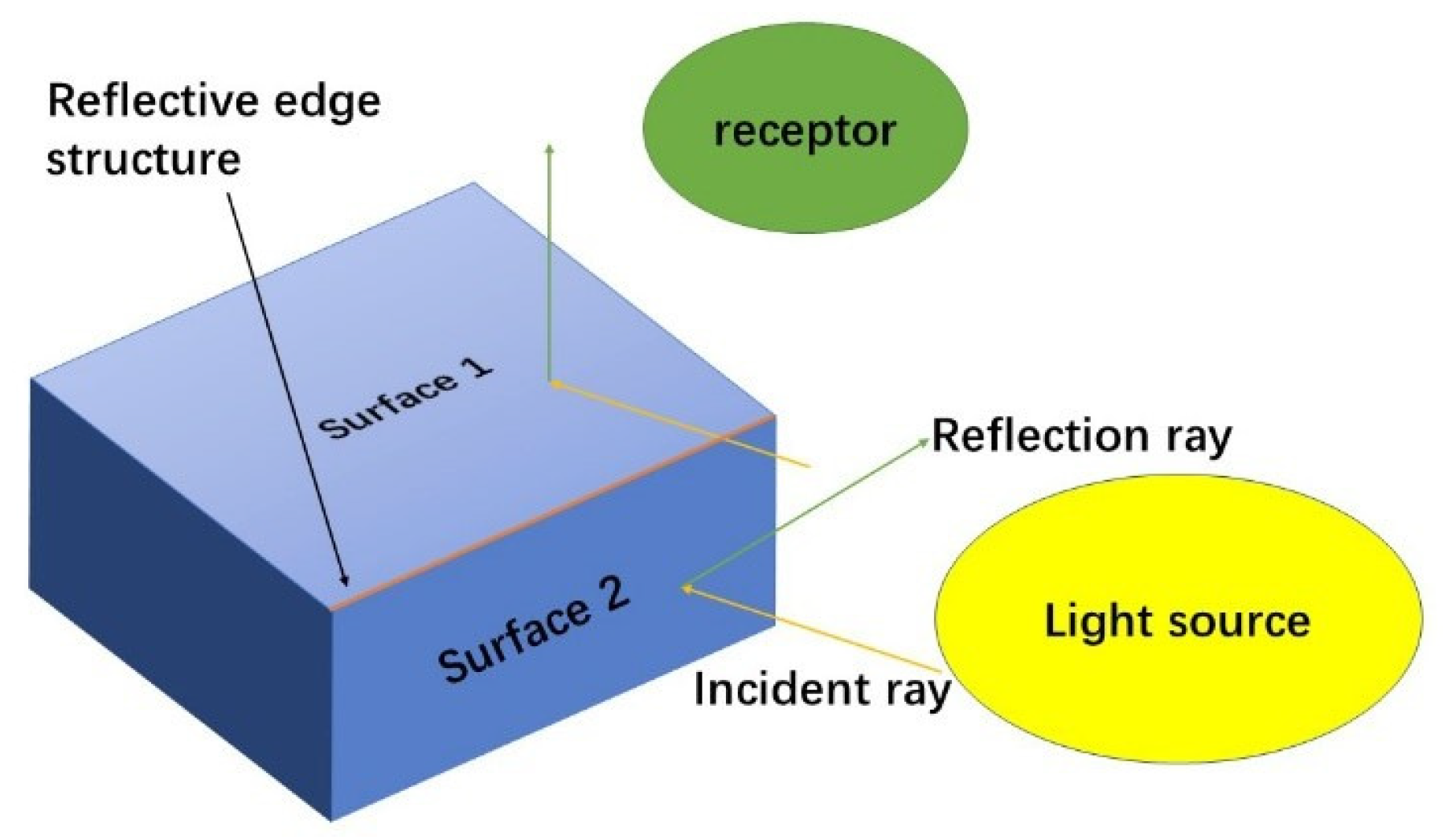
The light source is regarded as natural light or man-made light, which is expressed as $L(x,y)$ in this paper. The ’reflection ray’ is regarded as reflectance caused by a reflection of light at the boundary, which is expressed as $R(x,y)$. The receptor is a sensor, which is usually eyes or cameras. Images constructed by receptors in this paper are expressed as $I(x,y)$.

As shown in Figure 1, upon setting up a point light source, or using the sun as the light source, when the incident light from the light source exposures an object, it will reflect to the receptor. The given image $I(x,y)$ can be divided into two parts: incoming image $L(x,y)$ and reflectance $R(x,y)$. The formula is expressed as follows:

$$I(x,y)=L(x,y)\times R(x,y).$$

(12)

From Equation (12), it is clear to find that the reflectance component is a mixture in image $I(x,y)$. In order to separate the influence of incident light, restore the original features of the object (reflectance), and take the logarithm of both sides of Equation (12)

$$logI(x,y)=logL(x,y)+logR(x,y).$$

(13)

The process of the Single-Scale Retinex (SSR) algorithm is similar to the process of human visual imaging. Firstly, this algorithm uses the Gaussian kernel function to convolve the original image to achieve the information of illumination $log\left(I\right(x,y)\ast G(x,y\left)\right)$. Among them, $I(x,y)$ is the original image, and ∗ represents the convolution. The reflectance will be expressed as shown below:

$$SSR:logR(x,y)=\frac{logI(x,y)}{logL(x,y)}=logI(x,y)-log(I(x,y)\ast G(x,y)).$$

(14)

$$G(x,y)=\frac{1}{2\pi {\sigma }^2}{e}^{-\frac{x^2+y^2}{2{\sigma }^2}}.$$

(15)

where $\sigma$ is the variance (parameter of scale) of the Gaussian kernel function. When the value of $\sigma$ is small, the algorithm will extract the reflectance’s details well. On the contrary, the reflectance will be smoothed. Generally speaking, the value of $\sigma$ depends on what is required in reality.

3. The Proposed Model

3.1. Additive Bias Field

In a traditional multiplicative model, the fitting intensity of a local region must be obtained by solving the energy function’s Euler Lagrange equation. In this process, multiplication in convolution will add to the algorithm’s complexity. By inducing the Retinex theory into a multiplicative model, we can separate the reflectance and bias field from the multiplicative model. In the Euler Lagrange equation, the additive model has fewer calculations than the multiplicative model.

As mentioned above in Section 2.2, the image domain is divided into two parts. Firstly, this paper transfers the input image domain into the logarithmic domain. The $i\left(x\right)$ is regarded as the input image’s logarithmic domain, $r\left(x\right)$ is the high-frequency component, and $b\left(x\right)$ is the low-frequency component

$$\left\{\begin{array}{c}i\left(\mathbf{x}\right)=logI(x,y)\\ r\left(\mathbf{x}\right)=logR(x,y)\\ b\left(\mathbf{x}\right)=logL(x,y)\end{array}\right..$$

(16)

Formula (13) can be alternatively presented as follows:

$$i\left(\mathbf{x}\right)=b\left(\mathbf{x}\right)+r\left(\mathbf{x}\right).$$

(17)

To effectively handle images with uneven intensity, based on Formula (17), the following two hypotheses are provided as:

Hypothesis 1.

This paper divides the image domain into n disjoint local regions (in this paper, n is equal to 2), each region is described as ${\left\{{\Omega }_i\right\}}_{i=1}^n$ and the image domain is $\Omega ={\bigcup }_{i=1}^n{\Omega }_i$. Furthermore, they do not intersect with each other. Then, we assume that the bias field B changes smoothly in the local region with inhomogeneous intensity, and each disjoint local region is given a fitting function $b_j\left(\mathbf{x}\right)(j=1,\cdots ,n)$.

Hypothesis 2.

Considering the reflectance behavior characteristics of a derivative in an image domain, the Retinex theory can be fitted in the image domain. Thereinto, $b\left(\mathbf{x}\right)$ represents the inhomogeneous intensity (bias component), $r\left(\mathbf{x}\right)$ is the reflectance, which possesses the characteristics of the derivative, $i\left(\mathbf{x}\right)$ is the whole image’s logarithmic domain, and $n\left(\mathbf{x}\right)$ is the zero-mean gaussian noise. The image is modeled as follows:

$$i\left(\mathbf{x}\right)=b\left(\mathbf{x}\right)+r\left(\mathbf{x}\right)+n\left(\mathbf{x}\right).$$

(18)

3.2. The Second Derivative of the Image—Reflectance

This paper figures out the previous reflectance $r\left(\mathbf{x}\right)$. By using a Laplace operator to calculate the second derivative of the image domain, the reflection edge structure of the image domain is obtained as

$$\widehat{r}\left(\mathbf{x}\right)=▵\left(i\left(\mathbf{x}\right)\right).$$

(19)

In this sense, the following subsection will explain why the reflection edge structure can be obtained by a second-order differential calculation of the image domain.

For most images, at the boundary, which is between the target and the background, the variations of intensity are always drastic. From the first graph a in Figure 2, the first curve represents the intensity change in the image domain. In the transition process from the background image to the target, the intensity value changes from weak to strong. The red circle marked in the image denotes one of the most dramatic changes, which is the target boundary to segment.

To make this phenomenon more obvious, the gradient descent algorithm is carried out on the image to compute the first-order derivative, and the results are plotted in second graph b of Figure 2. The boundary between the background and foreground is represented as the highest point. Compared with a, the peak value at this time can clearly reflect the edge structure and the change in the trend of the image intensity.

Following the same logic, continue to take the second derivative of the graph using the Laplace operator, and the third graph c of Figure 2 is plotted. The point in the curve that crosses the zero value between the peak and the trough is the target boundary to be divided.

An image of a zebra is selected in Figure 3 to exhibit the difference between a first-order differential operator and second-order differential operator. This figure shows the effect of boundary extraction between LoG and Roberts algorithm. From the outcome, it is explicit that the LoG algorithm is stronger than Roberts algorithm.

The preprocessed edge structure $r\left(\mathbf{x}\right)$ only needs to carry out the second derivative operation in the image domain, which eliminates the partial derivative of the edge structure $r\left(\mathbf{x}\right)$ when the energy function is minimized. It eliminates the multiple convolution operation of calculating the edge structure $r\left(\mathbf{x}\right)$. Therefore, according to the above-mentioned information, our additive bias field formula is rewritten as

$$i\left(\mathbf{x}\right)=b\left(\mathbf{x}\right)+\widehat{r}\left(\mathbf{x}\right)+n\left(\mathbf{x}\right).$$

(20)

3.3. Criterion Function

According to the two hypotheses and image models proposed in Section 3.2, Formula (18) is further improved. Firstly, an initial contour line c is given as the dividing line between the two regions ${\Omega }_1,{\Omega }_2$, and the image domain $\Omega$ is divided into two parts. Since the ${\delta }_{\zeta }$ function can merely calculate the data of the very small narrow-band region attached to the boundary line c, a Gaussian truncation function $G_{\sigma }(\mathbf{x}-\mathbf{y})$ is introduced on contour line c. Define a circle with a radius of $\rho$, and the center of the circle is point $\mathbf{y}$ on the initial contour line c: $O_{\mathbf{y}}\triangleq \left\{\mathbf{x}:\left|\mathbf{x}-\mathbf{y}\right|\le \rho \right\}$. The Gaussian truncation only has values in this neighborhood, and $G(\mathbf{x}-\mathbf{y})=0$ when it goes beyond this neighborhood.

In Hypothesis 1, it is mentioned that the image domain $\Omega$ is divided into n disjoint neighborhoods ${\left\{{\Omega }_j\right\}}_{j=1}^n$, the value of n is 2 means the two regions that are inside and outside the initial contour. Using these regions, induce the partition of $O_{\mathbf{y}}$ into ${\left\{{\Omega }_j\right\}}_{j=1}^n$, as shown above ${\left\{O_{\mathbf{y}}\cap {\Omega }_j\right\}}_{j=1}^n$. Then, integrate the slowly changing bias field into each partition that has been divided as $b\left(\mathbf{x}\right),\mathbf{x}\in O_{\mathbf{y}}\cap {\Omega }_j$. Since the partition of $O_{\mathbf{y}}$ has been induced into each subregion of the image domain, the partial field is expressed as $b_j\left(\mathbf{x}\right),\mathbf{x}\in {\Omega }_j$.

3.4. Energy Function

A level set image segmentation model is proposed based on the additive bias field. To remove the influence of the reflection edge structure on the image, the $i_r\left(\mathbf{x}\right)$ is obtained as $i_r\left(\mathbf{x}\right)=i\left(\mathbf{x}\right)-\widehat{r}\left(\mathbf{x}\right)$. Referring to the clustering criterion algorithm of K-means and using the dichotomy method of the membership function, the following energy function is put forward as

$$F_{\mathbf{y}}=\sum _{j=1}^2{\int }_{O_{\mathbf{y}}}{\left|i_r\left(\mathbf{x}\right)-{\mathbf{c}}_j\right|}^2{\mu }_j\left(\mathbf{x}\right)d\mathbf{x},$$

(21)

where the ${\mu }_j\left(\mathbf{x}\right)$ is the membership function. The execution rule is described as

$$\left\{\begin{array}{cc}{\mu }_j\left(\mathbf{x}\right)& =1,\mathbf{x}\in {\Omega }_j\\ {\mu }_j\left(\mathbf{x}\right)& =0,\mathbf{x}\notin {\Omega }_j\end{array}\right..$$

Because the $b_j\left(\mathbf{x}\right)$ proposed in this paper represents the intensity fitting of the local region, the fitting value of the local regional intensity in the formula, i.e., the clustering center, is approximately expressed as ${\mathbf{c}}_j=b_j\left(\mathbf{x}\right)$. Furthermore, this formula is rewritten as

$$F_{\mathbf{y}}=\sum _{j=1}^2{\int }_{O_{\mathbf{y}}\cap {\Omega }_j}{\left|i_r\left(\mathbf{x}\right)-b_j\left(\mathbf{x}\right)\right|}^2{\mu }_j\left(\mathbf{x}\right)d\mathbf{x}.$$

(22)

Introducing the Gaussian truncation function, clustering regions $O_y\cap {\Omega }_j$ can be integrated into the area ${\Omega }_j$, and the energy value of all points x in the local region except the center point can be calculated. The redefined criteria are obtained in the following formula

$$F_{\mathbf{y}}=\sum _{j=1}^2{\int }_{{\Omega }_j}{G}_{\sigma }(\mathbf{x}-\mathbf{y}){\left|i\left(\mathbf{x}\right)-\widehat{r}\left(\mathbf{y}\right)-b_j\left(\mathbf{y}\right)\right|}^{2}d\mathbf{x}.$$

(23)

This formula only expresses the energy value of a point $\mathbf{x}$ in the local image domain, and this local image domain is a local region centered at point $\mathbf{y}$. The next step is to integrate it globally over all local regions’ centers points ${\mathbf{y}}_N(N=1,\cdots ,n)$ in the whole image domain $\Omega$, to the minimum energy $F_{\mathbf{y}}$ in the image domain $\Omega$ is obtained. The energy formula is presented as follows:

$$F=\int \left(\sum _{j=1}^2{\int }_{{\Omega }_j}{G}_{\sigma }(\mathbf{x}-\mathbf{y}){\left|i\left(\mathbf{x}\right)-\widehat{r}\left(\mathbf{y}\right)-b_j\left(\mathbf{y}\right)\right|}^{2}d\mathbf{x}\right)d\mathbf{y}.$$

(24)

In order to integrate the ${\Omega }_j$ integral area into the energy formula, the Lipschitz function is introduced, which can be used to represent two partitions of $\Omega :{\Omega }_1,{\Omega }_2$. The Lipschitz function in this paper is expressed as follows:

$$\left\{\begin{array}{cc}{\Omega }_1& :M_1\left(\phi \right)=H\left(\phi \right),{\mathrm{Contour}}^{\prime }\mathrm{s}\mathrm{outside}\hfill \\ {\Omega }_2& :M_2\left(\phi \right)=1-H\left(\phi \right),{\mathrm{Contour}}^{\prime }\mathrm{s}\mathrm{inside}\hfill \end{array}\right..$$

(25)

where $H\left(\phi \right)$ is the Heaviside function, the strength of the regional ${\Omega }_1$ value is ${\mathbf{b}}_1$, the strength of the regional ${\Omega }_2$ value is ${\mathbf{b}}_2$, and the new energy function can be obtained by exchanging the order of integration

$$E^{PRI}(\phi ,\mathbf{b})=\int \sum _{j=1}^2\left(\int G_{\sigma }(\mathbf{x}-\mathbf{y}){\left|i\left(\mathbf{x}\right)-\widehat{r}\left(\mathbf{x}\right)-b_j\left(\mathbf{y}\right)\right|}^{2}d\mathbf{y}\right)M_j\left(\phi \left(\mathbf{x}\right)\right)d\mathbf{x}.$$

(26)

According to Equation (20) proposed in this paper, the formula can be written as

$$E^{PRI}(\phi ,\mathbf{b})=\int \sum _{j=1}^2\left(\int G_{\sigma }(\mathbf{x}-\mathbf{y}){\left|i_r\left(\mathbf{x}\right)-b_j\left(\mathbf{y}\right)\right|}^{2}d\mathbf{y}\right)M_j\left(\phi \left(\mathbf{x}\right)\right)d\mathbf{x}.$$

(27)

To find the optimal solution ${\mathbf{b}}_j$ when the energy is minimized, regard $\phi$ as a fixed value and find the partial derivative of energy $E^{PRI}$ with respect to $\phi$, and make it equal to 0. Solving the derivative formula to obtain $\widehat{b_j}\left(\mathbf{x}\right)=\frac{G_{\sigma }\ast \left(i_r{M}_j\left(\phi \right)\right)}{G_{\sigma }\ast M_j\left(\phi \right)},j=1,2$, based on the Lipschitz function defined in this paper, the ${\Omega }_1$ and ${\Omega }_2$ areas of the clustering center values can be expressed as, respectively,

$$\left\{\begin{array}{cc}\hfill & \widehat{{\mathbf{b}}_1}=\frac{G_{\sigma }\ast \left(i_{r}H\left(\phi \right)\right)}{G_{\sigma }\ast \left(H\left(\phi \right)\right)}\hfill \\ \hfill & \widehat{{\mathbf{b}}_2}=\frac{G_{\sigma }\ast i_r-G_{\sigma }\ast \left(i_{r}H\left(\phi \right)\right)}{G_{\sigma }\ast 1-G_{\sigma }\ast \left(H\left(\phi \right)\right)}\hfill \end{array}\right..$$

(28)

A new local energy term $e_j$ is defined, and the regional energy term in the formula is represented by $e_j,(j=1,2)$; then, the energy function of local regions is expressed as

$$e_j\left(\mathbf{x}\right)=\int G_{\sigma }(\mathbf{x}-\mathbf{y}){\left|i_r\left(\mathbf{x}\right)-b_j\left(\mathbf{y}\right)\right|}^{2}d\mathbf{y}.$$

(29)

Expand the absolute value squared term, and write the integral multiplication as convolution

$$e_j\left(\mathbf{x}\right)={i_r}^2{1}_G-2i_r(b_j\ast G_{\sigma })+({b_j}^2\ast G_{\sigma }).$$

(30)

$1_G=\int G(\mathbf{y}-\mathbf{x})dy$ means in the region of the Gaussian truncation function is 1, and 0 outside the region. The energy term can be rewritten as

$$E^{PRI}(\phi ,b)=\int \sum _{j=1}^2{e}_j{M}_j\left(\phi \left(\mathbf{x}\right)\right)d\mathbf{x}.$$

(31)

Then, the partial derivative of energy $E^{PRI}$ with respect to $\phi$ is carried out by means of gradient descent flow to find the appropriate $\phi$ to minimize the energy term E. Take b as a fixed component, take the partial derivative of E with respect to $\phi$, and the energy driving term is obtained as

$$\frac{\partial \phi }{\partial t}=-\frac{\partial E^{PRI}}{\partial \phi }=-\delta \left(\phi \right)(e_1-e_2),$$

(32)

where $\delta \left(\phi \right)$ is the derivative of the Heaviside function, and this formula considers the inhomogeneity of image intensity on the basis of the CV model. Compared with the BC model, the time consumed by the convolution operation is reduced. In practical applications, due to the diversity of the images, the intensity difference of the images leads to $(e_1-e_2)$ great differences in the results. As a result, the robustness is poor in different images, and the time consumed in different images is uncontrollable. Hence, an activation function is added to handle data-driven items $(e_1-e_2)$.

Note that $y=arctan\left(x\right)$ is an odd function of zero crossing, and near zero, the rate of change is large, which improves the sensitivity of the small value part and makes it easy to determine the boundary. The range of the activation function is (−$\frac{\pi }{2},\frac{\pi }{2})$, so the data-driven entries are bounded between (−$\frac{\pi }{2},\frac{\pi }{2})$. This solves the problem that the data driver items of different images differ greatly. Adding an adjustable $\beta$ parameter enables data-driven items to adapt to different images, where $\beta$ is the standard deviation, increasing the robustness of the activation function. When $(e_1-e_2)$ is large, increasing the value of $\beta$ makes it closer to zero faster and determines the boundary of the target. When $(e_1-e_2)$ is small, decreasing the value of $\beta$ achieves the same effect. Finally, an adjustable energy proportionality factor $\alpha$ is added, and the original energy drive term can be rewritten as follows:

$$\left\{\begin{array}{cc}\hfill \frac{\partial \phi }{\partial t}& =-\alpha \delta \left(\phi \right)arctan\left(\frac{(e_1-e_2)}{\beta }\right)\hfill \\ \hfill \beta & =\sqrt{\frac{1}{M\times N}{\sum }_{i=1}^M{\sum }_{j=1}^N{\left(I(i,j)-\overline{I}(i,j)\right)}^2}\hfill \end{array}\right..$$

(33)

Once the gradient descent equation has been defined, the next procedure is evolution. Consider the evolution process of the level set function

$${\phi }^{n+1}={\phi }^n+▵t·\left(\frac{\partial \phi }{\partial t}\right).$$

(34)

Thereinto, $▵t$ is a time step, and $\frac{\partial \phi }{\partial t}$ has been defined in Equation (33).

3.5. Regularization Function and Smoothing Method of Level Set Function

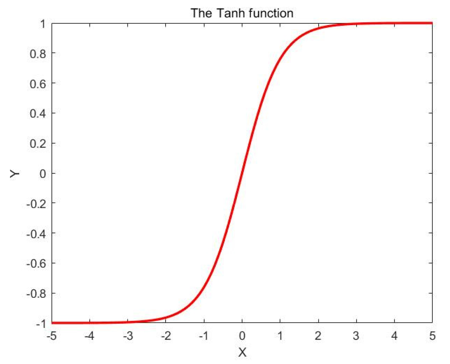
The regularization function used in this paper is Equation (35) whose function curve is presented in Figure 4:

$${\phi }_R=tanh\left(\eta {\phi }^{n+1}\right).$$

(35)

In this formula, $\eta$ is an invariant quantity, the regularization function is used to increase the slope of the zero-crossing segment, which can quickly stretch the level set function near zero to the $\pm c_0$ value and restrain the rate of change near the $\pm c_0$ value. It tends to flatten out as it pushes toward the asymptote $y=\pm c_0$ line. In this paper, a similar length term plays the role of a smooth contour, i.e., the neighborhood average filtering algorithm is used for $\phi$ as

$${\phi }_L\left(\mathbf{x}\right)=mean\left({\phi }_R\left(\mathbf{y}\right)\right|y\in {\Omega }_{\mathbf{x}}),$$

(36)

where ${\phi }_L\left(\mathbf{x}\right)$ refers to the intensity value of point $\mathbf{y}$ on the level set. ${\Omega }_{\mathbf{x}}$ refers to the image domain centered on $\mathbf{x}$, $\omega$ is the radius of the window area, whose size is $\omega \times \omega$. $mean(·)$ represents calculating the average intensity within the window.

3.6. Position of Initial Contour

Although our model is robust to the initial contour, the initial contour in two cases will lead to a great segmentation challenge:

The first case: The initial contour does not intersect with the segmentation target. In this case, the segmentation result will contain many meaningless segmentations, and the position of this initial contour will become stuck in a false boundary because of background information.

The second case: This case most likely happens when segmenting big targets in which the original image is divided into left and right or up and down regions. The initial contour is set outside the target, but it intersects with one side of the target’s boundary. In this case, the level set cannot evolve to another side of the target’s boundary, and the level set will be trapped in the local optimal solutions.

In conclusion, the position of the initial contour is usually set inside the target or set to contain the target. If the initial contour is set outside the target, we should ensure that the intersection accounts for a large proportion of the initial contour.

4. Algorithm Steps and Datasets

The detailed steps of the PFR model are shown in Algorithm 1; n are the maximum iterations; $\sigma ,{\sigma }_R,\alpha ,k,\omega$ are all parameters utilized in later experiments.

Unless otherwise noted, the parameters of the proposed model have been set as mentioned in Algorithm 1. The variance parameters of the Speckle noise and Salt and Pepper noise are 0.04 and 0.05, respectively. The experiment is run with MatlabR2020a software, and the computer processor parameters are: 2.9 GHz AMD Ryzen 7. Default: the red line in the image is the result of the segmentation, and the green line is the initial contour line.

The images segmented in the below experiments are mainly from Berkeley Segmentation Datasets: https://www2.eecs.berkeley.edu/Research/Projects/CS/vision/bsds/ (accessed on 24 September 2022).

Algorithm 1 Pre-fitting reflectance (PFR) for image segmentation

Output: The given images with different objects, parameters $c_0,\sigma ,{\sigma }_R,\alpha ,k,▵t,n$.

Ensure: Segmentation results with final contours.

1: Initialization: set fixed values for parameters $c_0=1,▵t=1$, set default values for parameters $\sigma =4,{\sigma }_R=2,\alpha =2,k=7,\omega =9,n=50$ which can be adjusted according to different situations. (Thereinto, $\sigma$ is the radius of the gaussian kernel function, ${\sigma }_R$ is the variances of the gaussian kernel function, $\alpha$ is the coefficient of data-driving term, k is the coefficient of smoothing-term, $\omega$ is the radius of the gaussian kernel function, n is the number of iterations.) Initialize the level set function (${\Omega }_1$ is the whole image domain, ${\Omega }_2$ is the domain in contour, $\partial {\Omega }_2$ is the contour) as $\varphi (\mathbf{x},t=0)=\left\{\begin{array}{cc}-c_0,& \mathbf{x}\in {\Omega }_2-\partial {\Omega }_2\hfill \\ 0,& \mathbf{x}\in \partial {\Omega }_2\hfill \\ c_0,& \mathbf{x}\in {\Omega }_1-{\Omega }_2\hfill \end{array}\right.$. 2: The image domain is transformed to gray image, and the logarithmic transformation of gray image domain is carried out to obtain the logarithmic domain of the image. 3: for$i\leftarrow 1$to$\mathrm{n}$do 4:    Compute the $\widehat{b_1}$ and $\widehat{b_1}$ with Equation (28). 5:    Formulate the data driving term as Equation (33). 6:    Compute the level set function evolution with Equation (34). 7:    if $\left|{\varphi }^{i+1}-{\varphi }^i\right|\le \epsilon$ then       End iteration. 8:    else       Regularize level set function ${\phi }^i$ as Equation (35).    end if 9: end for 10: Compute the average filtering method with Equation (36). 11: Return segmentation result $\left|{\varphi }^{i+1}-{\varphi }^i\right|\le \epsilon$ with final contours.

5. Experimental Results and Relative Analysis

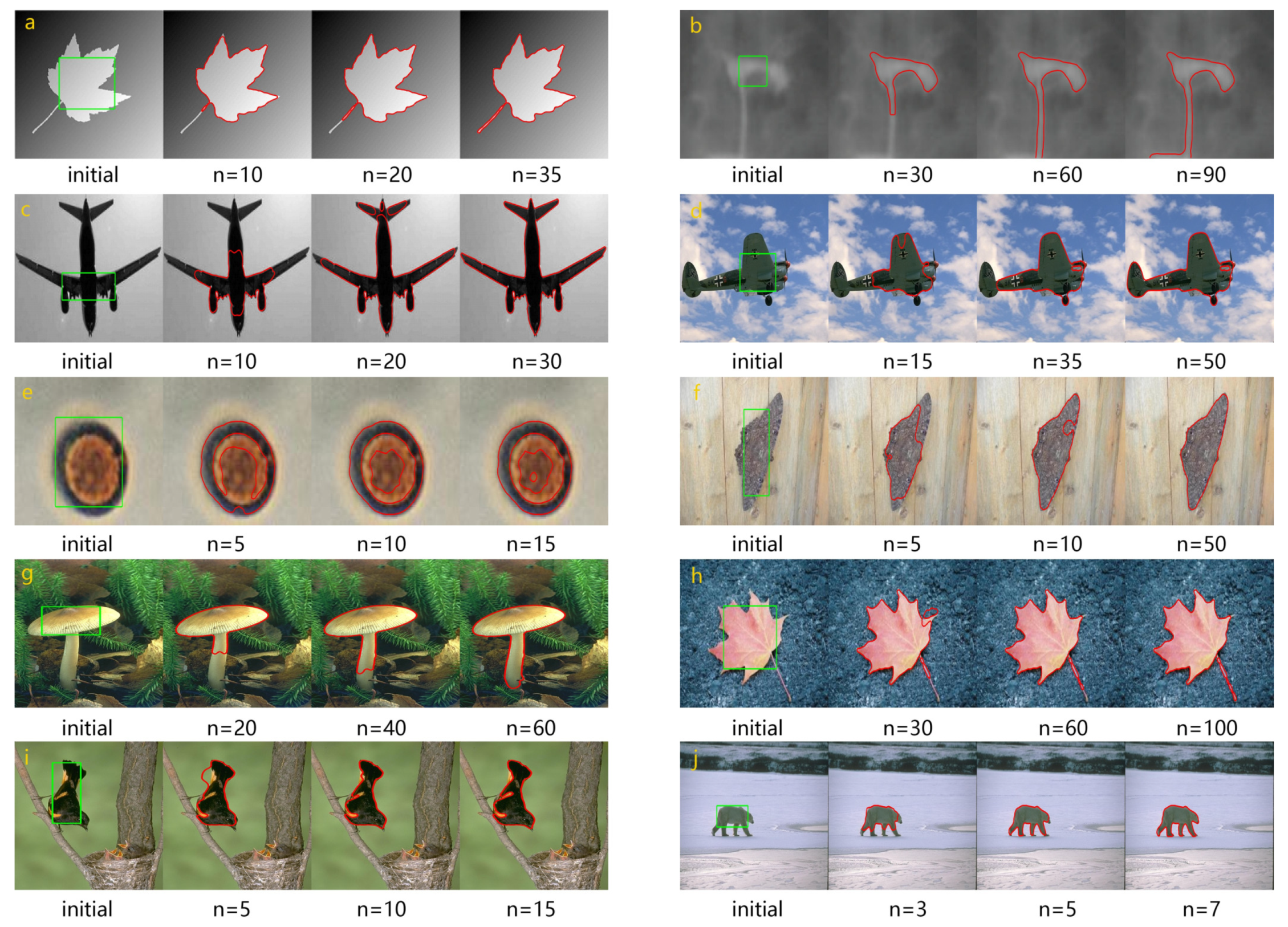
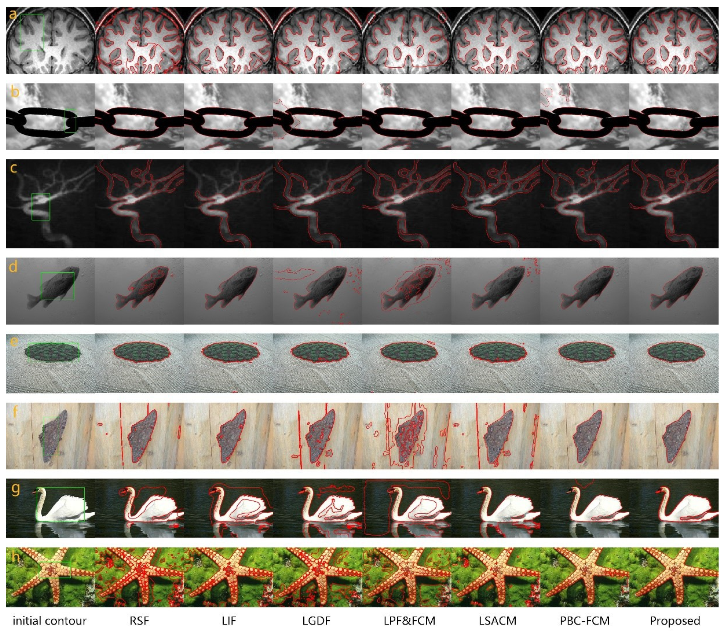
In order to verify the feasibility of the proposed model, the authors show the segmentation process of the proposed model and the effect diagram in the following sections. We presented the process of segmentation in Figure 5 and listed the hyper-parameters in

Table 1. The parameters of the experiments in Figure 5 of the proposed model.

Image/Parameters	$\mathit{\sigma }$	${\mathit{\sigma }}_{\mathit{R}}$	$\mathit{\omega }$	k	$\mathit{\alpha }$
a	6	1.5	15	5	2
b	4	1	9	7	3
c	8	1.5	25	6	1.5
d	9	1.5	11	14	1.5
e	4	1	10	8	2.5
f	3.5	1.5	11	15	2.5
g	5.5	1.5	13	13	1.5
h	4	1.2	9	7	1.5
i	9	2.5	25	13	1.5
j	5	2	17	6	2.5

. Besides, six traditional models are compared with the proposed model, and the segmentation results are presented in Figure 6. The results make a line diagram in Figure 7 of the time spent dividing each image between each comparison model and the proposed model, which more intuitively reflects the high efficiency of the proposed model, RSF, LIF, LGDF, LPF-FCM, LSACM, and PBC-FCM. The proposed model can accurately and quickly segment the images that cannot be perfectly segmented by other models, or even the images that are poorly segmented by other models, which strongly proves the segmentation ability of the proposed model.

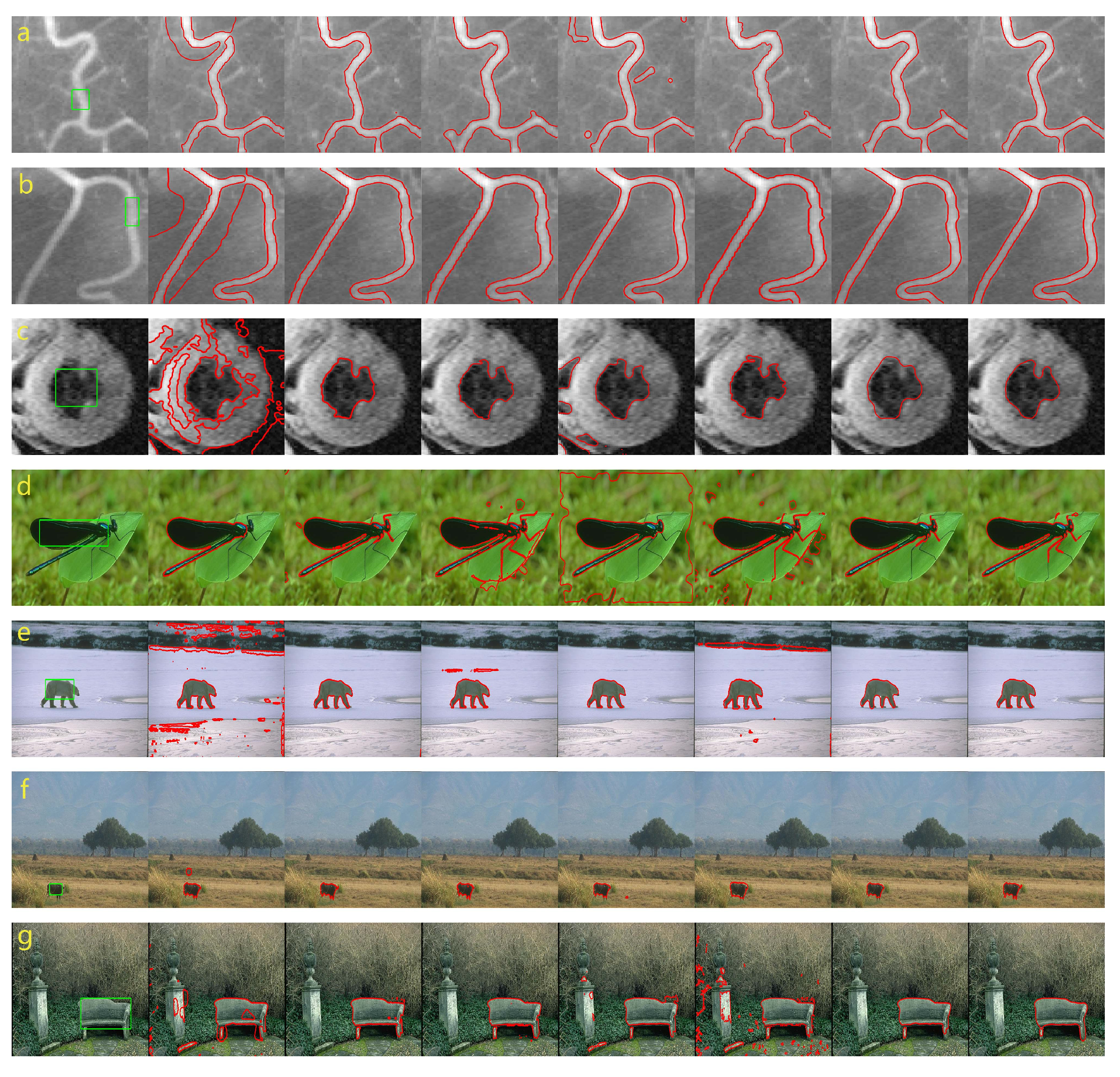
The next step is the comparative test of accuracy. A total of seven pictures are selected, the same initial contour is set and all models can be run. Finally, the results of the comparative experiment are shown in Figure 8. The running time, the number of iterations and accuracy of each model (intersection over union and intersection over union “1”) are shown in

Table 2. The datum of spent time and IOU of segmentation results by seven ACMs under the same initial contour in Figure 8. The first value is time(s) and the second value is IOU.

Model	Image a	Image b	Image c	Image d	Image e	Image f	Image g
RSF	2.42/0.396	7.92/0.256	8.24/0.146	46.3/0.854	0.41/0.340	12.0/0.751	43.9/0.646
LIF	5.03/0.809	8.83/0.953	0.27/0.874	24.1/0.861	3.15/0.903	1.31/0.867	1.97/0.876
LGDF	4.47/0.861	6.41/0.898	0.13/0.895	9.51/0.759	1.13/0.866	0.30/0.667	2.70/0.906
LPF and FCM	7.11/0.811	3.35/0.935	5.05/0.611	55.8/0.404	14.6/0.920	6.27/0.849	7.31/0.793
LSACM	6.61/0.862	7.92/0.857	5.79/0.878	45.2/0.757	12.9/0.542	4.53/0.813	16.6/0.618
PBC and FCM	1.68/0.895	2.18/0.942	1.04/0.783	7.71/0.872	8.47/0.915	3.64/0.857	2.62/0.855
Proposed	0.54/0.911	0.75/0.955	0.05/0.911	1.49/0.895	0.24/0.941	0.09/0.903	0.81/0.902

and

Table 3. The data of iterations about results of the experiments by seven ACMs under the same initial contour in Figure 8.

Model	Image a	Image b	Image c	Image d	Image e	Image f	Image g
RSF	100	500	500	1100	10	200	1100
LIF	1100	2000	10	200	30	12	30
LGDF	500	900	7	80	10	5	50
LPF and FCM	400	160	150	500	90	80	100
LSACM	400	120	250	90	30	50	90
PBC and FCM	200	320	100	400	100	90	80
Proposed	100	150	5	60	7	6	20

. The concept of IOU is defined as

$$IOU=\frac{B_1\cap B_2}{B_1\cup B_2}.$$

(37)

Intersection over union is a concept used in object detection. IOU calculates the intersection rate of “predicted borders” and “real borders”—the ratio of their intersection and union. Here, $B_1$ and $B_2$ is the “predicted borders” and “real borders”, respectively. Ideally, they overlap completely, so the ratio is one.

5.1. The Segmentation Results and Processes of Eight Images with Different Types

In this section, 10 images with uneven illumination, inhomogeneous intensity, low contrast, weak boundary or bias field are selected to perform target segmentation experiments with PFRACM. From a and c of Figure 5, gray images with uneven illumination are selected; from b of Figure 5, it can be seen that medical images with a strong bias field, weak boundary and no obvious contrast are selected. Figure 5d–j are colorful images in the real world. In the segmentation process, these images easily fall into a false boundary due to the uneven intensity or illumination of the background, so the image segmentation performance is not so good.

The parameters of Section 5.1 are shown in Table 1. The n in Figure 5 below each image represents the number of iterations. The experimental results are divided into ten groups and shown in Figure 5, in which each group is composed of the initial contour, two rows of the evolution process and the segmentation results. The satisfactory results indicate that the quality of segmentation is optimal. Specifically, the proposed model is capable of segmenting images with uneven intensity that are difficult to segment for former ACMs.

5.2. Comparison of Time Consumption

In this section, to compare the segmentation time of PFRACM with some classic region-based models, including RSFACM, LIF, LGDF, LPF and FCM, LSACM, PBC-FCM, eight images from a–h were chosen to prove that PFRACM has an optimal segmentation speed.

Figure 6 shows the comparisons of PFRACM and other mentioned ACMs under precise conditions with the same initial contours. In Figure 6, the first column presents the original images and initial contours. The second column to the last column presents the segmentation results of the RSFACM, LIFACM, LGDF, LSACM, PBC-FCM, respectively. The consumption time of each image segmented by PFRACM and other mentioned ACMs make up a line chart presented in Figure 7. Among them, RSFACM, LSACM will figure out at least four times the convolution in each iteration; thus, the time consumed is significantly more than the other model. In addition, it is not hard to see that PFRACM’s efficiency is higher than other ACMs because the additive model has few calculations, and the reflectance is figured out before iterations and the optimized regularization term. From Figure 7, PBC and FCM also have higher efficiency because of its pre-fitting local intensity by the FCM algorithm. However, its segmentation quality depends heavily on the initial contour. Thus, under the premise of achieving optimal segmentation results, the PFRACM is superior to PBC and FCM.

5.3. Comparison of Segmentation Quality of Different Models

In this section, we select seven images from a–g segmented by RSFACM, LIFACM, LGDF, LPF and FCM, LSACM and PFRACM to demonstrate that the proposed model has higher quality segmentation than other mentioned models. Table 2 shows the segmentation time and precision. In this data obtained from Figure 8, it is distinctly noticed that the precision segmented by PFRACM is superior to other models. Furthermore, combined with Figure 7, the time consumption recorded in Table 2 displays that PFRACM is equipped to achieve the optimal segmentation and possesses a higher efficiency than other models.

In Table 3, the data recorded are the iteration numbers of each image. Without setting larger $▵t$ and $\alpha$, PFRACM still segments models with fewer iterations than the mentioned models. Fewer iterations signifies fewer computations. In this sense, we can draw a conclusion that PFRACM can segment images more accurately and quickly than the six other outstanding ACMs.

5.4. Robustness of Initial Contour of the Proposed ACM

From Figure 9, eight images with uneven intensity and false boundaries that were difficult to separate were selected to discuss the robustness of the initial contour. In A, real world images with relatively complex grayscale features were selected. In b–h, seven medical images were selected, and the green line represents the initial contour, while the red line represents the segmentation result. Accuracy comparison tests are carried out on these 4 × 8 = 32 images, and the accuracy of the datum are shown in

Table 4. The datum of spent time and IOU of segmentation results by PFR under the different initial contours in Figure 9. The first value is time (s), and the second value is IOU.

	Image a	Image b	Image c	Image d	Image e	Image f
Initial 1	3.73/0.903	0.72/0.955	0.23/0.550	0.48/0.911	1.91/0.904	0.53/0.961
Initial 2	3.75/0.903	0.72/0.955	0.23/0.549	0.47/0.911	1.94/0.904	0.53/0.961
Initial 3	3.72/0.903	0.70/0.955	0.23/0.549	0.48/0.911	1.87/0.904	0.52/0.961
Initial 4	3.70/0.903	0.71/0.955	0.23/0.550	0.48/0.911	1.93/0.904	0.52/0.961

. Combined with Figure 9 and the outcomes in Table 4, it follows that different initial contour lines have no substantial influence on the segmentation accuracy, segmentation time and iteration times of the energy function of the proposed model. In the energy driving process guided by different initial contour lines, optimal segmentation results can still be obtained at the end.

5.5. Experiments and Analysis of the Noise-Robustness of the Proposed Model

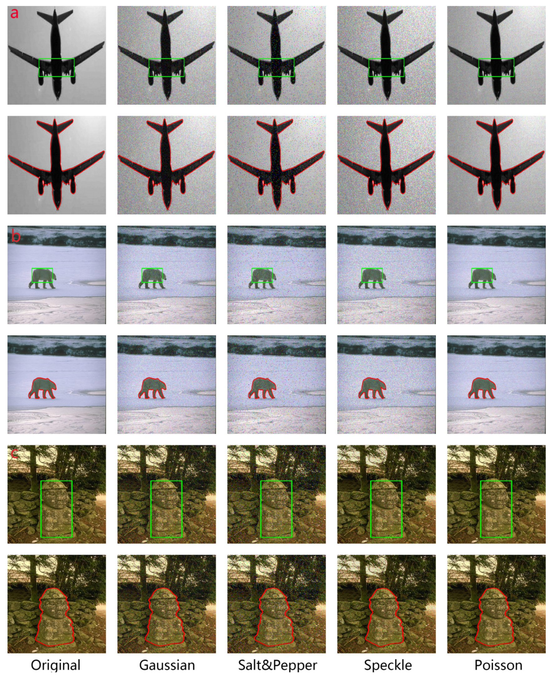
In this section, one grayscale and two colorful images were selected to test the robustness of the proposed model in the case of being corrupted by the noise of Gaussian, Salt and Pepper, Speckle and Poisson, and the coefficients of noise are obtained from Section 4. These three images all have the properties of strong uneven illumination and intensity, and it is difficult to obtain satisfactory segmentation results for some other models without any noise.

In Figure 10, three images are corrupted by Gaussian, Salt and Pepper, Speckle and Poisson noise segmented to compare with segmentation without noise. In Figure 10, six rows have been divided into three groups, each group includes the original image with the initial contour and segmentation results. To guarantee the fairness, each image in the same group has been set to the same initial contour. Consumption time and segmentation quality are recorded in

Table 5. The datum of spent time and IOU of segmentation results under the different noise-corrupted in Figure 10. The first value is time (s), and the second value is IOU.

	Image a	Image b	Image c
Non-noise	1.46/0.937	0.41/0.940	0.91/0.957
Gaussian	1.49/0.939	0.43/0.929	0.95/0.957
Salt and Pepper	1.47/0.938	0.40/0.940	1.08/0.958
Speckle	1.45/0.937	0.35/0.929	0.84/0.948
Poisson	1.57/0.940	0.35/0.936	0.86/0.960

. Owing to the fact that reflectance is pre-fitted by the LoG algorithm, which has the function of smoothing, the noise can hardly influence the segmentation. Furthermore, it is noticeable in Section 4 that PFRACM includes the step of the logarithmic image domain, which will decrease the effect caused by discrete high-frequency noise. Last but not the least, by adjusting the ${\sigma }_R$ or $\omega$, the model can adapt to varying noise.

5.6. Experiments and Analysis on the Low-Contrast and Blurred Images

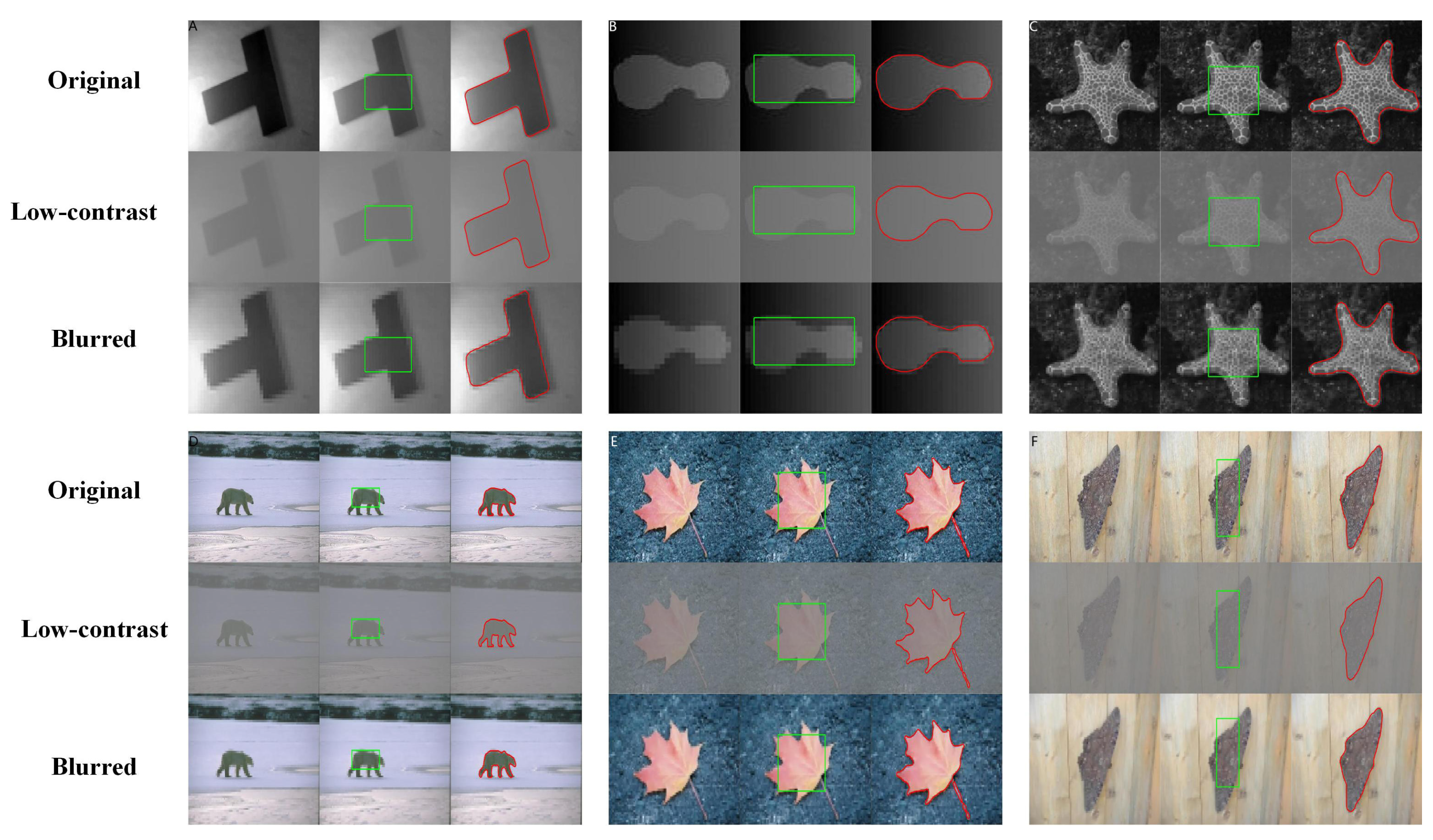
Apart from the noise, low-contrast and blurred images will also bring big challenges to image segmentation. Objects in low-contrast images express an indistinct boundary feature and blurred images will smooth the difference between the reflectance and background. Both these two cases will interfere with the process of image segmentation.

In this section, to verify that our model is robust to low-contrast and blurred images, six images (four gray-scale images and two color images) were selected to segment. This part keeps the position of the initial contour and parameters invariant, only changing the input image. These images are divided into six groups (from A to F), each group has original image segmentation, low-contrast image segmentation and blurred image segmentation. The datum of spent time and IOU of results are presented in

Table 6. The data of spent time and IOU of segmentation results in each group in Figure 11 under different input images (original, low-contrast and blurred). The first value is time (s), and the second value is IOU.

	Group A	Group B	Group C	Group D	Group E	Group F
Original	0.27/0.98	0.04/0.99	0.64/0.90	0.40/0.94	1.04/0.95	0.44/0.98
Low-contrast	0.26/0.96	0.04/0.99	0.69/0.90	0.42/0.92	1.12/0.95	0.45/0.98
Blurred	0.28/0.95	0.05/0.96	0.71/0.89	0.48/0.88	1.20/0.89	0.52/0.96

.

From Figure 11, although the low-contrast image has been set to below the original image at 80% contrast and the blurred images have been fuzzed by mosaic in five kernel sizes, our model still achieves a satisfactory result as before. Combined with the datum in Table 6, it is explicit that the time consumed and accuracy is very close to the optimal value.

As mentioned above, it can be concluded that the PFR model is robust to low-contrast and blurred images.

5.7. Experiments and Analysis of the Data-Driving Term

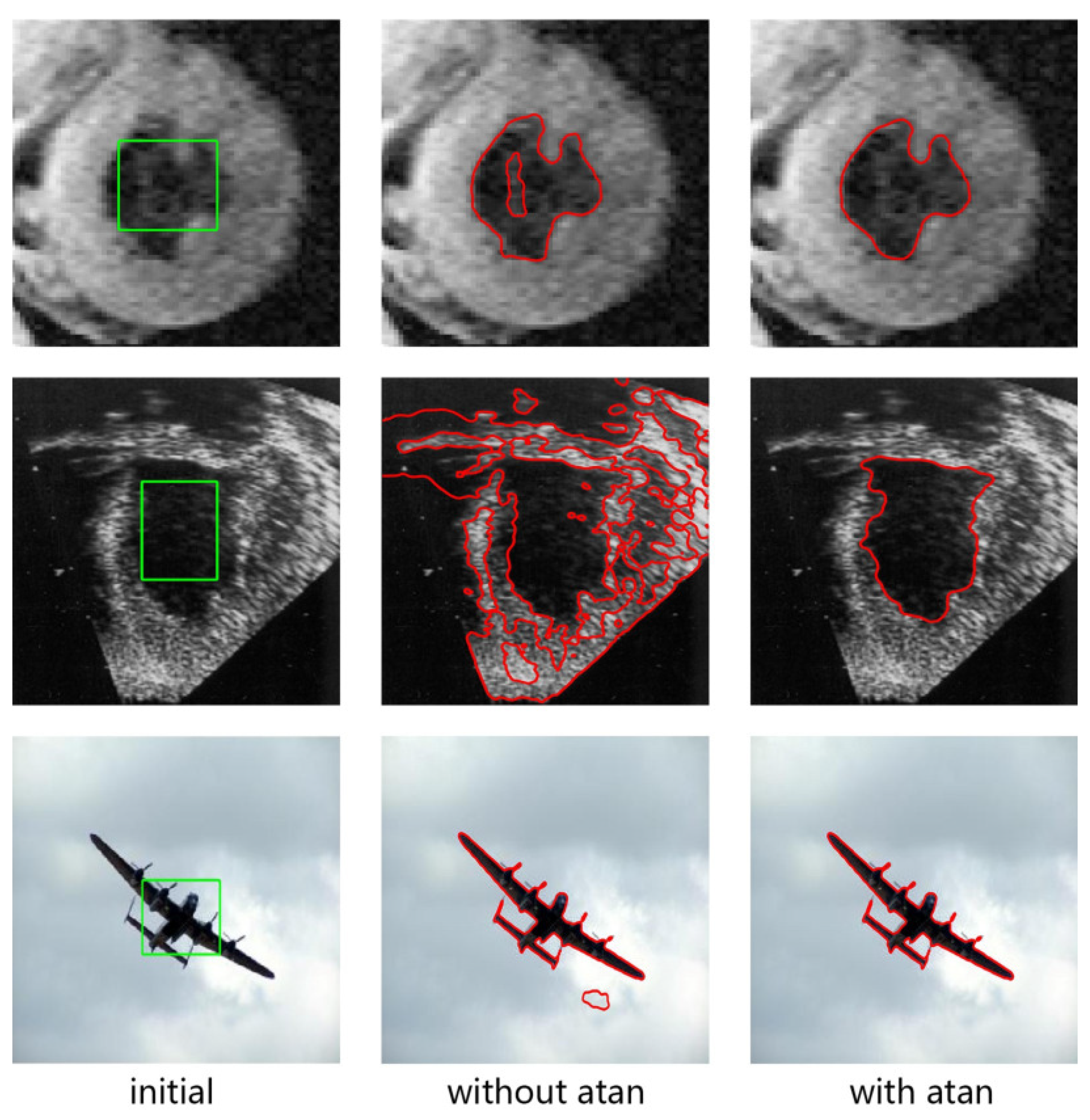
As mentioned in Section 3.4, the data-driving term in this paper adds an activation function $arctan(·)$. The activation function is applied to limit the difference domain between inner and outer intensity. The characteristic of this activation function is that it is sensitive to intensity difference when the value is located near zero. While the intensity difference is obvious enough, the activation function will weaken the effect produced by large differences, such as a penalty term. The impact of this activation function is that the optimal solution of the level set function will not be trapped in the error boundary because the gradient descent’s momentum is too large for evolution.

This part chooses two grayscale images and one colorful image to proceed with the ablation experiments. The experimental results are presented in Figure 12. The first column displays the position of the initial contour and original image. The second column displays the segmentation results without the activation function of $arctan(·)$, and the third column displays the segmentation results with the activation function of $arctan(·)$. It is obvious that the activation function can effectively reduce meaningless segmentation and greatly improve the quality of segmentation.

5.8. Segmentation of Dual-Objective (or Multi-Objective) Images with Different ${\sigma }_R$

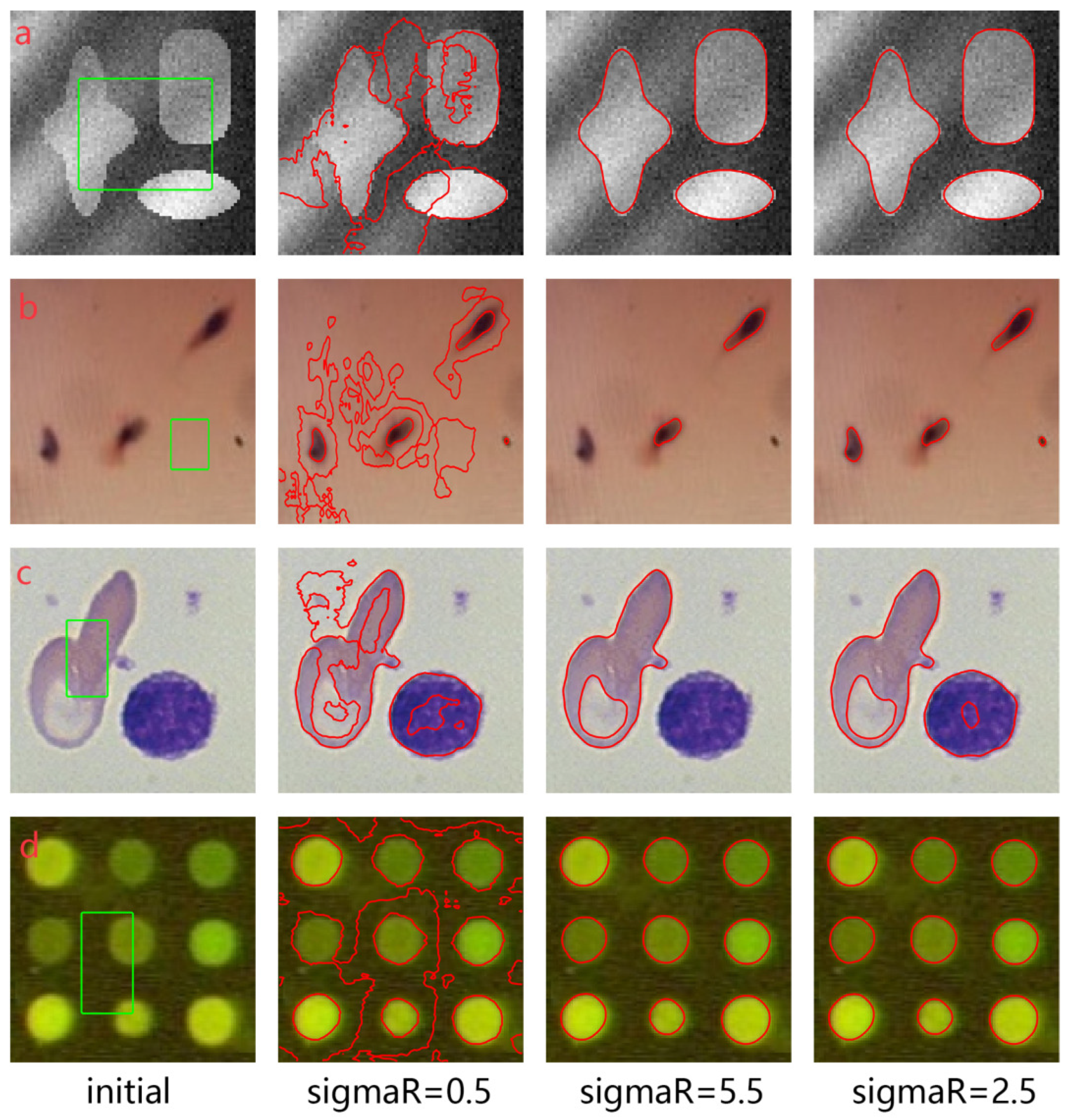
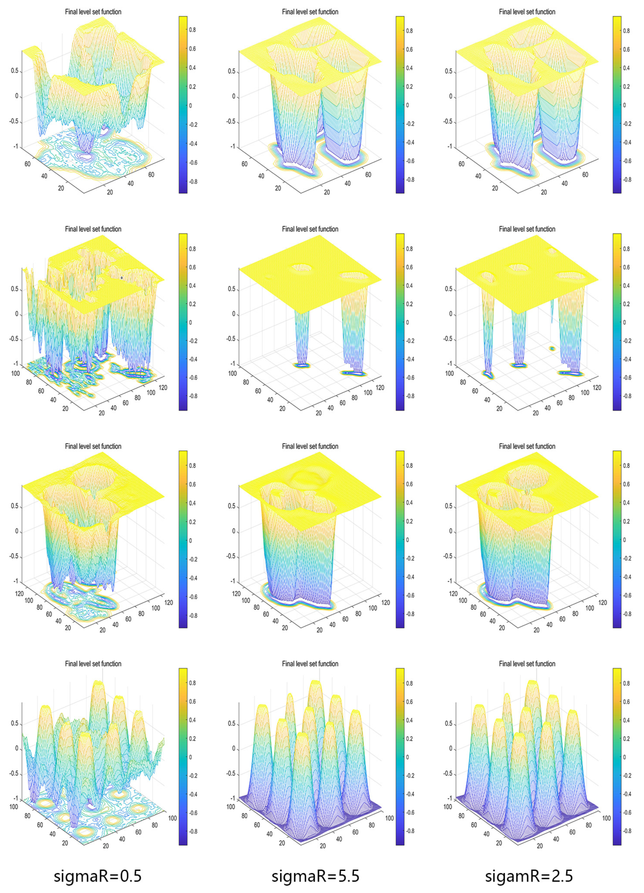
In this section, four images with dual-objective or multi-objective segmentation are selected to demonstrate the capacity of multi-objective segmentation with our model and three various parameters, which are the variance of the LoG algorithm, to determine the ability to smooth images. When ${\sigma }_R$ is equal to 0.5, the gaussian filter can enhance the characteristics in the image vastly. Hence, form the 2nd column, results show that the contour curve is stuck in the mendacious boundary. When the ${\sigma }_R$ is equal to 5.5, the capacity of smoothing is strengthened, and then, some vague targets, small targets or some targets whose intensity is in proximity to the background will be smoothed by the gaussian filter. In other words, the boundary characteristic may be eliminated. From the 3rd column, this deduction can be confirmed. From the 4th column, the desired outcome is obtained, so the appropriate value of ${\sigma }_R$ is 2.5 in multi-objective segmenting for our model. At the end of this section, the consequences of the segmentation are shown in Figure 13 and the three-dimensional reflection of intensity changes will be shown in Figure 14. The other hyper-parameters in this experiment are listed in

Table 7. The parameters of the proposed model when segmenting these four images in Figure 13.

	$\mathit{\sigma }$	$\mathit{\alpha }$	n	k	$\mathit{\omega }$
Image a	4	1.5	50	7	9
Image b	1.5	3	150	5	15
Image c	3	2	150	10	15
Image d	6	2	35	8	15

.

5.9. Comparison of Accuracy of Roberts Operator and LoG

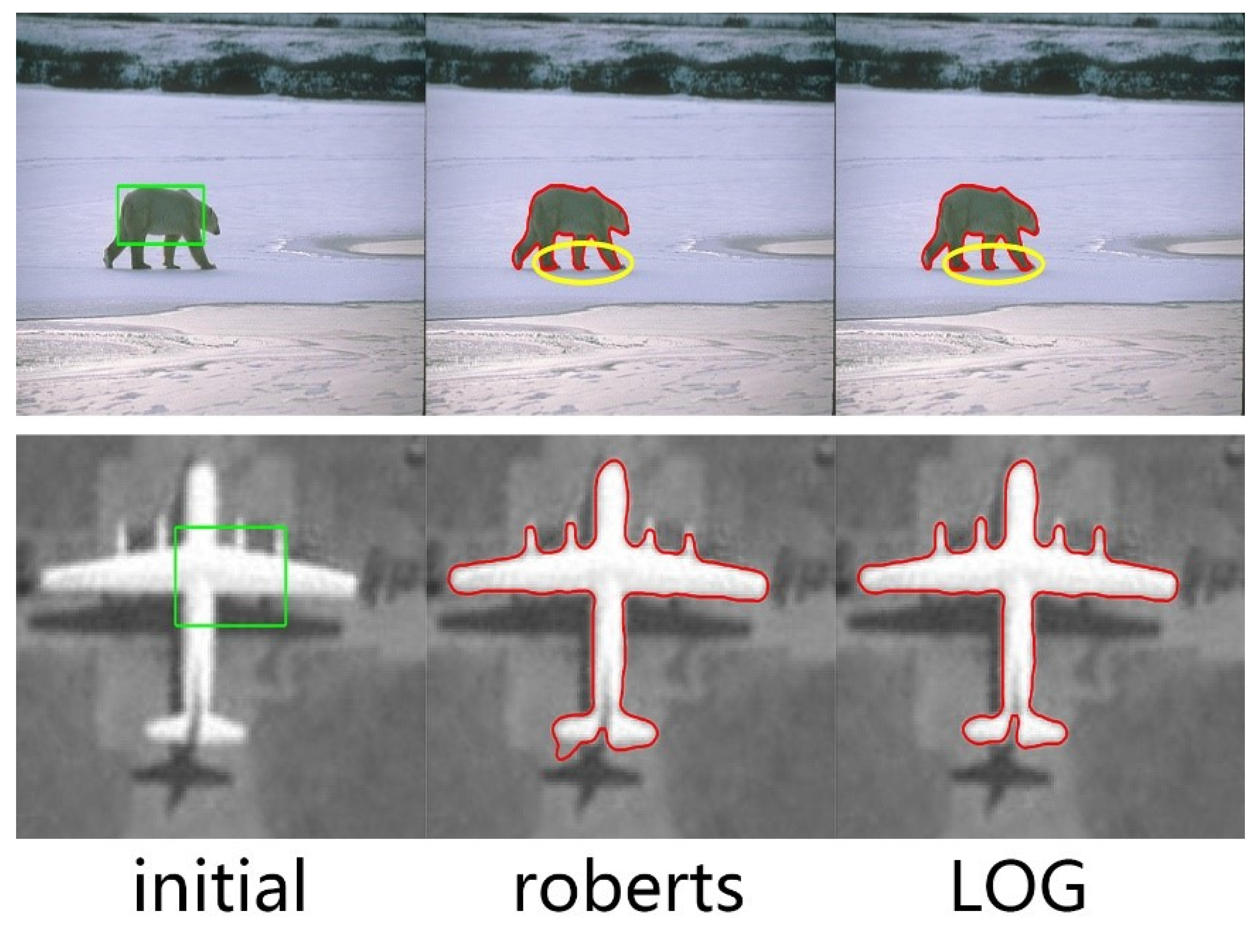
In this part, the authors choose two images with uneven intensity and use the LoG algorithm and Roberts operator to calculate the pre-fitted $\widehat{r}$, respectively. The results are shown in Figure 15, and the comparisons of time consuming and segmentations’ accuracy are presented in

Table 8. The data of spent time and IOU of results under the Roberts operator and LoG operator in Figure 15. The first value is time (s), and the second value is IOU.

	Roberts Operator Time(s)/IOU	LoG Time(s)/IOU
bear	0.19/0.937	0.17/0.941
plane	0.59/0.937	0.57/0.983

. From the segmentation results and table data, compared with the Roberts operator, the LoG algorithm can better highlight the edge structure. (The yellow line is set to highlight the differences between the two images).

5.10. Conclusions and Future Work

In this paper, the authors propose a robust active-contour model based on the pre-fitting reflectance and Retinex theory. Firstly, this paper applies the Retinex to reconstruct the image domain. Secondly, by utilizing the LoG algorithm to pre-fit the reflectance before iterations, this step saves a lot of time in iterations. Thirdly, this paper applies a new activation function in data-driving terms, and this step effectively improves the quality of segmentations. From the above experimental results and analysis, it can be concluded that the PRF model achieves a satisfactory effect both on speed, robustness and segmentation quality.

In future research, based on the work of [34,35,36], the authors will consider applying different distance measurements to substitute the Euclidean distance. The authors will also consider proposing multi-phase ACM to segment objects with different colors. From the perspective of measuring distance, we will consider studying the convex optimization of an active contour model based on different distance measures and attempt to substitute other measuring rules (Canberra metric, Tanimoto measure, Kullback–Leibler divergency and Jeffrey divergency, etc.) for Euclidean distance to construct the energy function. Furthermore, the authors will apply methods of machine-learning [38,39] to automatically calibrate parameters and optimize the final segmentation results and use a generative adversarial network (GAN) [40] to enhance the amount of template data to achieve better segmentation results.

References

1. Kolev, K.; Klodt, M.; Brox, T.; Cremers, D. Continuous Global Optimization in Multiview 3D Reconstruction. Int. J. Comput. Vis. 2009, 84, 80–96. [Google Scholar] [CrossRef] [Green Version]
2. Liu, Y.; He, C.; Wu, Y. Variational model with kernel metric-based data term for noisy image segmentation. Digit. Signal Process. A Rev. J. 2018, 78, 42–55. [Google Scholar] [CrossRef]
3. Choy, S.K.; Yuen, K.; Yu, C. Fuzzy bit-plane-dependence image segmentation. Signal Process. 2019, 154, 30–44. [Google Scholar] [CrossRef]
4. Chen, Y.; Jiang, W.; Charalambous, T. Machine learning based iterative learning control for non-repetitive time-varying systems. Int. J. Robust Nonlinear Control 2022. Early View. [Google Scholar] [CrossRef]
5. Chen, Y.; Zhou, Y.; Zhang, Y. Machine learning-based model predictive control for collaborative production planning problem with unknown information. Electronics 2021, 10, 1818. [Google Scholar] [CrossRef]
6. Rao, Y.; Ni, J.; Xie, H. Multi-semantic CRF-based attention model for image forgery detection and localization. Signal Process. 2021, 183, 108051. [Google Scholar] [CrossRef]
7. Kaur, K.; Jindal, N.; Singh, K. Fractional Fourier Transform based Riesz fractional derivative approach for edge detection and its application in image enhancement. Signal Process. 2021, 180, 107852. [Google Scholar] [CrossRef]
8. Caselles, V.; Catté, F.; Coll, T.; Dibos, F. A geometric model for active contours in image processing. Numer. Math. 1993, 66, 1–31. [Google Scholar] [CrossRef]
9. Li, C.; Xu, C.; Gui, C.; Fox, M.D. Distance regularized level set evolution and its application to image segmentation. IEEE Trans. Image Process. 2010, 19, 3243–3254. [Google Scholar] [CrossRef]
10. Mumford, D.; Shah, J. Optimal approximations by piecewise smooth functions and associated variational problems. Commun. Pure Appl. Math. 1989, 42, 577–685. [Google Scholar] [CrossRef]
11. Chan, T.F.; Vese, L.A. Active contours without edges. IEEE Trans. Image Process. 2001, 10, 266–277. [Google Scholar] [CrossRef] [PubMed] [Green Version]
12. Biswas, S.; Hazra, R. A level set model by regularizing local fitting energy and penalty energy term for image segmentation Soumen. Signal Process. 2021, 183, 108043. [Google Scholar] [CrossRef]
13. Li, C.; Kao, C.-Y.; Gore, J.C.; Ding, Z. Minimization of region-scalable fitting energy for image segmentation. IEEE Trans. Image Process. 2008, 17, 1940–1949. [Google Scholar] [PubMed] [Green Version]
14. Wang, L.; He, L.; Mishra, A.; Li, C. Active contours driven by local Gaussian distribution fitting energy. Signal Process. 2009, 89, 2435–2447. [Google Scholar] [CrossRef]
15. Zhang, K.; Song, H.; Zhang, L. Active contours driven by local image fitting energy. Pattern Recognit. 2010, 43, 1199–1206. [Google Scholar] [CrossRef]
16. Jin, R.; Weng, G. Active contour model based on improved fuzzy c-means algorithm and adaptive functions. Comput. Math. Appl. 2019, 78, 3678–3691. [Google Scholar] [CrossRef]
17. Szilagyi, L.; Benyo, Z.; Szilágyi, S.M.; Adam, H.S. MR brain image segmentation using an enhanced fuzzy c-means algorithm. In Proceedings of the 25th Annual International Conference of the IEEE Engineering in Medicine and Biology Society, Cancun, Mexico, 17–21 September 2003; Volume 1, pp. 724–726. [Google Scholar]
18. Ding, K.; Xiao, L.; Weng, G. Active contours driven by local pre-fitting energy for fast image segmentation. Pattern Recognit. Lett. 2018, 104, 29–36. [Google Scholar] [CrossRef]
19. Wang, X.F.; Min, H.; Zhang, Y.G. Multi-scale local region based level set method for image segmentation in the presence of intensity inhomogeneity. Neurocomputing 2015, 151, 1086–1098. [Google Scholar] [CrossRef]
20. Wang, H.; Huang, T.Z.; Xu, Z.; Wang, Y. A two-stage image segmentation via global and local region active contours. Neurocomputing 2016, 205, 130–140. [Google Scholar] [CrossRef]
21. Niu, S.; Chen, Q.; de Sisternes, L.; Ji, Z.; Zhou, Z.; Rubin, D.L. Robust noise region-based active contour model via local similarity factor for image segmentation. Pattern Recognit. 2017, 61, 104–119. [Google Scholar] [CrossRef]
22. Yang, Y.; Wang, R.; Shu, X.; Feng, C.; Xie, R.; Jia, W.; Li, C. Level set framework with transcendental constraint for robust and fast image segmentation. Pattern Recognit. 2021, 117, 107985. [Google Scholar] [CrossRef]
23. Han, B.; Wu, Y. Active contour model for inhomogenous image segmentation based on Jeffreys divergence. Pattern Recognit. 2020, 107, 107520. [Google Scholar] [CrossRef]
24. Karn, P.K.; Biswal, B.; Samantaray, S.R. Robust retinal blood vessel segmentation using hybrid active contour model. IET Image Process. 2019, 13, 440–450. [Google Scholar] [CrossRef]
25. Fang, L.; Qiu, T.; Zhao, H.; Lv, F. A hybrid active contour model based on global and local information for medical image segmentation. Multidimens. Syst. Signal Process. 2019, 30, 689–703. [Google Scholar] [CrossRef]
26. He, C.; Wang, Y.; Chen, Q. Active contours driven by weighted region-scalable fitting energy based on local entropy. Signal Process. 2012, 92, 587–600. [Google Scholar] [CrossRef]
27. Zhang, X.; Ning, Y.; Li, X.; Zhang, C. Anti-noise FCM image segmentation method based on quadratic polynomial. Signal Process. 2021, 178, 107767. [Google Scholar] [CrossRef]
28. Li, C.; Huang, R.; Ding, Z.; Gatenby, J.C.; Metaxas, D.N.; Gore, J.C. A level set method for image segmentation in the presence of intensity inhomogeneities with application to MRI. IEEE Trans. Image Process. 2011, 20, 2007–2016. [Google Scholar]
29. Zhang, K.; Zhang, L.; Lam, K.M.; Zhang, D. A level set approach to image segmentation with intensity inhomogeneity. IEEE Trans. Cybern. 2016, 46, 546–557. [Google Scholar] [CrossRef]
30. Jin, R.; Weng, G. A robust active contour model driven by pre-fitting bias correction and optimized fuzzy c-means algorithm for fast image segmentation. Neurocomputing 2019, 359, 408–419. [Google Scholar] [CrossRef]
31. Feng, C.; Zhao, D.; Huang, M. Image segmentation using CUDA accelerated non-local means denoising and bias correction embedded fuzzy c-means (BCEFCM). Signal Process. 2016, 122, 164–189. [Google Scholar] [CrossRef] [Green Version]
32. Kass, M.; Witkin, A.; Terzopoulos, D. Snakes: Active contour models. Int. J. Comput. Vis. 1988, 1, 321–331. [Google Scholar] [CrossRef]
33. Osher, S.; Sethian, J. Fronts propagating with curvature dependent speed: Algorithms based on Hamilton-Jacobi formulation. J. Comput. Phys. 1988, 79, 12–49. [Google Scholar] [CrossRef] [Green Version]
34. Ge, P.; Chen, Y.; Wang, G.; Weng, G. An active contour model driven by adaptive local pre-fitting energy function based on Jeffreys divergence for image segmentation. Expert Syst. Appl. 2022, 210, 118493. [Google Scholar] [CrossRef]
35. Ge, P.; Chen, Y.; Wang, G.; Weng, G. A hybrid active contour model based on pre-fitting energy and adaptive functions for fast image segmentation. Pattern Recognit. Lett. 2022, 158, 71–79. [Google Scholar] [CrossRef]
36. Weng, G.; Dong, B.; Lei, Y. A level set method based on additive bias correction for image segmentation. Expert Syst. Appl. 2021, 185, 115633. [Google Scholar] [CrossRef]
37. Land, E.H. The retinex. Am. Sci. 1964, 52, 247–264. [Google Scholar]
38. Chen, Y.; Zhou, Y. Machine learning based decision making for time varying systems: Parameter estimation and performance optimization. Knowl.-Based Syst. 2020, 190, 105479. [Google Scholar] [CrossRef]
39. Chen, Y.; Cheng, C.; Zhang, Y.; Li, X.; Sun, L. A Neural Network-Based Navigation Approach for Autonomous Mobile Robot Systems. Appl. Sci. 2022, 12, 7796. [Google Scholar] [CrossRef]
40. Tao, H.; Wang, P.; Chen, Y.; Stojanovic, V.; Yang, H. An unsupervised fault diagnosis method for rolling bearing using STFT and generative neural networks. J. Frankl. Inst. 2020, 357, 7286–7307. [Google Scholar] [CrossRef]
Figure 1. The generation of reflectance in the real world.
Symmetry 14 02343 g001
Figure 2. The first graph (a) reflects the intensity variation of the boundary of targets. The second graph (b) presents the reflection of the first–order differential on changing intensity. The third graph (c) presents the reflection of the second–order differential on changing intensity.
Symmetry 14 02343 g002
Figure 3. The original graph processed by the first-order differential operator and the second-order differential operator.
Symmetry 14 02343 g003
Figure 4. The function curve of tanh(x).
Symmetry 14 02343 g004
Figure 5. Results of the segmentation experiment (aj). Green frames represent the initial curve. Red curves signify evolving curves. 1st and 5th column: original images and initial curves; 2nd to 3rd and 6th to 7th columns: evolutionary process of evolving curves; 4th and 8th columns: final segmentation results.
Symmetry 14 02343 g005
Figure 6. Results of the first contrast experiments about the proposed model and six other ACMs (ah). Green curves represent the initial curve. Red curves signify evolving curves. 1st column signifies original images and initial contours, 2nd–8th columns represent segmentation results of the RSF, LIF, LGDF, LPF and FCM, LSACM, PBC and FCM and the proposed model, respectively.
Symmetry 14 02343 g006
Figure 7. Execution time of segmentation results by seven ACMs.
Symmetry 14 02343 g007
Figure 8. Results of the second contrast experiment. Green curves represent the initial curve. Red curves signify evolving curves. Segmentation results of images (ag) by the RSF, LIF, LGDF, LPF and FCM, LSACM, PBC and FCM and the proposed model under the same initial contour are present from top to bottom in order to measure the accuracy.
Symmetry 14 02343 g008
Figure 9. Eight groups of segmentation results by PFRACM (ah). Green curves represent the initial curve. Red curves signify evolving curves. In this section, we select eight images to segment and divide these results into eight groups from a to h. In each group, we set four different positions of initial contour from the 1st column to 4th column.
Symmetry 14 02343 g009
Figure 10. Results of the noise-robustness experiment (ac). Green curves represent the initial curve. Red curves signify evolving curves. The images in first, third and fifth rows: original images corrupted by Gaussian noise, Salt and Pepper noise, Speckle noise and Poisson noise, respectively. The second, fourth and sixth rows: final segmentation results.
Symmetry 14 02343 g010
Figure 11. Six images are selected for the experiment. Green curves represent the initial curve. Red curves signify evolving curves. These images are divided into six groups from (AF), each group has the original image segmentation in the first row, low-contrast image segmentation in the second row and blurred image segmentation in the third row. In each group, the first column is the input image, the second column is the position of the initial contour, and the third column is the segmentation result.
Symmetry 14 02343 g011
Figure 12. Green curves represent the initial curve. Red curves signify evolving curves. Three images segmented by the proposed model with different data-driven terms. The 1st columns are the initial contours and original images. The 2nd columns are results segmented without a r c t a n ( · ) and the 3rd columns are results segmented with a r c t a n ( · ) , respectively.
Symmetry 14 02343 g012
Figure 13. Green curves represent the initial curve. Red curves signify evolving curves. The first column is the position of the initial contour, the second to fourth columns are the results of segmentation with different σ R . The value of σ R from left to right is set as 0.5, 5.5 and 2.5, respectively (ad).
Symmetry 14 02343 g013
Figure 14. The three−dimensional diagram of intensity changing about these four images under the impact of different σ R . The title of each graph is the final level set function. The legend on the right side shows the color corresponding to different intensities.
Symmetry 14 02343 g014
Figure 15. Green curves represent the initial curve. Red curves signify evolving curves. The first column is the position of the initial contour, the second column is the results segmented by the Roberts operator that replaces the LoG operator, and the third column is the results segmented by the proposed model.
Symmetry 14 02343 g015