Bitcoin Price Dynamics: Estimating Short- and Long-Term Elasticities via an ARDL Framework

Abstract

This study investigates the macroeconomic and microeconomic factors influencing the valuation of Bitcoin (BTC) from January 2011 to December 2025 utilizing an Autoregressive Distributed Lag (ARDL) model. The empirical results provide robust evidence supporting a long-term equilibrium relationship (cointegration) among the variables. Furthermore, the findings reveal a procyclical dynamic aligned with the US Federal Reserve’s monetary policy, alongside significant positive influences from the network’s active address count and computing power hash rate. Conversely, global market volatility exerts a statistically significant negative impact on Bitcoin’s price trajectories.

1. Introduction

Currently, investigating the determinants of Bitcoin’s profitability across both the short and long term constitutes a fundamental research area within the domain of cryptocurrencies. Digital currencies represent a profound financial innovation within contemporary capital markets (Xie, 2019). Their widespread adoption is increasingly significant, functioning both as a medium of exchange and as a strategic asset within professional investors’ portfolios for hedging, investment, or diversification purposes. Specifically, Bitcoin remains the dominant currency in terms of market capitalization and trading volume. Proposed by Nakamoto (2008) and launched in 2009, Bitcoin was developed as a technical solution to a foundational question within the cryptographic community: the feasibility of a decentralized digital currency. This decentralized cash system enables individuals to execute monetary transactions without the intervention of intermediaries.

Several authors agree that understanding this phenomenon is key for the markets because it facilitates transactions, reduces transaction costs, and is supported by the security of the blockchain network. The importance of the emergence of the Bitcoin ecosystem is recognized for its technical cryptographic foundations in mining and conceptual frameworks (Andolfatto, 2018; Biais et al., 2019; Böhme et al., 2015; Haeringer & Halaburda, 2018; Narayanan et al., 2016).

Bitcoin’s limitations were associated with the risk of double spending, where digital coins could be duplicated and used multiple times. However, this challenge has been addressed through three mechanisms: (i) the application of a timestamp to a digital blockchain document or transaction record (Haber & Stornetta, 1991), (ii) the prevention of network abuse through a proof-of-work mechanism (Dwork & Naor, 1992), and (iii) the achievement of consensus on transaction validity through the longest chain rule (Halaburda et al., 2020).

In addition, while cryptocurrencies have touted their potential to revolutionize financial transactions, the cryptocurrency market has been plagued by malicious actors who have defrauded investors through hacking, fraud, and Ponzi schemes (Mt. Gox, Onecoin, BitConnect, Tianjin Blue Sky, Plexcoin, and FTX). Consequently, it presents numerous legal and regulatory challenges that demand swift and effective responses. Furthermore, due to the nature of the network, there have been several instances of theft, money laundering, and cross-border transfers in major economies such as the United States and China (Peetz & Mall, 2019; Xie, 2019), following accusations of fraud and money laundering (Chainalysis, 2022; Kerr et al., 2023).

At a theoretical level, the debate is characterized by two distinct conceptual approaches regarding the economic significance of Bitcoin. The first follows a classical economic perspective, which dictates that a conventional currency must fulfil three fundamental functions: (i) a unit of account to determine the pricing of goods and services, (ii) a medium of exchange accepted for transactions, and (iii) a store of value to preserve purchasing power over time (Halaburda et al., 2020; Halaburda et al., 2022). Within this traditional framework, Bitcoin is conceptualized as failing to satisfy these core criteria. Critics argue it lacks intrinsic value because it possesses no physical form, lacks inherent utility, and generates no cash flows; consequently, its price determination relies exclusively on market demand (Martínez Raya et al., 2025).

In contrast, from a technological and cryptographic perspective, modern digital asset theory offers three core arguments supporting Bitcoin’s structural value: (i) its utility derives from the underlying blockchain network, which enables a decentralized, private, global, and highly secure transaction system that eliminates financial intermediaries and reduces operational costs; (ii) its production is tied to tangible economic inputs, specifically electricity and specialized hardware; and (iii) its supply is algorithmically capped at 21 million units. In line with this view, Hayes (2019) demonstrated through the production cost model (PCM) and historical data that the market price of Bitcoin tends to fluctuate around its modelled cost of production. Furthermore, while the Bitcoin market remains susceptible to asset bubbles, distinct pricing mechanisms operate during periods of excess demand or price depreciation—such as automatic adjustments in mining difficulty—to resolve value discrepancies. According to (Pagnotta, 2022), although Bitcoin’s rigid monetary policy can cause welfare losses and deviations from the traditional quantity theory of money, its long-term viability against fiat currencies ultimately hinges on its relative adoption rate and its efficacy as an inflation hedge.

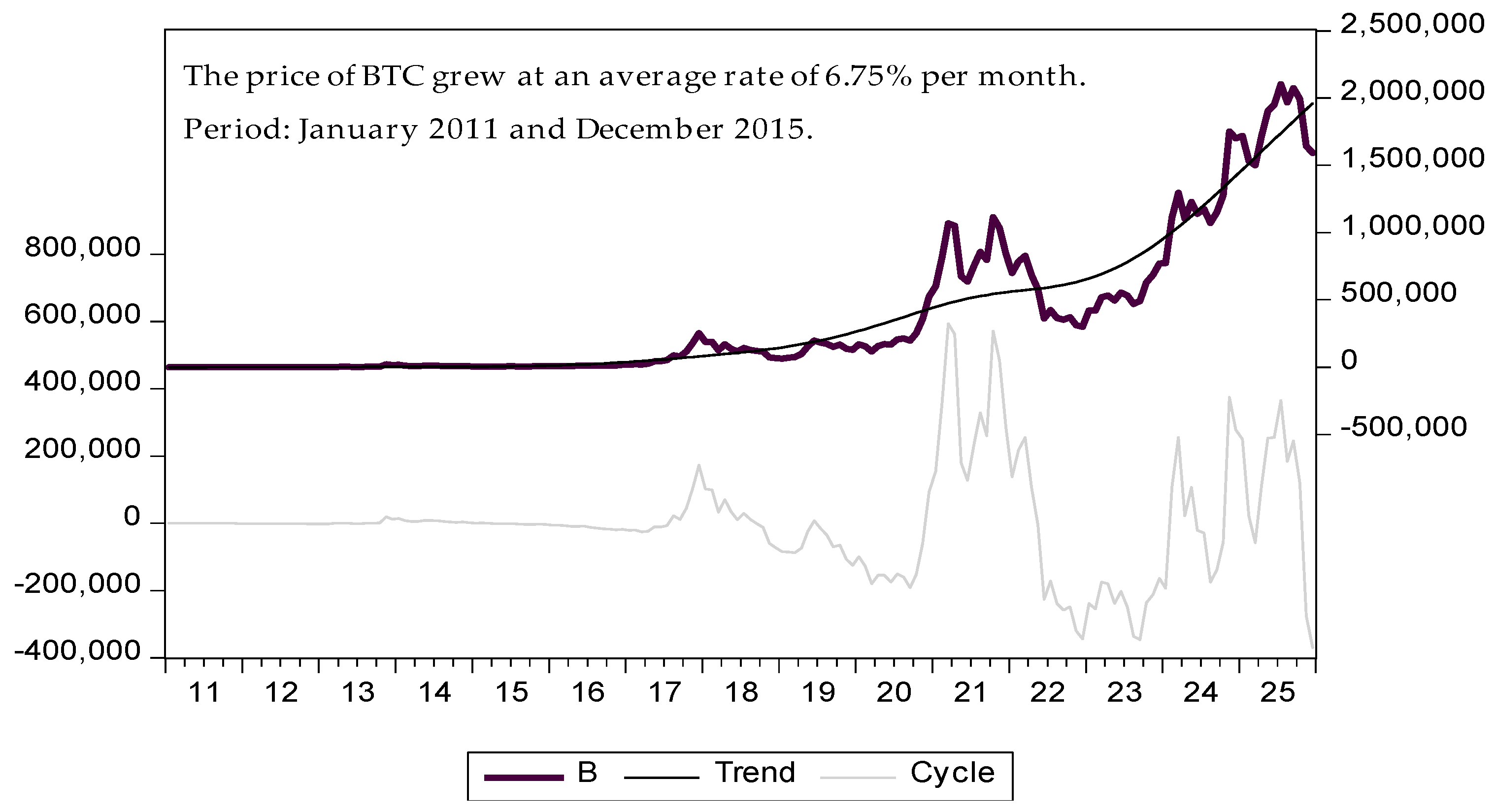
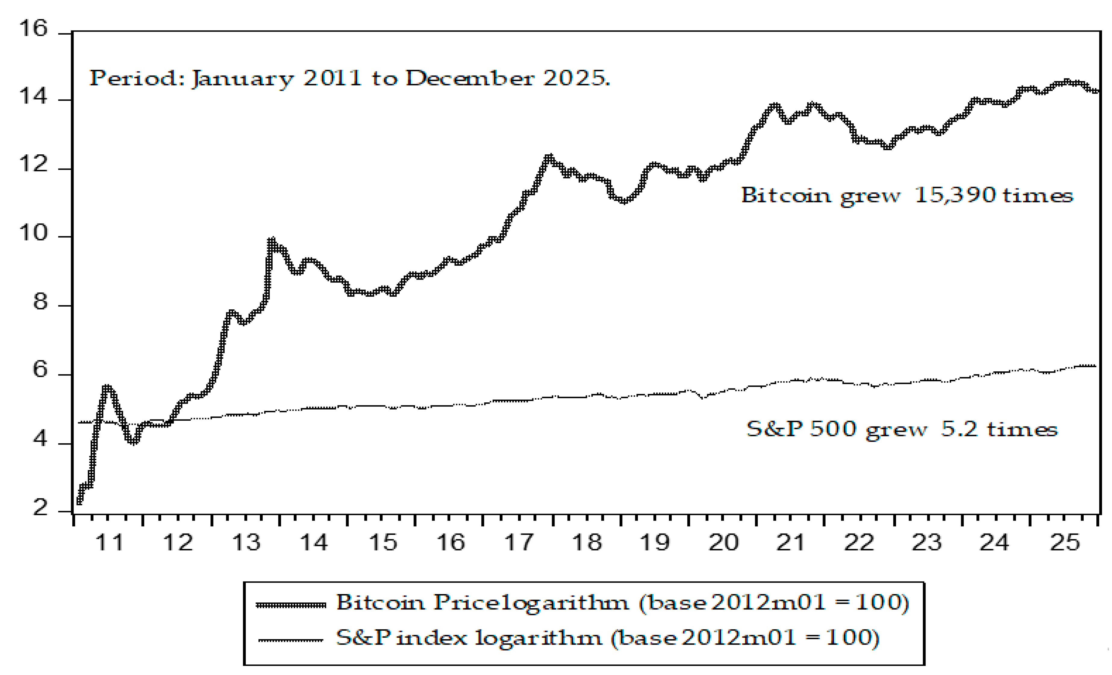
The analysis of stylized facts illustrates the considerable increase in Bitcoin’s profitability during the period 2010–2025. Compared to the Standard & Poor’s 500 index, the difference in performance is significant. While the S&P 500 grew 5.2 times, Bitcoin increased more than 15,930 times. During this period, the average monthly price growth rate remained robust, generating an average annual return of 118.9% and an average monthly return of 6.75%, figures that far exceed those of comparable assets (Appendix A).

Previous research has addressed this topic from different perspectives. First, at the macroeconomic level, a significant relationship has been found between the US Federal Reserve’s monetary policy and Bitcoin prices (returns). Bitcoin is conceived as an online communication protocol that facilitates the use of a virtual currency, including electronic payments (Böhme et al., 2015). Therefore, tightening monetary policy stabilizes the market at low cryptocurrency prices. In scenarios of higher prices, increases in interest rates are associated with a reduction in cryptocurrency prices, and volatility. The findings suggest that changes in interest rates influence the opportunity cost of holding cryptocurrencies, impacting their attractiveness compared to traditional interest-bearing assets (Buthelezi, 2025).

Investors should consider the effects of market-dependent interest rate fluctuations when making Bitcoin-related investment decisions. During periods of low Bitcoin prices, rising interest rates may present opportunities due to their stabilizing effects, while during periods of high prices, investors may need to hedge against potential price declines (Buthelezi, 2025). Another study confirms these findings (Ma et al., 2022), showing that traditional monetary policies significantly influence Bitcoin prices and volatility. However, the impact of monetary policy shocks on Bitcoin may be marginal, meaning low synchronization with it; therefore, it would only be recommended as a hedge in portfolio management. (Elsayed & Sousa, 2024). In contrast to traditional assets, cryptocurrency prices appear to be less affected by macroeconomic factors than the prices of more traditional financial assets. Key drivers of crypto asset prices include market confidence, adoption, technology, and liquidity conditions. Conversely, traditional financial assets are heavily influenced by macroeconomic factors such as interest rates and inflation (Polizu et al., 2023). Empirical results have shown that the impacts of quantitative easing policies on Bitcoin prices can vary over time, with a temporary positive impact observed through different channels. Furthermore, it has been found to exert a long-term positive impact through the liquidity channel (Zhao et al., 2023).

When interest rates rise (restrictive policy), capital migrates to safe-haven assets. Interestingly, when exploring possible explanations for responses to monetary policy shocks in the US, it is found that Bitcoin prices in several emerging market currencies rise particularly sharply after US monetary tightening, especially against the Chinese yuan. Furthermore, based on blockchain transaction data, these currencies systematically flow to exchanges that allow the trading of Bitcoin with emerging market currencies in response to the crisis. The author conjectures that Bitcoin’s technological and institutional characteristics make it resemble a global digital currency that enables cross-border transactions and capital flight (Karau, 2023). However, there is evidence that there have been periods in which interest rates have risen in tandem with increases in Bitcoin prices (Gonzalez et al., 2025).

To date, there is a certain consensus within the scientific community indicating that Bitcoin, linked to blockchain technology, has advantages such as: (i) low transaction costs; (ii) high security, (iii) ease of use, and (iv) real-time settlement (Othman et al., 2020), and that these advantages are affected by the Federal Reserve’s monetary policy.

Second, a significant relationship has been found between the network and the price (return) of Bitcoin. At the microeconomic level, we must understand supply, demand, its value, and the nature of competition (Halaburda et al., 2020). To this end, we emphasize four aspects of the network: (i) The network-value, Metcalfe’s-law literature on active addresses and transactions: Individual addresses capture particular transaction patterns for three regimes, which have evolved as the Bitcoin economy has grown and matured: an initial prototype stage, a second growth stage largely populated by “sinful” enterprises (gambling and black markets), and a third stage marked by a progression from “sinful” companies to legitimate companies (Tasca et al., 2018).

As the number of active addresses increases, so does the price. This growing user base facilitates higher transaction volumes (Koutmos, 2018; Liu et al., 2025). These results provide evidence supporting the long-term impact on the network (Pele & Mazurencu-Marinescu-Pele, 2019; Wheatley et al., 2019), for example, through Metcalfe’s Law, which states that the value of a network is proportional to the square of the number of users connected to the system.

Furthermore, Pele and Mazurencu-Marinescu-Pele (2019) consider a bidirectional causality between price and network size. The expected price increase encourages more investors to join the Bitcoin network, which can lead to super-exponential price growth due to herd behaviour. These results demonstrate the long-term validity of Metcalfe’s Law for cryptocurrency valuation. (Wheatley et al., 2019) also utilize Metcalfe’s Law. Their model captures the universal pattern of the periodic logarithmic power law, which parsimoniously captures various positive feedback phenomena, such as herd behaviour and imitation.

(ii) Cost of Production Valuation: Digital currencies are recognized as an emerging asset class. Not only is there a listed and over-the-counter market for Bitcoin and other digital currencies, but also a booming derivatives market. Therefore, the ability to value Bitcoin and cryptocurrencies becomes fundamental for their consolidation as a legitimate financial asset (Hayes, 2017). Furthermore, he points out that there are three main factors that influence the value of cryptocurrencies: (i) the level of competition in the producer network, (ii) the unit production rate, and (iii) the difficulty of the algorithm used for mining.

The activity of “mining” is carried out by individuals or companies in exchange for the opportunity to obtain Bitcoin blocks. Mining is a necessary component of a cryptocurrency network that is open to the public and does not censor participants from conducting transactions. Mining is performed using specialized hardware that possesses a certain amount of computing power, measured in hashes per second. Hashes can be considered analogous to the processing power of a CPU microchip, which is measured in hertz to define how many individual calculations can be performed per second. The aggregated Bitcoin network has a cumulative computing power that sums all the mining efforts employed worldwide. For every Giga-Hash per second that any individual miner puts online, it is added to the total power of the network (Hayes, 2017, p. 1309).

(iii) Price hash rate causality and endogeneity: The increase in production costs associated with Bitcoin mining shows a negative relationship with prices. This suggests significant potential for reducing the unit cost, reflecting increasing energy efficiency (Fantazzini & Kolodin, 2020). Furthermore, it is considered preferable to treat the hash rate variable directly, rather than using the Cost of Production Model (CPM). It is argued that causality is always unidirectional, from the Bitcoin price to the hash rate, with lags of between one and six weeks, although it reinforces the observed cointegration between the Bitcoin price and the hash rate.

Given that the market has reached greater maturity and regulatory oversight following the introduction of the futures market in 2017, the ban in China and Japan, and considering the recent “Genius Act” (2005), which would have an indirect positive influence on Bitcoin. However, Kubal and Kristoufek (2022), using a system of equations, endogenized the hash rate and discovered that a bidirectional relationship between the hash rate and the price of Bitcoin is possible. They explain that understanding the relationship between the price of Bitcoin and the network’s hash rate is fundamental, as it directly translates into its energy demand and consumption.

(iv) Hedge, safe-haven, and diversifier evidence: There is debate about whether Bitcoin is a reliable investment asset that provides both hedging and portfolio diversification. Studies such as (Bouri et al., 2017a, 2017b; Hougan & Lawant, 2021) move away from hedging, recommending only Bitcoin’s diversification power as a long-term investment asset.

Bouri et al. (2017a, 2017b) demonstrate that Bitcoin constitutes a robust hedge and safe haven against fluctuations in energy commodity indices. Bitcoin’s hedging and safe-haven properties against both raw and energy commodities are only evident in the period leading up to a price drop, while in the period following a drop, Bitcoin is limited to serving as a diversification asset. On the other hand, Bouri et al. (2017a, 2017b) compare the asset as a hedge and safe haven against major global stock market indices, bonds, oil, gold, the overall commodity index, and the US dollar index. The results demonstrate that it is a poor hedge and is only suitable for diversification purposes, which varies depending on the time horizon. In contrast, (Ullah et al., 2024; Urquhart, 2018) indicate that investors are attracted to Bitcoin following significant increases in its volatility and trading volume. Bitcoin also acts as an intraday hedge, diversification tool, and safe haven for certain currencies, which will be of great interest to investors in currencies, cryptocurrencies, and high-frequency trading (Ullah et al., 2024).

This means that Bitcoin improves portfolio diversification, as it is uncorrelated with other assets. More recent studies recommend allocations of 1%, 2.5%, and 5% in asset portfolios for the long term, with favourable results (Hougan & Lawant, 2021). It seems that these studies are generally recommending small allocations that carry little risk and require specific portfolio analysis. However, while these studies present evidence, they do not demonstrate any long-term relationship that can be tested to support not only diversification but also long-term investment in digital assets.

Third, a significant relationship has been found between global volatility and Bitcoin’s price (return). Increased market volatility is expected to negatively impact Bitcoin’s profitability, making it a risky asset. Market sentiment, which fluctuates between fear and euphoria, is systematically linked to Bitcoin’s price. Recent studies support the inclusion of volatility as an explanatory variable for understanding Bitcoin (Jiang & Huang, 2024; Luo et al., 2026; Pogorelova, 2024). Consequently, investors tend to withdraw capital during periods of high volatility, which negatively impacts profitability (Vergili & Celik, 2023). In the context of cryptocurrencies, where price movements are influenced by investor sentiment, sentiment analysis has become a key tool for interpreting market dynamics (Farrugia & Deguara, 2025).

In this context, despite these advances, a significant limitation or problem persists: the lack of research into the long-term relationship between Bitcoin returns and monetary policy, microeconomic variables such as computing power and hash rate, as well as the number of active addresses, and global volatility. Current approaches have not been able to determine whether a cointegration or equilibrium relationship exists in the long term and suggest recommendations for hedging, investing, or diversifying a portfolio. This is due to the lack of extensive data, Bitcoin’s approaching stage of maturity after more volatile initial phases, and the presence of large institutional investors in the cryptocurrency market. This lack of evidence creates gaps that could be addressed.

To address this limitation, this article applies an econometric strategy that employs Autoregressive Distributed Lag (ARDL) models (Pesaran & Shin, 1998; Pesaran et al., 2001). This model examines the relationship between variables within a time series and their respective lags, allowing for the determination of short- and long-term elasticities. Furthermore, a cointegration analysis is performed to assess whether any long-term equilibrium relationship exists between the model’s variables. If so, an Error Correction Model (ECM) will be applied to determine how the explanatory variables in growth rates explain Bitcoin returns. Unlike previous studies, which focus primarily on structural VAR models with two to three endogenous variables, we concentrate on a research problem related to the price (returns) of Bitcoin, using a single equation. This innovative methodology allows us to analyze the phenomenon from the perspective of a dynamic theoretical model.

Based on the previous theoretical review and empirical evidence, we pose the general research question: To what extent do the macroeconomic determinants of US monetary policy (liquidity and the Federal Reserve interest rate), the microeconomic metrics of activity on the blockchain network (users with active addresses and the hash rate), and the volatility of the global market explain price formation (returns) and long-term equilibrium dynamics in the Bitcoin market? In response to this research question, we propose three possible hypotheses (H1, H2, and H3):

H1: 

An expansion of liquidity by the US Federal Reserve raises the price of BTC with a positive long-term elasticity, and the effect of a change in the interest rate materializes with a two-month lag (levels and growth rates).

H2: 

Network activity (active addresses and hash rate) exhibits positive and negative elasticities, respectively, in the long term on the price of BTC (levels and growth rates).

H3: 

An increase in global volatility reduces the price of BTC with a negative elasticity, and its effect is contemporaneous.

The main objective of this research is to analyze the cointegration relationship of the long-term equilibrium between monetary policy factors, microeconomic factors, and global volatility on the price of Bitcoin, from January 2011 to December 2025. The article is structured in four sections, followed by a conclusion. Section 2 details the methodology and defines the econometric model. Section 3 presents the main results, while Section 4 offers a discussion of these findings. Finally, the study concludes with a summary of its contributions and implications.

2. Materials and Methods

2.1. Data

The price of the cryptocurrency BTC and several explanatory variables was used: the interest rate, the FED’s liquidity, the number of active addresses, and the cost of mining or production (blockchain). Since the prices of the selected indices differ significantly from those of other financial assets, logarithmic rates of return were used to calculate the price data, thus preventing excessively large parameter values.

The return series generated for each financial asset uses historical data, where $B_t$ represents the asset price and the logarithmic rate of return was estimated by the model.

Table 1. Summary of variables.

Variable 1	Short Name	Details	Source
Bitcoin price	B	Market Price Bitcoin in USD (BTC).	Investing/COINMARKETCAP
FED—liquidity	L	Total Assets, Millions of USD (WALCL).	The St. Louis Fed data centre (FRED).
Interest rate	R	Federal Reserve Funds Effective Rate (FEDFUNDS).	The St. Louis Fed data centre (FRED)
Active addresses	N	Number of Active Addresses.	CRIPTOQUANT/COINMARKETCAP
Production cost	H	Means Hash Rate.	BLOCKCHAIN
Market volatility	V	CBOE Volatility Index.	Chicago Board Options Exchange (CBOE)/FRED

¹ Monthly variables have a base year of January 2012 = 100, except for the interest rate. The Fed Interest Rate is the only variable entering the model without transformations. Source: Authors with own compilation extracted from sources. The dataset of File S1 is available in the online repository: https://doi.org/10.7910/DVN/U4XPQM.

presents the details of each variable according to its source. We have five (5) explanatory variables with data from the period January 2011 to December 2025, with 180 monthly observations per variable.

2.2. Method

The theoretical framework posits a mathematical model underpinned by variables identified throughout the literature review and supported by empirical evidence concerning the determinants of Bitcoin (BTC) pricing. It is hypothesized that BTC price fluctuations are driven by factors such as the Federal Reserve’s monetary policy instruments, microeconomic metrics inherent to the Bitcoin network, and broader environmental variables—specifically market volatility as represented by the VIX. The functional relationship, incorporating the operational variables, is expressed in Equation (1) as follows:

$$B_t=f(L_t,R_t,N_t,H_t,V_t)$$

(1)

where

• $B_t$: The natural logarithm of the Bitcoin (BTC) market price, denominated in US Dollars.
• $L_t$: The natural logarithm of the Federal Reserve’s Total Assets (expressed in millions of US Dollars), serving as a proxy for liquidity.
• $R_t$: The Federal Funds Effective Rate, expressed in decimal form.
• $N_t$: The natural logarithm of the number of active addresses within the network.
• $H_t$: The natural logarithm of the mean Hash Rate, representing the network’s computational power.
• $V_t$: The CBOE Volatility Index (VIX), utilized as a measure of broader market risk and investor sentiment.

Equation (1) defines the empirical specification for the BTC price variable. Consequently, the primary model under consideration is formulated in Equation (2) as follows:

$$\ln \left(B_t\right)={\beta }_0+{\beta }_1\ln \left({\mathrm{L}}_{\mathrm{t}}\right)+{\beta }_2\ln \left({\mathrm{R}}_{\mathrm{t}}\right)+{\beta }_3\mathrm{l}\mathrm{n}\left({\mathrm{N}}_{\mathrm{t}}\right)+{\beta }_4\ln \left({\mathrm{H}}_{\mathrm{t}}\right)+{\beta }_5\ln \left({\mathrm{V}}_{\mathrm{t}}\right)+{\epsilon }_t$$

(2)

Autoregressive Distributed Lag (ARDL) econometric models are linear specifications designed for time-series analysis, wherein dependent and independent variables are related both contemporaneously and through their respective lagged values (Narayan, 2004, 2005; Pesaran & Shin, 1998; Pesaran et al., 2001). The general ARDL (p, q₁, q₂, q₃, …, q_k) framework facilitates the estimation of growth rates (denoted in lowercase) for the Bitcoin price variable, represented here by the endogenous variable $B_t$, an endogenous variable. The corresponding exogenous variables—$L,R,N,H$, and V—are detailed in Table 1 and expressed in simplified form in Equation (3).

$$B_t={\alpha }_0+{\alpha }_{1}t+{\mathsf{\delta }D}_{2018,t}+{\displaystyle {\sum }_{i=1}^p}{\psi }_i{B}_{t-i}+{\displaystyle {\sum }_{j=1}^k}\ast {\displaystyle {\sum }_{l_j=0}^{q_j}}{\beta }_{j,l_j}{X}_{j,t-lj}+{\epsilon }_t$$

(3)

where ε_t represents innovations, α₀ is a constant term, α₁ is the coefficient associated with a linear trend, $D_{2018,12}$ is the dummy step variable (0) before December 2017 and (1) after $\delta$ captures the permanent shift in the level of ($B_t$) after the regulatory shock.

ψ_i is the coefficient associated with lags of B_t, and β_j,lj are the coefficients associated with lags of k regressors X_t,j for j = 1, 2, 3, …, k.

The initial stage of the ARDL application involves the estimation of intertemporal dynamics. These models were estimated using Ordinary Least Squares (OLS), whereby the endogenous variable was regressed on a set of exogenous factors and their respective lags. Empirical evidence shows that the optimal lag structure was subsequently determined by selecting the specification that minimizes the Akaike Information Criterion (AIC), ensuring a parsimonious balance between model fit and complexity (Gonzales & Varona, 2023; Varona & Gonzales, 2025; Varona et al., 2024).

A bounds testing procedure was employed to ascertain the existence of a long-run relationship, thereby facilitating the derivation of the Error Correction Model (ECM) to capture short-run dynamics. The F-test was conducted under the null hypothesis of no cointegration among the variables. The resulting test statistic is compared against two asymptotic critical value bounds, corresponding to cases where the regressors are purely ($H_0$), purely ($H_1$), or mutually cointegrated. If the calculated F-statistic exceeds the upper critical bound, the null hypothesis ($H_0$) is rejected, confirming a stable long-run equilibrium.

In the presence of cointegration, the short-run elasticities can also be derived by an Error Correction Model (ECM) in Equation (4) as follows:

$$\begin{gathered} ∆ln{\left(B\right)}_t={\beta }_0+{\displaystyle \sum _{i=1}^p}{\beta }_1∆ln{\left(B\right)}_{t-i}+{\displaystyle \sum _{i=0}^{q1}}{\beta }_2∆ln{\left(L\right)}_{t-i}+{\displaystyle \sum _{i=0}^{q2}}{\beta }_3∆\ln {\left(X\right)}_{t-i} \\ +\psi {\left(ECT\right)}_{t-1}+{\mathsf{\delta }D}_{2018,12}+{\vartheta }_t \end{gathered}$$

(4)

ECT_t−1 is the error correction term. Δ is the first difference operator. β’s are the coefficients related to the short-term dynamics of the convergence-to-equilibrium model. ψ is the measure of the speed of adjustment. X represents other variables such as the US Federal Reserve interest rate, active addresses, the hash ratio, and global volatility (VIX index). Additionally, we include the variable D_2018,12, which represents a dummy variable for “structural breakdown”, through the stability analysis of the parameters (Brown et al., 1975; Chow, 1960; Zivot & Andrews, 1992).

Short-run analysis found a long-run cointegration relationship between the exogenous variables and the endogenous variable. The long-run relationship was tested. An F-test was used with the null hypothesis that the variables are not cointegrated. The test statistic was computed and compared to two asymptotic critical values corresponding to cases where the variables are I(0) or I(1). When the test statistic is above the critical value, the null hypothesis is rejected and the conclusion is that cointegration is possible, and an ECM can be estimated.

3. Results

3.1. Unit Root and Stationarity Tests

The results indicate that the variables are stationary in their first differences, except ln(V), which is stationary in levels; that is, we have variables I(0) and I(1). To analyze the stochastic properties of the Data and determine the order of integration of the variables, we employ the Augmented Dickey–Fuller (ADF) and Phillips–Perron (PP) unit root tests, complemented by the Kwiatkowski–Phillips–Schmidt–Shin (KPSS) stationarity test (Appendix B).

The empirical evidence indicates that the series ln(B), ln(L), R, ln(N), and ln(H) are non-stationary in levels. For these variables, the ADF and PP test statistics fail to reject the null hypothesis of a unit root at conventional significance levels, while the KPSS test rejects the null of stationarity. Conversely, upon transforming the data into first differences, the null of a unit root is rejected at the 1% level across all specifications, confirming that these processes are integrated of order one, I(1). In contrast, the variable ln(V) exhibits stationarity in levels. The ADF and PP statistics for ln(V) are significant at the 1% level (p < 0.01), and the KPSS test fails to reject the null of stationarity, identifying the series as I(0). Given the presence of a mixture of I(1) and I(0) processes, the Autoregressive Distributed Lag (ARDL) bounds testing approach is favoured for the subsequent cointegration analysis, as it remains consistent regardless of the underlying order of integration, provided no variable is I(2).

3.2. ARDL Bound Tests for Cointegration

Table 2. Cointegration with bound test. Pesaran et al. (2001) vs. Narayan (2005).

Model	k (n)	F-Stat	Pesaran et al. (2001) Asymptotic [I(0)–I(1)]	Narayan (2005) Finite Sample [I(0)–I(1)]	Cointegration (5%)	Method
1	5 (179)	3.96	[2.39–3.38]	[2.55–3.61]	Yes	ECM
2	5 (179)	3.52	[2.39–3.38]	[2.55–3.61]	Inconclusive	∆ (ARDL)
3	5 (179)	3.53	[2.39–3.38]	[2.55–3.61]	Inconclusive	∆ (ARDL)
4	4 (168)	3.87	[2.56–3.49]	[2.68–3.69]	Yes	ECM

Note: Model 1 specifies Equation (2) with a single lag. Model 2 incorporates dummy variables and two lags for diagnostic correction. Model 3 extends the structure to three lags. Model 4 employs the AIC (max 12 lags).

presents the results of the bounds testing procedure for cointegration. The empirical evidence confirms the existence of a long-run cointegrating relationship across both proposed models, significant at the 5% level (Model 1 and Model 4). The calculated F-statistics were benchmarked against the asymptotic critical values of (Pesaran et al., 2001) and the finite-sample adjusted bounds of (Narayan, 2005). The empirical evidence confirms a robust long-run equilibrium relationship for Models 1 (F = 3.96) and 4 (F = 3.87), as both statistics exceed the (Narayan, 2005) upper I(1) bound at the 5% significance level (3.61 and 3.69, respectively).

Regarding Models 2 and 3, the test statistics fall within the inconclusive zone under the finite-sample criteria at the 5% level. Consequently, adopting a conservative econometric stance, we proceed with the Error Correction Model (ECM) estimation exclusively for those specifications exhibiting robust cointegration (Models 1 and 4). For Models 2 and 3, the analysis focuses solely on short-run dynamics via first-differenced variables, which are omitted here for brevity.

Table 3. Cointegration with bound test. Model estimates with structural change in 2018:M12.

Model	k (n)	F-Stat	Pesaran et al. (2001) Asymptotic [I(0)–I(1)]	Narayan (2005) Finite Sample [I(0)–I(1)]	Cointegration (5% and 1%)	Method
1	5 (179)	4.487	[2.39–3.38]	[2.55–3.61]	Yes **	ECM
2	5 (179)	3.945	[2.39–3.38]	[2.55–3.61]	Yes **	ECM
3	5 (179)	3.915	[2.39–3.38]	[2.55–3.61]	Yes **	ECM
4	4 (168)	8.706	[3.29–4.37]	[3.602–4.787]	Yes ***	ECM

Note: *** and ** indicate statistical significance at the 1% and 5% levels, respectively.

considers a structural disruption variable that improves upon the results of Table 2, as can be seen, with model 4 being statistically significant at the 1% level and the others at the 5% level. This takes into account the regulatory change in cryptocurrencies for a market that held more than 25% of the total. In 2017, China banned cryptocurrency funding and ICOs and closed cryptocurrency exchanges (Xie, 2019). While the United States recognizes certain cryptocurrencies as functional equivalents of fiat currencies, China explicitly, though only nominally, delegitimizes this function to preserve its regulatory strength in capital controls. The United States adopted a flexible approach and regulated their use. It recognizes Bitcoin as a functional substitute for real currency (Xie, 2019).

Then, using graphical analysis of the Bitcoin logarithm (LB), a possible structural break point is observed, defining two stages of evolution for the period 2011m01 to 2025m12. This event would be associated with the regulation of Bitcoin in major economies such as the US and China (Peetz & Mall, 2019; Xie, 2019), following accusations of fraud and money laundering (Chainalysis, 2022; Kerr et al., 2023). In addition, (Chow, 1960) and (Zivot & Andrews, 1992) were applied to confirm a dummy variable for the structural break, capturing a regulatory change for 2018m12.

The re-estimated ARDL bound test results, incorporating a structural break adjustment, provide compelling evidence of long-run equilibrium relationships across all specifications. As detailed in Table 3, the calculated F-statistics for Models 1, 2, and 3 (ranging from 3.9157 to 4.487) comfortably exceed the 5% finite-sample upper bound of 3.61 established by (Narayan, 2005).

Furthermore, Model 4 exhibits remarkable robustness with an F-statistic of 8.706, surpassing the 1% significance threshold of 4.787. The consistent rejection of the null hypothesis of no cointegration across all models validates the transition to the Error Correction Model (ECM) framework. This allows for a precise estimation of the speed of adjustment and the long-run elasticities between Bitcoin price, network fundamentals (“blockchain”), and macro-financial determinants.

3.3. Causality and Endogeneity Considerations (Granger Tests)

To address potential endogeneity and ascertain the directional dynamics of the system, Granger causality tests were performed in both levels (Appendix C,

Table A3. Granger causality tests (Lags 1 and 2), level.

Null Hypothesis	Lag 1	Lag 2	Decision (α = 0.05)
LL does not Granger Cause LB	0.54	0.46	Fail to Reject
LB does not Granger Cause LL	0.80	0.25	Fail to Reject
R does not Granger Cause LB	0.28	0.36	Fail to Reject
LB does not Granger Cause R	0.29	0.37	Fail to Reject
LN does not Granger Cause LB	0.65	0.88	Fail to Reject
LB does not Granger Cause LN	0.36	0.00 *	Reject Null (only Lag 2)
LH does not Granger Cause LB	0.81	0.51	Fail to Reject
LB does not Granger Cause LH	0.00 *	0.00 *	Reject Null (Robust)
LVIX does not Granger Cause LB	0.47	0.97	Fail to Reject
LB does not Granger Cause LVIX	0.57	0.21	Fail to Reject

Note: * Significant at the 1% level.

) and first differences (Appendix C,

Table A4. Granger causality tests (Lags 1 and 2), first difference.

Null Hypothesis	Lag 1	Lag 2	Decision (α = 0.05)
D(LL) does not Granger D(LB)	0.24	0.34	Fail to Reject
D(LB) does not Granger D(LL)	0.41	0.38	Fail to Reject
D(R) does not Granger D(LB)	0.28	0.33	Fail to Reject
D(LB) does not Granger D(R)	0.58	0.18	Fail to Reject
D(LN) does not Granger D(LB)	0.29	0.59	Fail to Reject
D(LB) does not Granger D(LN)	0.00 *	0.00 *	Reject Null
D(LH) does not Granger D(LB)	0.85	0.54	Fail to Reject
D(LB) does not Granger D(LH)	0.00 *	0.00 *	Reject Null
D(LVIX) does not Granger D(LB)	0.84	0.96	Fail to Reject
D(LB) does not Granger D(LVIX)	0.32	0.02 *	Reject Null (only Lag 2)

Note: * Significant at the 5% level or better. The results report Granger causality tests for Lags 1 and 2. Additionally, tests are conducted up to Lag 12 (for both levels and first differences). While intermittent bidirectional significance is detected at higher-order lags (specifically months 6, 8, and 10) for Active Addresses (LN), Hash Rate (LH), and the VIX, these relationships are considered weak and lag-dependent. The primary short-run dynamic remains a unidirectional flow from Bitcoin price (LB) to network fundamentals (LN, LH, and LV).

). This analysis is critical to validating the research framework and responding to potential feedback loops between the Bitcoin price (LB), intrinsic network variables, and the macro-financial environment.

The empirical results reveal a clear and persistent distinction regarding the role of the determinants: (i) Macro-financial Factors and Market Volatility (LL, R, and LVIX): The Granger tests find no evidence of unidirectional causality running from global liquidity (LL), the interest rate (R), or the VIX volatility index (LVIX) towards the Bitcoin price, across both levels and differences. Specifically regarding the VIX, the absence of short-run causality suggests that Bitcoin does not react mechanically or instantaneously to global market fear; rather, it shares a long-run equilibrium nexus with financial stability. Notably, in the first-difference specification (Appendix C, Table A4), the Bitcoin price shows signs of preceding the VIX at the second lag, suggesting a delayed interconnection with traditional market volatility.

(ii) Internal Network Variables (LN, and LH): Conversely, there is robust unidirectional Granger causality (p < 0.01) running from the Bitcoin price to the Hash rate (LH) and Active Addresses (LN). In levels (Appendix C, Table A3), this relationship is particularly evident for the Hash Rate from the first lag, whilst for active addresses, it manifests at the second lag. These findings confirm that network fundamentals are endogenous to price movements; price discovery acts as the primary catalyst incentivising mining power and user adoption, aligning with the existing literature (Fantazzini & Kolodin, 2020).

Collectively, the absence of causality running from the regressors to the price across all specifications reinforces the suitability of the ARDL bound-testing framework. As there is no clear directional causality “driving” Bitcoin from the macro-financial environment or network fundamentals in the short run, the results are interpreted as a “stochastic equilibrium association” where the Bitcoin price co-evolves synchronously with the global financial system and its own technical infrastructure through a complex feedback ecosystem.

Whilst we acknowledge that the (Toda & Yamamoto, 1995) procedure is a robust alternative for testing Granger causality in the presence of mixed integration orders, it is primarily situated within a VAR framework. In this study, we deliberately prioritize the ARDL bound-testing approach due to its documented superior performance in finite samples (Narayan, 2005) and its efficiency in capturing the long-run equilibrium vector without the over-parameterization risks associated with VAR-based causality tests. Furthermore, the standard Granger tests performed in this study consistently yield results aligned with the literature, within the scope of our equilibrium-focused analysis.

3.4. ARDL Estimation

Table 4. ARDL model.

Model	(1)	(2)	(3)	(4)
LB(−1)	0.96 ***	0.95 ***	0.96 ***	0.89 ***
LL	2.01 ***	2.47 ***	2.48 ***	0.28 ***
LL(−1)	−1.87 ***	−2.35 ***	−2.35 ***	---
R	0.02	0.02	0.02	−0.01
R(−1)	---	---	---	−0.24
R(−2)	---	---	---	0.61 **
R(−3)	---	---	---	−0.53 *
R(−4)	---	---	---	0.51
R(−5)	---	---	---	−0.30
R(−6)	---	---	---	0.09
R(−7)	---	---	---	−0.18
R(−8)	---	---	---	0.01
R(−9)	---	---	---	−0.04
R(−10)	---	---	---	0.29
R(−11)	---	---	---	−0.53 *
R(−12)	---	---	---	0.44 ***
LN	0.93 ***	0.93 ***	0.93 ***	0.83 ***
LN(−1)	−0.82 ***	−0.82 ***	−0.82 ***	−0.52 ***
LN(−2)	---			−0.09
LN(−3)	---			0.13
LN(−4)	---			−0.20
LN(−5)	---			0.002
LN(−6)	---			0.36 ***
LH	−0.26 ***	−0.26 ***	−0.26 ***	−0.08
LH(−1)	0.23 ***	0.23 ***	0.23 ***	0.10
LH(−2)	---	---	---	−0.28
LV	−0.32 ***	−0.30 ***	−0.29 ***	−0.16 **
Constant	0.01	0.06	0.07	−3.54 ***
D1: January 2020	---	0.02	0.02	---
D2: January 2022	---	−0.09	−0.10	---
D3: November 2022	---	−0.14	−0.15	---
D4: December 2022	---	−0.01	0.01	---
D5: December 2024	---	0.15	---	---
D6: December 2018	0.17 **	0.18 **	0.18 **	0.25 ***
R2 Adjust	0.9942	0.9942	0.9942	0.9951
F-statistic	2889 ***	1895 ***	2033 ***	1057 ***
AIC	0.05	0.09	0.08	−0.17
Jarque–Bera	0.00 < 0.05	0.00 < 0.05	0.00 < 0.05	0.00 < 0.05
LM test (1rez)	0.80 > 0.05	0.93 > 0.05	0.85 > 0.05	0.051 > 0.05
ARCH test	0.20 > 0.05	0.20 > 0.05	0.20 > 0.05	0.16 > 0.05
Ramsey test	0.28 > 0.05	0.37 > 0.05	0.33 > 0.05	0.08 > 0.05
CUSUM Test (ST)	no	yes	yes	yes

Note: ***, ** and * indicate statistical significance at the 1%, 5%, and 10% levels, respectively.

presents the estimation results for the ARDL framework. In Model 1, the findings provide evidence of a positive relationship between liquidity and the BTC price, yielding a coefficient of +2.01, which is statistically significant at the 1% level. Conversely, the Federal Reserve’s interest rate exhibits a direct relationship with a coefficient of 0.02, although it is not statistically significant. Furthermore, both the proliferation of active addresses and the marginal cost of mining are significant at the 1% level, with coefficients of +0.93 and −0.26, respectively. The VIX volatility index confirms an inverse relationship with the BTC price (coefficient of −0.32, significant at the 1% level). The structural breakdown dummy variable is statistically significant at the 1% level with a coefficient of +0.17. Consequently, Model 2 was estimated, which incorporates dummy variables to account for specific periods of high BTC volatility, facilitating the CUSUM test, the COVID-19 pandemic, and the December 2018 dummy variable due to the structural change. This modification improves both the results and the parametric stability tests.

In Model 3, the lag structure was extended (3 lags). The impact of liquidity reflects a marginal improvement, yielding a coefficient of 2.48, which remains statistically significant at the 1% level. It should be noted that the current Federal Reserve interest rate appears to be weakening, with a coefficient of 0.02 (but not significant at the 33% level). Overall, this specification does not yield substantial departures from the previous models.

Model 4 is extended to a lag of 12 periods using the Akaike Information Criterion (AIC). In this context, contemporaneous liquidity remains stable with a coefficient of +0.28, statistically significant at the 1% level. Additionally, the results indicate that the interest rate, after a two-period lag (equivalent to approximately 90 days), has a coefficient of +0.61, statistically significant at the 5% level. Moreover, until period 12, a coefficient of +0.44 is observed, which is statistically significant at the 1% level.

In addition, the proliferation of active addresses maintains a statistically significant coefficient of +0.83 (significant at the 1% level), and its influence extends to lag 6 with a coefficient of +0.36, statistically significant at the 1% level. The VIX volatility index continues to exhibit an inverse relationship with the BTC price, yielding a coefficient of −0.16, significant at the 5% level. Notably, Model 4 satisfies the requisite diagnostic and parametric stability tests—specifically the CUSUM test (except for Model 1).

Model 4 serves as a robust sensitivity analysis, given that the Akaike Information Criterion (AIC) is less parsimonious than the Schwarz Criterion in its selection of lags. Despite variations in magnitude, the signs associated with the monetary policy variables remain consistent across all specifications, with liquidity coefficients of +2.01, +2.47, +2.48, and +0.28 for Models 1 through 4, respectively (statistical significance of 1%). The interest rate demonstrates a positive impact in the second lag (coefficient of +0.61). The AIC framework thus facilitates the identification of lagged transmission effects that the Schwarz Criterion might overlook. Specifically, the AIC results suggest that while Federal Reserve liquidity exerts an immediate impact in the current month, the influence of interest rate adjustments only materializes in the second month, and then in month 12, providing a more nuanced understanding of monetary policy dynamics.

The AIC specification functions as a robustness test; the inclusion of twelve lags confirms that, while Bitcoin exhibits marked short-term volatility, long-term equilibrium (cointegration) remains robust. Consequently, both the bound test and the F-statistic validate the collective explanatory power of the variables. The results confirm that Bitcoin cointegrates with the selected determinants, as demonstrated by the F-statistics (2889, 1895, 2033, and 1057), which are statistically significant at the 1% level.

The formal selection of the optimal structural specification uniquely points to Model 4. The statistical decision rule employed for this selection is the Akaike Information Criterion (AIC), whereby the most negative value determines the optimum fit. In terms of the ARDL levels, Model 4 formally minimizes this criterion by yielding the lowest Akaike value (−0.17 < 0.05 < 0.08 < 0.09), thereby confirming the statistical superiority of this specification. The transition from Models (1–3) to the optimal twelve-lag structure (Model 4) induces substantial shifts in the estimated parameters; most notably, the contemporaneous coefficient of liquidity undergoes a sharp reduction from average values above two (+2.01, +2.47, and +2.48) to stabilize at (+0.28), whilst the hash rate ratio loses statistical significance, moving from (−0.26) to (−0.08).

This dynamic is underpinned by three complementary econometric foundations: (i) the initial truncated specifications suffered from omitted-lag bias, which forced contemporaneous coefficients to artificially absorb the temporal persistence and unexplained inertia, (ii) extending the structure to twelve lags captures the full temporal dynamics of the monthly frequency series, effectively purging the residuals of autocorrelation, and (iii) treating the VIX as a contemporaneous, fixed factor aligns with its integration of order zero, I(0), as validated by unit root and stationarity analysis. Enforcing a lagged structure on a mean-reverting, stationary global exogenous variable would introduce severe over-parameterization and multicollinearity, thereby distorting the net marginal impact of the remaining determinants.

The ARDL model was successfully evaluated against the fundamental Gauss–Markov assumptions, meeting the criteria for linearity, homoscedasticity, and the absence of perfect multicollinearity among the explanatory variables (liquidity, interest rates, active addresses, hash rate, and VIX). However, the Jarque–Bera (JB) test strongly rejects the null hypothesis of normally distributed residuals (JB = 0.00, p < 0.05).

This violation of the normality assumption does not invalidate the model; rather, it aligns directly with the established stylized facts of high-frequency and highly volatile financial time series (Abdullaev & Ibragimov, 2026; Chu et al., 2015; Katsiampa, 2017). As documented extensively in the digital asset literature, cryptocurrency asset returns typically exhibit heavy-tailed distributions and significant skewness due to sudden market shocks, liquidations, and behavioural shifts. Given that the sample size is large (N = 180), we invoke the Central Limit Theorem (CLT). Asymptotically, the OLS estimators remain unbiased, consistent, and valid for statistical inference and hypothesis testing, even in the absence of normally distributed error terms.

3.5. Error Correction Model Estimation

Once cointegration was identified, the Error Correction Model (ECM) was estimated, the results of which are presented in

Table 5. EC model.

Model	(5)	(6)	(7)	(8)
Long-run coefficient
LL	3.78	2.84	2.94	2.67 ***
	(3.20)	(2.65)	(2.79)	(0.94)
R	0.41	0.38	0.38	0.83 ***
	(0.49)	(0.42)	(0.44)	(0.25)
LN	2.83	2.60	2.69	4.76 ***
	(2.49)	(2.06)	(2.20)	(1.45)
LH	−0.74	−0.59	−0.62	−0.90 ***
	(0.88)	(0.69)	(0.74)	(0.38)
LV	−8.49	−6.88	−7.17	---
	(6.26)	(4.65)	(5.01)	---
C	0.25	1.51	1.68	−33.18 ***
	25.94)	(23.07)	(24.09)	(11.31)
Short-run coefficient
ECM(−1)	−0.0377 ***	−0.0436 ***	−0.0418 ***	−0.1067 ***
dll	2.01 ***	2.47 ***	2.48 ***	---
dr	---	---	---	−0.01
dr(−1)	---	---	---	−0.35 **
dr(−2)	---	---	---	0.26
dr(−3)	---	---	---	−0.27
dr(−4)	---	---	---	0.23
dr(−5)	---	---	---	−0.06
dr(−6)	---	---	---	0.03
dr(−7)	---	---	---	−0.14
dr(−8)	---	---	---	−0.15
dr(−9)	---	---	---	−0.20
dr(−10)	---	---	---	0.09
dr(−11)	---	---	---	−0.44 ***
dln	0.93 ***	0.93 ***	0.93 ***	0.83 ***
dln(−1)	---	---	---	−0.19
dln(−2)	---	---	---	−0.29 **
dln(−3)	---	---	---	−0.15
dln(−4)	---	---	---	−0.37 ***
dln(−5)	---	---	---	−0.36 ***
dlh	−0.26 ***	−0.26 ***	−0.26 ***	0.08
dlh(−1)	---	---	---	0.28 1
lv	---	---	---	−0.10 ***
D1: 2020.01	---	0,01	0.01	---
D2: 2022.01	---	−0,09	−0.10	---
D3: 2022.11	---	0,01	0.01	---
D4: 2022.12	---	−0,14	−0.15	---
D5: 2024.12	---	0.15
D6: 2018.12	0.17 ***	0.18 ***	0.18 ***	0.25 ***
R2	0.35	0.36	0.36	0.44
AIC	−0.014	0.027	0.021	−0.228

Note: ***, ** and * indicate statistical significance at the 1%, 5%, and 10% levels, respectively. ¹ Indicates statistical significance at 12%.

. In the long run, none of these three models yield statistically significant results; therefore, no conclusions can be drawn regarding the coefficients. However, Model 8 is the unique specification that presents significant coefficients for liquidity (+2.67), the US Federal Reserve interest rate (+0.83), active addresses (+4.76), and the hash rate (−0.90), all at the 1% significance level. This confirms that Federal Reserve monetary policy (liquidity and interest rates) maintains a long-run equilibrium relationship with the price of Bitcoin, alongside the microeconomic variables associated with the Bitcoin network (blockchain). Whenever deviations from equilibrium occur, adjustments take place to restore a robust cointegrating relationship in pursuit of long-run equilibrium.

In the short run, empirical evidence supports the hypothesis of a positive relationship between the liquidity growth rate, with a coefficient of +2.01, and BTC returns. Furthermore, the number of active addresses and the BTC production cost are statistically significant at the 1% level, with coefficients of +0.93 and −0.26, respectively (Model 5). Models 6 and 7 display similar results. In Model 8, the growth rate of the interest rate lagged by one period (−0.35) becomes statistically significant at the 5% level and remains so up to the 11th lag, with a coefficient of −0.44 significant at the 1% level. Additionally, the contemporaneous number of active addresses is statistically significant at the 1% level with a coefficient of +0.83, exerting an influence up to the 5th lag with a coefficient of −0.36, which is significant at the 1% level. Regarding the hash rate, evidence of statistical significance was found at the 12% level, reinforcing the notion of a potential bidirectional relationship.

Subsequently, market volatility exhibits a negative contemporaneous impact on BTC returns, with a coefficient of −0.10 significant at the 1% level. The structural break dummy variable for December 2018 confirms a positive and statistically significant relationship at the 1% level.

According to the empirical evidence obtained, we chose Model 4 (in levels) and Model 8 (in growth rates), which show a robust relationship in levels and growth rates between the variables, confirming how monetary policy affects the price of Bitcoin, showing how microeconomic variables explain its price and how in the environment, volatility has a negative behaviour.

In the Error Correction Model (ECM), the best model for growth rates, based on the Akaike Criterion and Information, is Model 8 (−0.228 < −0.014 < 0.021 < 0.027). It can be seen that the long-term elasticities are more stable than those presented in the short term and are statistically significant at the 1%. Table 5 shows that, in all the models presented, the error coefficient variable, ECM (−1), meets the three necessary conditions: it has a negative sign, a value less than one, and is statistically significant. In Model 8, the model variables cointegrate until they reach long-term equilibrium and, in the short run, are corrected with an adjustment rate toward equilibrium of 10.67%. That is, for the variables to fully return to their long-term equilibrium relationship, the system will take approximately 9.4 months.

4. Discussion

There is empirical evidence supporting the hypothesis that the Federal Reserve’s (FED) liquidity expansion has a long-term positive impact on the price of Bitcoin. This evidence has a coefficient of 2.67, statistically significant at the 1% level.

Quantitative easing has a direct upward effect on the price of Bitcoin. The underlying transmission mechanism suggests that as the Fed injects capital into the financial system, this cheap money flows into the stock and cryptocurrency markets, a phenomenon clearly observed globally following the onset of the COVID-19 pandemic and subsequent government stimulus measures. Previous research (Buthelezi, 2025; Sadraoui et al., 2021; Tosun & Uğurlu, 2025) has found that Bitcoin has a long-term relationship with and reacts to changes in monetary policy, and that its impact persists beyond the second month after implementation.

Furthermore, the data corroborate the role or transmission mechanism of liquidity in driving long-term prices (Zhao et al., 2023). An alternative perspective suggests that Bitcoin appreciates as investors seek a hedge against fiat currency devaluation in a context of high economic activity and general optimism (Srinivasan et al., 2022). Consequently, Bitcoin could be considered not only a speculative asset but also a viable hedge against inflation. A deep understanding of these liquidity cycles is essential for developing conservative portfolio management and sound funding strategies (Smales, 2020).

In the long term, there is empirical evidence supporting the hypothesis that the Federal Reserve’s benchmark interest rate has a positive long-term impact on the price of Bitcoin, with a coefficient of 0.83 (statistically significant at the 1% level). In the short term, the results show that adjustments to interest rate growth (lags 1 and 11, with statistical significance at 5% and 1%, respectively) would have a negative impact. This suggests a direct relationship between the Federal Reserve’s interest rate policy and the price of Bitcoin. While the existing literature identifies correlations between Bitcoin and macroeconomic variables (Farrugia & Deguara, 2025; Polizu et al., 2023), few studies employ dynamic ARDL econometric models to isolate the specific impact of monetary policy through interest rates and liquidity controls. The positive relationship observed here suggests that rising interest rates often coincide with economic booms, which generally boost demand for risk assets (Havidz et al., 2021; Köse et al., 2026; Kumar & Ajaz, 2022).

Collectively, liquidity and interest rates create a pro-cyclical “virtuous cycle” for Bitcoin’s growth. An expansion of the money supply facilitates capital inflows into alternative assets; at the same time, Bitcoin demonstrates resilience to higher interest rates when ac-companied by a strong economy and inflationary pressures against which investors seek protection. Therefore, market participants are advised to closely monitor Federal Reserve guidance when formulating investment strategies or managing portfolios.

In the long run, active addresses have a positive impact with a statistically significant coefficient of +4.76 at the 1% level. In contrast, this is adjusted in the short run, with a coefficient of +0.83 (contemporary), reaching statistical significance at the 1% level in model 4. The prevailing trend indicates that as the number of active addresses increases, so does the price. This growing user base facilitates higher transaction volumes, consistent with the strong correlations identified in the existing literature (Koutmos, 2018; Liu et al., 2025). Furthermore, in accordance with the law of demand, Bitcoin’s valuation is positively influenced by the volume of transactions within its evolving market microstructure, leading to long-term price increases.

These results provide evidence supporting Metcalfe’s Law in the long run. In the short run, the variable has three negative coefficients: lag (2), lag (4), and lag (5), with coefficients of −0.29, −0.37, and −0.36, respectively, all statistically significant at the 5% level. This is because there is ample evidence of its long-term impact on the network (Pele & Mazurencu-Marinescu-Pele, 2019; Wheatley et al., 2019), for instance, through Metcalfe’s Law, which states that the value of a network is proportional to the square of the number of users connected to the system.

In the long term, the hash rate has a negative impact with a coefficient of −0.90, statistically significant at the 1% level. In contrast, in the short term, with a coefficient of +0.28 (lagged by one period), with a statistical significance of 12%.

The increase in production costs associated with Bitcoin mining shows a negative relationship with prices. This suggests a significant potential for reducing the unit cost, reflecting the increasing energy efficiency of mining hardware (Fantazzini & Kolodin, 2020), and reinforces the finding of a cointegration relationship between the Bitcoin price and the hash rate. Furthermore, it is considered better to treat the hash rate variable directly rather than its approximation represented by the Cost of Production Model (CPM) when modelling its relationship with the Bitcoin price.

It is stated that causality is always unidirectional, from the Bitcoin price to the hash rate (or its indicators), with lags ranging from one to six weeks. However, we must consider that our data is monthly and covers a longer period.

Given that the market has reached greater maturity and regulatory oversight following the introduction of the futures market in 2017, and considering the recent Genius Act, which will have an indirect positive influence on Bitcoin, it is recommended to promote Bitcoin as a viable investment asset that has gradually become more institutionalized.

More recently, (Kubal & Kristoufek, 2022) using a system of equations, endogenizes the hash rate and finds that a “bidirectional relationship” is possible between the hash rate and the price of Bitcoin. He explains that understanding the relationship between the price of Bitcoin and the network’s hash rate is fundamental because it directly translates into its energy demand and consumption, and therefore also its environmental implications.

In the short term, increased market volatility negatively impacts Bitcoin returns, with a coefficient of −0.10, statistically significant at the 1% level. Market sentiment, which fluctuates between fear and euphoria, is systematically linked to Bitcoin’s price. This variable is uniquely treated as a fixed regressor, since sentiment is an instantaneous phenomenon; it would be logically inconsistent to assume that market fear from twelve months’ prior influences current prices. By keeping it as a fixed component, the model captures the immediate impact of systemic risk on Bitcoin, filtering out idiosyncratic noise and allowing other variables to demonstrate their long-term effects. We know that unit root tests (stationarity) demonstrate its I(0) condition.

Existing studies support the inclusion of volatility as a critical explanatory variable for Bitcoin’s behaviour (Jiang & Huang, 2024; Luo et al., 2026; Pogorelova, 2024). Consequently, investors tend to withdraw capital during periods of high volatility, which negatively impacts returns. Monitoring this indicator is recommended to mitigate risk, facilitate portfolio diversification, and assess market trends in both developed and emerging markets (Vergili & Celik, 2023).

5. Conclusions

This research finds evidence that the monetary policy of the US Federal Reserve significantly influences Bitcoin’s price dynamics and returns during the period 2011–2025. It demonstrates that Bitcoin’s returns are associated with the adoption of the blockchain network—approximated by the number of active addresses and the computational power of production, determined by the hash rate. Furthermore, the analysis reveals that widespread market uncertainty, captured by the global VIX, exerts significant downward pressure on valuations, reinforcing Bitcoin’s integration into the global financial architecture. The model also shows that in the long term, it cointegrates in its equilibrium, and that in the short term, it adjusts at a rate of 10%. The findings confirm a persistent pro-cyclical relationship, suggesting that Bitcoin has become an asset class sensitive to general economic expansion cycles. The results indicate that the valuation of this cryptocurrency is no longer simply a function of its utility as a medium of exchange or speculative vehicle; Rather, it increasingly reflects a value linked to the network’s fundamentals (reduced transaction costs, high security, ease of use, facilitates cross-border transfers, and real-time settlement). These observations suggest that this asset could be an effective instrument for long-term portfolio diversification, offering potential protection against currency devaluation and rising sovereign debt. For which we recommend carrying out new studies associated with the impact on asset portfolios of Bitcoin investment in the long term.

References

1. Abdullaev, N., & Ibragimov, R. (2026). Stylized facts of cryptocurrency markets: Robust definitions and inference approaches. Emerging Markets Review, 72, 101440. [Google Scholar] [CrossRef] [Scilit]
2. Andolfatto, D. (2018). Blockchain: What it is, what it does, and why you probably don’t need one. Federal Reserve Bank of St. Louis REVIEW, 100(2), 87–96. [Google Scholar] [CrossRef] [Scilit]
3. Biais, B., Bisiere, C., Bouvard, M., & Casamatta, C. (2019). The blockchain folk theorem. The Review of Financial Studies, 32(5), 1662–1715. [Google Scholar] [CrossRef] [Scilit]
4. Bouri, E., Jalkh, N., Molnár, P., & Roubaud, D. (2017a). Bitcoin for energy commodities before and after the December 2013 crash: Diversifier, hedge or safe haven? Applied Economics, 49(50), 5063–5073. [Google Scholar] [CrossRef] [Scilit]
5. Bouri, E., Molnár, P., Azzi, G., Roubaud, D., & Hagfors, L. I. (2017b). On the hedge and safe haven properties of Bitcoin: Is it really more than a diversifier? Finance Research Letters, 20, 192–198. [Google Scholar] [CrossRef] [Scilit]
6. Böhme, R., Christin, N., Edelman, B., & Moore, T. (2015). Bitcoin: Economics, technology, and governance. Journal of Economic Perspectives, 29(2), 213–238. [Google Scholar] [CrossRef] [Scilit]
7. Brown, R. L., Durbin, J., & Evans, J. M. (1975). Techniques for testing the constancy of regression relationships over time. Journal of the Royal Statistical Society: Series B (Methodological), 37(2), 149–163. [Google Scholar] [CrossRef] [Scilit]
8. Buthelezi, E. M. (2025). Cryptocurrency responses to us monetary policy shocks: A data-driven exploration of price and volatility patterns. The American Economist, 70(1), 94–119. [Google Scholar] [CrossRef] [Scilit]
9. Chainalysis. (2022). The 2022 Crypto crime report: Original data and research into cryptocurrency-based crime. Available online: https://www.chainalysis.com/ (accessed on 8 December 2025).
10. Chow, G. C. (1960). Tests of equality between sets of coefficients in two linear regressions. Econometrica, 28(3), 591–605. [Google Scholar] [CrossRef] [Scilit]
11. Chu, J., Nadarajah, S., & Chan, S. (2015). Statistical analysis of the exchange rate of Bitcoin. PLoS ONE, 10(7), e0133678. [Google Scholar] [CrossRef] [Scilit] [PubMed]
12. Dwork, C., & Naor, M. (1992, August 16–20). Pricing via processing or combatting junk mail. Annual International Cryptology Conference (pp. 139–147), Santa Barbara, CA, USA. [Google Scholar] [CrossRef] [Scilit] [PubMed]
13. Elsayed, A. H., & Sousa, R. M. (2024). International monetary policy and cryptocurrency markets: Dynamic and spillover effects. The European Journal of Finance, 30(16), 1855–1875. [Google Scholar] [CrossRef] [Scilit]
14. Fantazzini, D., & Kolodin, N. (2020). Does the hashrate affect the Bitcoin price? Journal of Risk Financial Management, 13(11), 263. [Google Scholar] [CrossRef] [Scilit]
15. Farrugia, F., & Deguara, C. (2025). Mapping market mood: A data-driven analysis of sentiment and cryptocurrency price dynamics. In M. L. Liang, & J. Zhang (Eds.), CLOUD computing–CLOUD 2025. Springer Nature. [Google Scholar] [CrossRef] [Scilit]
16. Gonzales, J. R., & Varona, L. (2023). Food import demand in Peru, 1980–2021. Applied Economics, 56(28), 3371–3384. [Google Scholar] [CrossRef] [Scilit]
17. Gonzalez, M. d. l. O., Jareño, F., & Sevillano, M. C. (2025). Hedging, safe-haven and diversification roles of different cryptocurrencies and gold under inflationary pressures. The Journal of Risk Finance, 27(1), 23–45. [Google Scholar] [CrossRef] [Scilit]
18. Haber, S., & Stornetta, W. S. (1991). How to time-stamp a digital document. Journal of Cryptography, 3, 99–111. [Google Scholar] [CrossRef] [Scilit] [PubMed]
19. Haeringer, G., & Halaburda, H. (2018). Bitcoin: A revolution? Economic Analysis of the Digital Revolution, FUNCAS, 157(1), 237–250. [Google Scholar] [CrossRef] [Scilit]
20. Halaburda, H., Haeringer, G., & Gans, J. (2020). The microeconomics of cryptocurrencies. Journal of Economic Literature, 60(3), 971–1013. [Google Scholar] [CrossRef] [Scilit]
21. Halaburda, H., Sarvary, M., & Haeringer, G. (2022). Beyond Bitcoin. Springer. [Google Scholar]
22. Havidz, S. A. H., Karman, V. E., & Mambea, I. Y. (2021). Is Bitcoin price driven by macro-financial factors and liquidity? A global consumer survey empirical study. Organizations Markets in Emerging Economies, 12(2), 399–414. [Google Scholar] [CrossRef] [Scilit]
23. Hayes, A. S. (2017). Cryptocurrency value formation: An empirical study leading to a cost of production model for valuing bitcoin. Telematics and Informatics, 34(7), 1308–1321. [Google Scholar] [CrossRef] [Scilit]
24. Hayes, A. S. (2019). Bitcoin price and its marginal cost of production: Support for a fundamental value. Applied Economics Letters, 26(7), 554–560. [Google Scholar] [CrossRef] [Scilit]
25. Hougan, M., & Lawant, D. (2021). Cryptoassets: The guide to Bitcoin, blockchain, and cryptocurrency for investment professionals. CFA Institute Research Foundation. [Google Scholar]
26. Jiang, J., & Huang, B. (2024, August 23–25). The impact of bitcoin on gold: Analysis based on autoregressive distributed lag, quantile regression, and ordinary least squares models. International Conference on Digital Economy, Blockchain and Artificial Intelligence (pp. 50–56), Guangzhou, China. [Google Scholar] [CrossRef] [Scilit]
27. Karau, S. (2023). Monetary policy and Bitcoin. Journal of International Money and Finance, 137, 102880. [Google Scholar] [CrossRef] [Scilit]
28. Katsiampa, P. (2017). Volatility estimation for Bitcoin: A comparison of GARCH models. Economics Letters, 158, 3–6. [Google Scholar] [CrossRef] [Scilit]
29. Kerr, D. S., Loveland, K. A., Smith, K. T., & Smith, L. M. (2023). Cryptocurrency risks, fraud cases, and financial performance. Risks, 11(3), 51. [Google Scholar] [CrossRef] [Scilit]
30. Koutmos, D. (2018). Bitcoin returns and transaction activity. Economics Letters, 167, 81–85. [Google Scholar] [CrossRef] [Scilit]
31. Köse, N., Ünal, E., & Gayaker, S. (2026). The role of global factors in Bitcoin dynamics: Evidence from the TVP-VAR-SV model. Empirical Economics, 70(3), 51. [Google Scholar] [CrossRef] [Scilit]
32. Kubal, J., & Kristoufek, L. (2022). Exploring the relationship between Bitcoin price and network’s hashrate within endogenous system. International Review of Financial Analysis, 84, 102375. [Google Scholar] [CrossRef] [Scilit]
33. Kumar, A. S., & Ajaz, T. (2022). Determinants of Bitcoin price: Evidence from asymmetrical analysis. In Studies in international economics and finance: Essays in honour of Prof. Bandi Kamaiah (pp. 557–569). Springer. [Google Scholar]
34. Liu, K., Manahov, V., & Stafylas, D. (2025). An investigation into the relationship between cryptocurrency active addresses and prices during major geopolitical conflicts. The European Journal of Finance, 31(18), 2323–2351. [Google Scholar] [CrossRef] [Scilit]
35. Luo, J., Tsai, W.-C., & Yen, K.-C. (2026). Volatility transmission to Bitcoin: The role of VIX term structure and crypto options markets. SSRN Paper. [Google Scholar] [CrossRef] [Scilit]
36. Ma, C., Tian, Y., Hsiao, S., & Deng, L. (2022). Monetary policy shocks and Bitcoin prices. Research in International Business and Finance, 62, 101711. [Google Scholar] [CrossRef] [Scilit]
37. Martínez Raya, A., Segura-de-la-Cal, A., & Espina Hellín, J. (2025). Assessing the question of whether bitcoin is a currency or an asset in terms of its monetary role. Economies, 13(12), 357. [Google Scholar] [CrossRef] [Scilit]
38. Nakamoto, S. (2008). Bitcoin: A peer-to-peer electronic cash system. Available online: https://assets.pubpub.org/d8wct41f/31611263538139.pdf (accessed on 8 December 2025).
39. Narayan, P. K. (2004). Reformulating critical values for the bounds F-statistics approach to cointegration: An application to the tourism demand model for Fiji (Vol. 02/04, pp. 1–32). Discussion Papers Monash University. [Google Scholar]
40. Narayan, P. K. (2005). The saving and investment nexus for China: Evidence from cointegration tests. Applied Economics, 37(17), 1979–1990. [Google Scholar] [CrossRef] [Scilit]
41. Narayanan, A., Bonneau, J., Felten, E., Miller, A., & Goldfeder, S. (2016). Bitcoin and cryptocurrency technologies: A comprehensive introduction. Princeton University Press. [Google Scholar]
42. Othman, A. H. A., Alhabshi, S. M., Kassim, S., & Sharofiddin, A. (2020). The impact of cryptocurrencies market development on banks’ deposits variability in the GCC region. Journal of Financial Economic Policy, 12(2), 161–184. [Google Scholar] [CrossRef] [Scilit]
43. Pagnotta, E. S. (2022). Decentralizing money: Bitcoin prices and blockchain security. The Review of Financial Studies, 35(2), 866–907. [Google Scholar] [CrossRef] [Scilit]
44. Peetz, D., & Mall, G. (2019). Why Bitcoin is not a currency but a speculative real asset. In P. Schueffel (Ed.), WealthTech: Wealth and asset management in the FinTech age (pp. 47–55). Emerald Publishing Limited. [Google Scholar]
45. Pele, D. T., & Mazurencu-Marinescu-Pele, M. (2019). Metcalfe’s law and log-period power laws in the cryptocurrencies market. Economics, 13(1), 20190029. [Google Scholar] [CrossRef] [Scilit]
46. Pesaran, M. H., & Shin, Y. (1998). An autoregressive distributed-lag modelling approach to cointegration analysis. Econometric Society Monographs, 31, 371–413. [Google Scholar] [CrossRef] [Scilit]
47. Pesaran, M. H., Shin, Y., & Smith, R. J. (2001). Bounds testing approaches to the analysis of level relationships. Journal of Applied Econometrics, 16(3), 289–326. [Google Scholar] [CrossRef] [Scilit]
48. Pogorelova, P. (2024). Investigation of the impact of uncertainty indices on Bitcoin volatility using the ARDL model. Applied Econometrics, 74, 35–50. [Google Scholar] [CrossRef] [Scilit]
49. Polizu, C., Oliveros-Rosen, E., de la Mata, M., Kanaster, T., Gupta, S., Guadagnuolo, L., & Birry, A. (2023). Are crypto markets correlated with macroeconomic factors. EEUU. Available online: https://www.spglobal.com/en/research-insights/special-reports/are-crypto-markets-correlated-with-macroeconomic-factors (accessed on 8 December 2025).
50. Sadraoui, T., Nasr, A., & Mgadmi, N. (2021). Studding relationship between Bitcoin, exchange rate and financial development: A panel data analysis. International Journal of Managerial Financial Accounting, 13(3–4), 232–252. [Google Scholar] [CrossRef] [Scilit]
51. Smales, L. A. (2020). One cryptocurrency to explain them all? Understanding the importance of Bitcoin in cryptocurrency returns. Economic Papers: A Journal of Applied Economics, 39(2), 118–132. [Google Scholar] [CrossRef] [Scilit]
52. Srinivasan, P., Maity, B., & Kumar, K. (2022). Macro-financial parameters influencing Bitcoin prices: Evidence from symmetric and asymmetric ARDL models. Review of Economic Analysis, 14(1), 143–175. [Google Scholar] [CrossRef] [Scilit]
53. Tasca, P., Hayes, A., & Liu, S. (2018). The evolution of the Bitcoin economy: Extracting and analyzing the network of payment relationships. The Journal of Risk Finance, 19(2), 94–126. [Google Scholar] [CrossRef] [Scilit]
54. Toda, H. Y., & Yamamoto, T. (1995). Statistical inference in vector autoregressions with possibly integrated processes. Journal of Econometrics, 66(1–2), 225–250. [Google Scholar] [CrossRef] [Scilit]
55. Tosun, T. T., & Uğurlu, E. (2025). The Impact of the fed’s monetary policy on cryptocurrencies: Novel policy implications for central banks. Journal of Risk Financial Management, 18(7), 393. [Google Scholar] [CrossRef] [Scilit]
56. Ullah, M., Sohag, K., & Haddad, H. (2024). Comparative investment analysis between crypto and conventional financial assets amid heightened geopolitical risk. Heliyon, 10(9), 1–14. [Google Scholar] [CrossRef] [Scilit] [PubMed]
57. Urquhart, A. (2018). What causes the attention of Bitcoin? Economics Letters, 166, 40–44. [Google Scholar] [CrossRef] [Scilit]
58. Varona, L., & Gonzales, J. R. (2025). Human development, productivity, and economic growth. Journal of Human Development and Capabilities, 26(1), 33–58. [Google Scholar] [CrossRef] [Scilit]
59. Varona, L., Gonzales, J. R., García, B., & Gismera, L. (2024). Economic growth and the foreign sector: Peru 1821–2020. Cambridge Journal of Economics, 48(6), 1051–1090. [Google Scholar] [CrossRef] [Scilit]
60. Vergili, G., & Celik, M. S. (2023). The relationship between the indices of volatility (VIX) and sustainability (DJSEMUP): An ARDL approach. Business Economics Research Journal, 14(1), 19–29. [Google Scholar] [CrossRef] [Scilit]
61. Wheatley, S., Sornette, D., Huber, T., Reppen, M., & Gantner, R. N. (2019). Are Bitcoin bubbles predictable? Combining a generalized Metcalfe’s law and the log-periodic power law singularity model. Royal Society Open Science, 6(6), 180538. [Google Scholar] [CrossRef] [Scilit] [PubMed]
62. Xie, R. (2019). Why China had to ban cryptocurrency but the US did not: A comparative analysis of regulations on crypto-markets between the US and China. Washington University Global Studies Law Review, 18(2), 457. [Google Scholar]
63. Zhao, Y., Zhang, M., Pei, Z., & Nan, J. (2023). The effects of quantitative easing on Bitcoin prices. Finance Research Letters, 57, 104232. [Google Scholar] [CrossRef] [Scilit]
64. Zivot, E., & Andrews, D. W. K. (1992). Further evidence on the great crash, the oil-price shock, and the unit-root hypothesis. Journal of Business & Economic Statistics, 10(3), 251–270. [Google Scholar] [CrossRef] [Scilit]