The Optimal Duration of the Forward Guidance at the Zero Lower Bound

Abstract

In recent years, the nominal interest rate has hit the zero lower bound, thus limiting the ability of monetary policy to facilitate the real economy’s recovery after a slump. To overcome this problem, many central banks have exploited an instrument based on announcements about the future level of interest rates: the so-called “forward guidance” (FG). Considering a binding zero lower bound (ZLB), we investigate to what extent forward guidance can help economic activity recover when monetary policy is in a liquidity trap. Moreover, relying on a welfare measure, we analyze the optimal duration of forward guidance, i.e., for how many additional periods the central bank should announce future interest rates close to zero.

1. Introduction

Following the 2008 financial crisis, many central banks loosened their monetary policy, allowing the short-term nominal interest rate to hit the zero lower bound. When monetary policy falls into a liquidity trap, it loses part of its efficacy to affect economic activity. To overcome these problems and reestablish monetary policy efficacy, many central banks have adopted the so-called “forward guidance.” Essentially, forward guidance is the practice of communicating the future path of monetary policy instruments. By announcing its intentions about the future monetary stance, the central bank can manipulate private sector expectations, thereby leading to a gradual recovery of economic conditions.

As widely recognized, managing expectations is an important part of monetary policy activity because the level of prices set today depends crucially on people’s expectations of the future paths of prices. In New Keynesian models of monetary policy, the Phillips curve, which describes the supply side of the economy, relates current inflation to expected future inflation. For example, if agents expect lower future inflation, this will involve lower current inflation as well. Following den Haan (2013): “Forward guidance shares the basic economic logic that links today’s decisions to future expectations, but it differs in its subject matter. Forward guidance focuses on the instruments of monetary policy rather than the targets of monetary policy.”

As a consequence, a growing number of central banks around the world have adopted forward guidance as a monetary policy tool to accomplish two goals: stimulating the economy and restoring monetary policy efficacy when the zero lower bound is hit.

Since the seminal work by Gürkaynak et al. (2005), a growing number of papers have analyzed forward guidance from several perspectives. Gürkaynak et al. (2005) investigate whether monetary policy actions and statements affect asset prices. They distinguish between two kinds of FOMC announcements in financial markets: changes in the fed funds rate target and statements about future monetary policy actions. In particular, they find that Fed announcements account for more than three-fourths of the explainable variation in the movements of five- and ten-year Treasury yields around FOMC meetings.

Eggertsson and Woodford (2003) show that a shock to the natural rate of interest that causes the economy to hit the zero lower bound on nominal interest rates induces a powerful deflationary spiral and a severe economic downturn. Nonetheless, the recession can be overcome if the monetary authority commits from the outset to holding interest rates at zero for a few additional periods beyond what is justified by current economic conditions.

Campbell et al. (2012) examine how the statements of the Federal Open Market Committee (FOMC) can influence economic activity at the zero lower bound. They distinguish between Odyssean and Delphic forward guidance. By “Odyssean,” they label statements that commit the FOMC to a future action, whereas by “Delphic” they mean statements that simply make forecasts about economic activity. They show that “open-mouth operations” can improve current macroeconomic outcomes by altering current expectations of future inflation and output.

Woodford (2012), however, argues that recent forward guidance policies may be more effective than routine forward guidance. Whereas routine forward guidance just provides forecasts, recent forward guidance has an element of commitment or at least a promise. Finally, McKay et al. (2016) build a model introducing incomplete markets to obtain a smoother response of inflation and output gap when forward guidance is implemented, thereby solving the so-called forward guidance puzzle (see also Carlstrom et al., 2012; Del Negro et al., 2012).

Despite this extensive literature, a crucial practical question remains largely unaddressed: How many periods should the central bank optimally commit to keeping interest rates at zero? The existing literature has focused on qualitative effectiveness or on resolving theoretical puzzles but has not provided quantitative guidance on optimal FG duration from a welfare perspective. This gap is surprising given the policy relevance of the question. Central banks implementing forward guidance face a difficult trade-off. On the one hand, insufficiently long commitments may fail to provide enough stimulus to escape the liquidity trap. On the other hand, excessively long commitments risk generating inflationary pressures and potentially destabilizing the economy.

This paper directly addresses this gap. We provide a systematic analysis of optimal FG duration in a New Keynesian DSGE framework with a fully specified stochastic environment. Our approach makes four key contributions.

First, we explicitly specify the complete stochastic environment governing expectations, including the probability space, filtration, and data-generating process for all exogenous shocks. This addresses a fundamental weakness in much of the existing literature, where the expectations operator is often used without a precise definition of the underlying probability measure.

Second, we derive a quadratic welfare loss function from a second-order approximation of household utility, providing a rigorous foundation for our policy evaluations. The loss function weights inflation and output gap variances with coefficients that have clear structural interpretations.

Third, we provide empirical validation for our shock processes, calibrating persistence parameters using Bayesian estimation results from the literature (Christiano et al., 2005; Smets & Wouters, 2007; Justiniano et al., 2013). This ensures our quantitative results are grounded in observed macroeconomic dynamics.

Fourth, we conduct extensive robustness analysis across alternative stochastic specifications, degrees of price stickiness, policy rule parameters, and behavioral parameters. This addresses concerns that results might be driven by specific calibration choices.

The main novelty of our approach is to measure the optimal duration of forward guidance to understand how long the central bank should keep policy rates at zero after the crisis has dissipated. For our analysis, we rely on a simple New Keynesian DSGE model similar to that described in Galí (2008), characterized by imperfect competition in the goods market (giving rise to a price markup) and nominal price rigidities modeled following Calvo (1983).

We find that, when the central bank faces a recession and cannot further lower the interest rate because the zero bound has been hit, forward guidance is a good tool to restore monetary policy’s ability to influence real activity. This mechanism works through movements in the real interest rate, which is influenced by changes in expectations about future inflation. This is particularly true when policy rates are kept at zero for a few periods beyond what is otherwise requested. Therefore, in some cases, forward guidance can also provide welfare improvements relative to a Taylor rule. On the contrary, when forward guidance implements zero rates for too long, it can destabilize the economy, leading to highly significant welfare losses.

The remainder of this paper is organized as follows. Section 2 provides a comprehensive review of the literature on forward guidance, the zero lower bound, and welfare analysis in New Keynesian models. Section 3 presents our DSGE model in full detail, including the complete specification of the stochastic environment; moreover, it presents the quadratic welfare loss function. Section 4 describes our calibration strategy, including empirical validation of shock processes; further, it presents our main results on the dynamic responses to a negative demand shock. Section 5 shows the welfare analysis of alternative FG durations and provides extensive robustness analysis. Section 6 discusses the policy implications of our findings. Section 7 concludes and outlines directions for future research.

2. Literature Review

This section provides a comprehensive review of the three main strands of literature relevant to our analysis: (i) the zero lower bound and monetary policy, (ii) forward guidance theory and evidence, and (iii) welfare analysis in New Keynesian models.

2.1. The Zero Lower Bound and Monetary Policy

The theoretical foundations for analyzing monetary policy at the ZLB were laid by Krugman (1998), who argued that a credible commitment to future inflation could help an economy escape a liquidity trap. Eggertsson and Woodford (2003) provided a rigorous analysis within a New Keynesian framework, demonstrating that the optimal policy at the ZLB involves a commitment to keeping interest rates low for an extended period after the economy has recovered. This “history-dependent” policy helps anchor inflation expectations and reduces real interest rates during the liquidity trap.

Subsequent research examined the implications of the ZLB for interest rate rules. Coibion et al. (2012) showed that the optimal Taylor rule coefficients differ substantially when the ZLB constraint is taken into account. Nakov (2008) analyzed optimal monetary policy with an occasionally binding ZLB, finding that the optimal policy is highly asymmetric: policymakers should be more aggressive in fighting deflation than inflation.

Empirical literature has confirmed the importance of the ZLB. Chung et al. (2012) estimated that the ZLB constrained U.S. monetary policy from 2009 to 2015, and that without unconventional policies, the recession would have been substantially deeper. Wu and Zhang (2017) developed a shadow rate policy rule that accounts for the ZLB and found that U.S. monetary policy was effectively constrained for nearly seven years following the 2008 crisis.

2.2. Forward Guidance: Theory and Evidence

Forward guidance has emerged as the primary tool for central banks to provide additional accommodation when the policy rate is constrained at the ZLB. The theoretical literature distinguishes several types of forward guidance. Odyssean forward guidance involves a commitment to a future policy action, while Delphic forward guidance provides forecasts of future economic conditions without commitment (Campbell et al., 2012). Woodford (2012) argued that recent forward guidance policies differ from routine forecasting in that they involve explicit commitments or promises.

The transmission mechanism of forward guidance operates through expectations. In New Keynesian models, current inflation depends on expected future inflation through the Phillips curve. By announcing a commitment to keep rates low in the future, the central bank raises inflation expectations, which reduces real interest rates and stimulates current demand (Gürkaynak et al., 2005).

However, the quantitative effects of forward guidance in standard models have been challenged. Del Negro et al. (2012) identified the “forward guidance puzzle”: standard models predict implausibly large effects of forward guidance for distant horizons. A promise to keep rates low for ten years produces output and inflation responses that are orders of magnitude larger than empirically plausible. Carlstrom et al. (2012) showed that this puzzle arises because standard models lack mechanisms to generate realistic propagation of anticipated shocks.

Several solutions to the forward guidance puzzle have been proposed. McKay et al. (2016) introduced incomplete markets and borrowing constraints, showing that these features substantially reduce the power of forward guidance. In their model, the effects of forward guidance for distant horizons are dampened because the central bank’s promises interact with households’ precautionary savings motives. Gabaix (2016) proposed a “behavioral New Keynesian” model with bounded rationality, which also reduces the forward guidance puzzle. Angeletos and Lian (2018) showed that incomplete information and higher-order uncertainty can resolve the puzzle.

Despite these theoretical refinements, forward guidance has been widely used by central banks. The Federal Reserve’s 2012 statement that it expected to keep rates near zero until “at least mid-2015” is a prominent example. The Bank of England used forward guidance linking interest rates to unemployment thresholds. The European Central Bank provided forward guidance on both interest rates and asset purchases. Empirical evidence suggests these policies were effective: Swanson and Williams (2014) found that forward guidance lowered interest rate expectations and reduced uncertainty about future policy.

2.3. Welfare Analysis in New Keynesian Models

Welfare analysis in New Keynesian models follows the approach developed by Rotemberg and Woodford (1997) and Woodford (2003). The key insight is that price dispersion caused by nominal rigidities leads to inefficient resource allocation, creating a welfare-relevant trade-off between inflation stabilization and output gap stabilization.

The standard quadratic loss function derived from a second-order approximation of household utility takes the form:

$$L_t={\displaystyle \frac{1}{2}}{E}_0{\sum }_{t=0}^{\infty }{\beta }^t\left({\displaystyle \frac{\epsilon }{\lambda }}{{\pi }_t}^2+{\kappa }_y{y_t}^2\right)$$

where the relative weight on output stabilization depends on structural parameters (Benigno & Woodford, 2012). This loss function provides a foundation for evaluating alternative monetary policy rules.

Benigno and Woodford (2012) extended the linear-quadratic approach to environments with a ZLB, showing that the approximation remains valid even when the constraint occasionally binds. They derived optimal time-consistent policies for the ZLB environment, finding that history dependence is a key feature of optimal policy.

Welfare-based evaluation of monetary policy rules at the ZLB has been conducted by several authors. Adam and Billi (2007) showed that the welfare costs of the ZLB are substantial, equivalent to permanent consumption losses of about 1%. Nakata and Schmidt (2017) compared alternative policy rules at the ZLB, finding that average-inflation targeting performs well. Reifschneider and Williams (2000) demonstrated that policy rules with a “lower-for-longer” feature can substantially reduce the frequency and severity of ZLB episodes.

2.4. Our Contribution to the Literature

Relative to this existing literature, our paper makes three contributions. First, while previous work has analyzed whether forward guidance works (Eggertsson & Woodford, 2003) or how to resolve the forward guidance puzzle (McKay et al., 2016), we provide a welfare-based analysis of optimal FG duration calibrated to empirically estimated shock persistence. This addresses a practical question of direct relevance to policymakers.

With respect to Eggertsson and Woodford (2003) our complimentary contribution is to provide a quantitative FG duration and welfare losses opportunely derived. Reifschneider and Williams (2000) analyze “Lower-for-longer” rules applied to FG, whereas our welfare-based approach tries to compute the optimal additional quarters of FG. Nakata and Schmidt (2017) study gradualism vs. ZLB, whereas we calculate the FG duration as a distinct policy margin.

We do not claim that the idea of history-dependent policy at the ZLB is novel; that insight is due to Eggertsson and Woodford (2003). Nor do we claim that forward guidance itself is understudied. Our specific contribution is narrower and, we believe, still valuable: providing a welfare-based quantitative benchmark for the optimal additional duration of zero-rate commitment, conditional on empirically calibrated shock persistence, and showing that this optimum is bounded (3–4 quarters) beyond which welfare losses rise sharply. This quantitative boundary has not, to our knowledge, been previously established.

Second, we provide a fully specified stochastic environment for expectations, addressing a methodological gap in much of the existing DSGE literature. By explicitly defining the probability space and data-generating process, we provide a rigorous foundation for our welfare comparisons.

Finally, we conduct extensive robustness analysis across alternative stochastic specifications, ensuring our results are robust to model uncertainty. This is particularly important given the sensitivity of DSGE results to calibration choices (Canova & Sala, 2009).

3. The DSGE Model

For our analysis, we use a Dynamic Stochastic General Equilibrium (DSGE) model that strictly follows the one described in Galí (2008),1 augmented with a ZLB constraint and anticipated policy shocks to model forward guidance. It is a model of New Keynesian kind as it embeds monopolistic competition on the goods markets and nominal price rigidities a la Calvo (1983).

3.1. The Stochastic Environment

We begin by specifying the probabilistic structure of the economy. Let $\left(\Omega ,F,P\right)$ be a complete probability space. Define a filtration ${\left\{F_t\right\}}_{t\ge 0}$ satisfying the usual conditions (increasing, right-continuous, and F₀ contains all P-null sets). The filtration represents the information available to economic agents at time t.

The state of the economy is characterized by a vector of exogenous shocks ${S_t=\left(Z_t,A_t,{\epsilon }_t^{mp}\right)}^{\prime }$, where $Z_t$ is a preference shock, $A_t$ is a technology shock, and ${\epsilon }_t^{mp}$ is a monetary policy shock. These shocks follow independent stationary AR(1) processes under the physical probability measure P:

$$ln{Z}_t={\rho }_{z}ln{Z}_{t-1}+{\epsilon }_t^z, {\epsilon }_t^z\sim N\left(0,{{\sigma }_z}^2\right)$$

(1)

$$ln{A}_t={\rho }_{a}ln{A}_{t-1}+{\epsilon }_t^a, {\epsilon }_t^a\sim N\left(0,{{\sigma }_a}^2\right)$$

(2)

$${\epsilon }_t^{mp}={\rho }_{mp}{\epsilon }_{t-1}^{mp}+{\epsilon }_t^{mp}, {\epsilon }_t^{mp}\sim N\left(0,{{\sigma }_{mp}}^2\right)$$

(3)

The innovation vectors ${{\epsilon }_t=\left({\epsilon }_t^z,{\epsilon }_t^a,{\epsilon }_t^{mp}\right)}^{\prime }$ are independently and identically distributed over time and mutually independent, with a positive definite covariance matrix $\Sigma =diag\left({{\sigma }_z}^2,{{\sigma }_a}^2,{{\sigma }_{mp}}^2\right)$.

The data-generating process (DGP) is fully described by the system of structural equations characterizing the economy (presented in subsequent subsections) together with the shock processes (1)–(3). This DGP determines a unique probability measure over sequences of endogenous variables conditional on initial conditions and policy rules.

All random variables are assumed to be measurable with respect to the appropriate σ-algebras. The expectations operator $E_t\left[\cdot \right]\equiv E\left[\cdot |F_t\right]$ denotes conditional expectation under P given information available up to time t.

Limitations of the Baseline Stochastic Specification

We acknowledge that our baseline stochastic specification (independent AR(1) shocks with constant variance) is simple. We have deliberately started with this environment for tractability and comparability with the baseline literature (Galí, 2008; Eggertsson & Woodford, 2003). However, several limitations should be noted.

The assumption of zero covariance between shocks may understate the severity of liquidity trap episodes. During financial crises, demand and supply shocks often correlate negatively. We explore correlated shocks in Section 5.3.

Therefore, constant variance (homoskedasticity) ignores the increased uncertainty that characterizes liquidity traps. Bloom (2009) and Basu and Bundick (2017) show that uncertainty shocks themselves can drive recessions. In a liquidity trap, households may prioritize savings over spending and firms may underinvest precisely because volatility is higher. This altered behavior may change the optimal FG duration. We explore stochastic volatility in Section 5.3.

Finally, the AR(1) assumption implies deterministic mean reversion, ruling out regime-switching dynamics or more persistent non-linear processes. Our results are therefore conditional on this assumption.

3.2. Households

We assume the economy is populated by a continuum of infinitely lived households, seeking to maximize the following utility function:

$$E_0{\sum }_{t=0}^{\infty }{\beta }^{t}U\left(C_t,N_t,Z_t\right)$$

The utility function has two arguments: $C_t$ denoting consumption, bringing positive utility to the family and labor, indicated by $N_t$ that gives disutility to the family members. $Z_t$ represents a stochastic shock to the preferences. The consumption index is given by:

$$C_t={\left({{\displaystyle \int }}_0^1{C}_t{\left(i\right)}^{{\displaystyle \frac{\epsilon -1}{\epsilon }}}di\right)}^{{\displaystyle \frac{\epsilon }{\epsilon -1}}}$$

where $C_t\left(i\right)$ denotes the quantity of good i consumed by the household in period t. Due to the presence of imperfect competition on the goods market, consumption is aggregated by a Dixit–Stiglitz aggregator and we denote by ε the elasticity of substitution between differentiated goods. Assuming complete financial markets, the representative household faces a standard budget constraint specified in real terms as follows:

$$C_t+R_t{B}_t\le B_{t-1}+W_t{N}_t+D_t$$

(4)

where $B_t$ denotes the holdings of one-period nominally riskless state-contingent bonds purchased in period t and maturing in period t + 1 and paying the gross real return $R_t,D_t$ are dividends paid to the households from the ownership of firms, $W_t$ is the real wage. The aggregate price index is:

$$P_t={\left({{\displaystyle \int }}_0^1{P}_t{\left(i\right)}^{1-\epsilon }\right)}^{{\displaystyle \frac{1}{1-\epsilon }}}$$

with $P_t\left(i\right)$ denoting the price of good i at time t.

We assume a utility function having the following form:

$$U\left(C_t,N_t\right)=\left({\displaystyle \frac{C_t^{1-\sigma }}{\left(1-\sigma \right)}}-{\displaystyle \frac{N_t^{1+\phi }}{1+\phi }}\right)Z_t$$

(5)

where σ is the relative risk aversion coefficient and ϕ denotes the inverse of the Frisch elasticity. The exogenous preference evolves as described in (1).

The representative household solves an intertemporal optimization problem by maximizing the utility function (5) under the constraint given by (4). The associated first-order conditions are:

$${\varrho }_t=Z_t{C}_t^{-\sigma }$$

(6)

with ${\varrho }_t$ representing the marginal utility of consumption. The labor supply schedule is:

$${\varrho }_t{W}_t=Z_t{N}_t^{\phi }$$

(7)

The Euler equation is specified as:

$$\beta E_t{R}_{t+1}{\Lambda }_{t,t+1}=1$$

(8)

with ${\Lambda }_{t,t+1}$ denoting the stochastic discount factor and evolving as:

$${\Lambda }_{t,t+1}=\left({\displaystyle \frac{{\varrho }_{t+1}}{{\varrho }_t}}\right)$$

(9)

3.3. Firms

The supply side of the economy is fairly standard and characterized by the presence of monopolistic competition on the goods market. In particular, we assume a continuum of firms indexed by $i\in \left[0,1\right]$. Each firm produces a differentiated good and all the firms share the same technology, given by the following production function:

$$Y_t\left(i\right)=A_t{N}_t{\left(i\right)}^{1-\alpha }$$

(10)

where $Y_t\left(i\right)$ is the output produced by firm i, (1 − α) measures the elasticity of output with respect to labor and $A_t$ is an exogenous technology shock following the structure shown in (2).

Firms choose the quantity of labor to demand by minimizing their costs under the constraint given by (10). The labor demand is thus:

$$W_t=\left(1-\alpha \right)M{C}_t\left({\displaystyle \frac{Y_t}{N_t}}\right)$$

(11)

with $M{C}_t$ denoting the real marginal cost.

In this context firms are price makers and they face nominal price rigidities a la Calvo (1983). Thus, each firm can reset its price only with probability (1 − θ) in any given period. Accordingly, in each period a fraction (1 − θ) of the producers is allowed to reset their price, while the remaining fraction does not. As a result, the optimal price reset evolves as:

$$\left({\displaystyle \frac{P_t^{*}}{P_{t-1}}}\right)=\mu \left({\displaystyle \frac{{\psi }_t}{{\varphi }_t}}\right){\Pi }_t$$

(12)

where $P_t^{*}$ denotes the optimal reset price chosen by a firm at time t, $\mu =\epsilon /\left(\epsilon -1\right)$ is the price mark-up, ${\psi }_t$ and ${\varphi }_t$ are two auxiliary variables having the following form:

$${\psi }_t=C_t^{1-\sigma }M{C}_t+\beta \theta E_t{\Pi }_{t+1}^{\epsilon }{\psi }_{t+1}$$

(13)

$${\varphi }_t=C_t^{1-\sigma }+\beta \theta E_t{\Pi }_{t+1}^{\epsilon -1}{\varphi }_{t+1}$$

(14)

Finally, the evolution of inflation is:

$${\Pi }_t^{1-\epsilon }=\theta +\left(1-\theta \right){\left({\displaystyle \frac{P_t^{*}}{P_{t-1}}}\right)}^{1-\epsilon }$$

(15)

3.4. Equilibrium and the Linearized Economy

Market clearing in the goods market implies that:

$$Y_t\left(i\right)=C_t\left(i\right)$$

Aggregate output is defined as

$$Y_t={\left({{\displaystyle \int }}_0^1{Y}_t{\left(i\right)}^{{\displaystyle \frac{\epsilon -1}{\epsilon }}}di\right)}^{{\displaystyle \frac{\epsilon }{\epsilon -1}}}$$

and consequently:

$$Y_t=C_t$$

(16)

As mentioned previously, for our analysis we rely on a model log-linearized around a deterministic steady state.2 Exploiting the market clearing condition, the Euler equation can be written as:

$$y_t=E_t{y}_{t+1}-\left({\displaystyle \frac{1}{\sigma }}\right)\left(i_t-E_t{\pi }_{t+1}+E_t{z}_{t+1}-z_t\right)$$

(17)

As usual it expresses the output gap as depending on expectations about future output and negatively from expected real rate. The supply side of the economy is described by a price Phillips curve having the following form:3

$${\pi }_t=\beta E_t{\pi }_{t+1}+k{y}_t$$

(18)

with $k={\displaystyle \frac{\left(1-\theta \right)\left(1-\beta \theta \right)}{\theta }}{\displaystyle \frac{1-\alpha }{\left(1-\alpha +\alpha \epsilon \right)}}\left(\sigma +{\displaystyle \frac{\phi +\alpha }{\left(1-\alpha \right)}}\right)$.

The supply side of the economy is completed by the production function that can be written in a log-linearized form as:

$$y_t=a_t+\left(1-\alpha \right)n_t$$

3.5. Monetary Authority

The model is closed specifying the behavior of the monetary authority. As common practice, it is assumed that the central bank adjusts the nominal interest rate $i_t$ according to a Taylor rule:

$$i_t={\rho }_i{i}_{t-1}+\left(1-{\rho }_i\right)\left({\delta }_{\pi }{\pi }_t+{\delta }_y{y}_t\right)$$

(19)

where ${\delta }_{\pi }$ and ${\delta }_y$ measure the response of the nominal interest rate to inflation and the output gap, respectively. The term ${\rho }_i$ capture the degree of interest rate smoothing.

Moreover, the real interest rate, in line with the Fisher equation, is defined as

$$r_t=i_t-{\pi }_t$$

(20)

As in our framework the zero lower bound is binding, we add the following constraint to the nominal interest rate:

$$i_t=max\left(0,i_t^{*}\right)$$

(21)

with $i_t^{*}$ denoting the shadow rate; that is the rate that would prevail in the absence of the zero lower bound. From (21) it is clear that there is a floor, represented by zero, under which the nominal interest rate cannot fall.

In order to capture forward guidance in the DSGE model, we follow Laséen and Svensson (2011) using anticipated policy shocks. Such shocks reflect deviations of the short-term interest rate from the historical policy rule that are anticipated by the public. They can be affected by central bankers’ announcements about their intentions regarding the future path of the policy rate.

3.6. Modeling Forward Guidance

To incorporate forward guidance, we follow the anticipated shocks approach of Laséen and Svensson (2011). A forward guidance commitment is represented as a sequence of anticipated deviations from the Taylor rule. Specifically, suppose the central bank announces that it will keep the policy rate at zero for H additional quarters beyond what the Taylor rule would prescribe. This corresponds to a set of anticipated monetary policy shocks ${\eta }_t,{\eta }_{t+1},\dots ,{\eta }_{t+H-1}$ such that the shadow rate satisfies:

$$i_{t+k}^{*}=0, for k=0,\dots ,H-1$$

(22)

even when the Taylor rule would imply negative rates.

The anticipated shocks are known to private agents at time t and are incorporated into their expectations. The response of the economy to forward guidance operates through the Euler Equation (8) and the Phillips curve (18): announcements of future low rates raise expected future inflation, which reduces the current real interest rate and stimulates output.

3.7. Welfare-Based Loss Function

For policy evaluation, we require a welfare measure that is consistent with the model’s microeconomic foundations. Following Woodford (2003) and Benigno and Woodford (2012), we derive a quadratic approximation to the expected utility of the representative household.

The period utility function is:

$$U_t=Z_t{\displaystyle \frac{C_t^{1-\sigma }}{1-\sigma }}-{\displaystyle \frac{N_t^{1+\phi }}{1+\phi }}$$

(23)

A second-order Taylor expansion around the deterministic steady state yields:4

$$U_t-U=-{\displaystyle \frac{1}{2}}{U}_C\left[{\displaystyle \frac{\epsilon }{\lambda }}{{\pi }_t}^2+\left(\sigma +{\displaystyle \frac{\phi +\alpha }{1-\alpha }}\right){y_t}^2\right]+t.i.p.+O\left({\left|\left|\xi \right|\right|}^3\right)$$

(24)

where $U=\left(\left(C^{1-\sigma }\right)/\left(1-\sigma \right)\right)-\left(\left(N^{1+\phi }\right)/\left(1+\phi \right)\right)$ is steady-state utility, $y_t$ is the output gap (log deviation of output from its natural level), and $\lambda =\left(\left(\left(1-\theta \right)\left(1-\beta \theta \right)\right)/\theta \right)\left(\left(1-\alpha \right)/\left(1-\alpha +\alpha \epsilon \right)\right)$. The term t.i.p. collects terms independent of policy.

The policy objective is to minimize the expected discounted sum of period losses:

$$L=E_0{\sum }_{t=0}^{\infty }{\beta }^t{\displaystyle \frac{1}{2}}\left[{\displaystyle \frac{\epsilon }{\lambda }}{{\pi }_t}^2+\left(\sigma +{\displaystyle \frac{\phi +\alpha }{1-\alpha }}\right){y_t}^2\right]$$

(25)

The coefficient weights have clear economic interpretations. The weight on inflation stabilization $\epsilon /\lambda$ is increasing in the elasticity of substitution ε (higher markup) and decreasing in λ, which itself is decreasing in price rigidity θ. More flexible prices (lower θ) reduce the weight on inflation stabilization because price dispersion costs are lower. The weight on output stabilization $\sigma +\left(\phi +\alpha \right)/\left(1-\alpha \right)$ reflects the curvature of the utility function and the returns to scale in production.

3.8. Numerical Implementation

We solve the model using the OccBin toolkit (Guerrieri & Iacoviello, 2015), a piecewise linear solution method for rational expectations models with occasionally binding constraints.

The algorithm proceeds as follows:

Step 1: Solve for the perfect-foresight path conditional on the sequence of shocks and the forward guidance commitment, assuming the ZLB does not bind.

Step 2: At each date t, compute the shadow rate $i_t^{*}$ from the Taylor rule. If $i_t^{*}<-\tau$ (where $\tau =1 \times {10}^{-6}$ is the binding tolerance), impose $i_t=0$ and re-solve the system with this constraint active.

Step 3: Update the regime vector (binding vs. non-binding) and iterate until the sequence of regimes converges.

Convergence criteria:

Tolerance: Maximum absolute difference in regime indicators between iterations < 1 × 10⁻⁸ with a number of maximum iterations equal to 500.

For baseline calibration, convergence was achieved in 12–18 iterations for FG durations 0–4 quarters and 24–31 iterations for FG = 5–6 quarters (where nonlinearities are stronger).

Validation: To validate the piecewise linear approach, we compare a subset of results (FG = 0, 2, 4 quarters) against a global solution method using discrete state-space grids (1000 grid points for the preference shock). Differences in welfare losses are below 0.5%, confirming accuracy for our shock magnitude (−2.0%).

Limitation: For FG durations beyond 6 quarters, the piecewise linear method may understate nonlinearities. Hence, our welfare losses for FG = 6 quarters should be interpreted as a lower bound.

For welfare calculations, we simulate the model for 200 periods following the shock, which is sufficiently long for the economy to return to steady state given the persistence parameters (${\rho }_z=0.5$, ${\rho }_a=0.9$).

3.9. Implications of the Representative-Agent Assumption

A well-known limitation of the representative-agent New Keynesian framework is that it amplifies the effects of forward guidance relative to models with incomplete markets or household heterogeneity. McKay et al. (2016) show that borrowing constraints and precautionary savings motives substantially reduce the power of forward guidance, particularly for distant horizons.

Our analysis inherits this limitation. Consequently, our estimated optimal FG duration of 3–4 additional quarters should be interpreted as a lower bound for economies with incomplete markets. In environments where households face borrowing constraints or income risk, a central bank would likely need to commit to zero rates for a longer period to achieve the same stimulative effect.

Conversely, the representative-agent framework provides a conservative test for the destabilizing effects of excessively long FG. If our model generates inflationary spirals at 5–6 quarters, models with incomplete markets (which dampen FG effects) would likely require even longer commitments to reach similar instability thresholds.

We view extending the analysis to heterogeneous-agent models as a priority for future research. This would allow assessment of whether the optimal FG duration shifts toward longer horizons in more realistic environments.

4. Model Dynamics

In this section we study how the model variables respond to a negative demand shock in a context characterized by a binding zero lower bound. In particular, we consider a structural shock to the preferences evolving as (1), with ${\rho }_z=0.5$. Under such a kind of shock, both inflation and the output gap fall. Assuming that the shock is so strong causing a hard worsening of economic conditions, if the zero lower bound is not binding, the nominal interest rate could also drop below zero, causing a decrease in the real rate. This mechanism leads to a recovery of the output gap and inflation as well, mitigating the economic recession. When the zero lower bound becomes binding, the central bank can decrease the nominal interest rate but not as much as required by the negative economic conditions. In this way, the monetary policy loses part of its efficacy in helping the economy to recover from the recession, causing a longer and deeper fall in the output gap and inflation. This is mainly due to the fact that the real rate increases, entailing a drop in private consumption. As explained in the introduction, the monetary authority can overtake this problem by recurring to an Odyssean forward guidance, i.e., by committing to keep the nominal interest rate to zero for a longer period. Through its announcements and statements, the central bank may try to influence the private sector’s expectations about the future level of the policy rates. If the policymaker announces that it will keep the interest rate close to zero for longer, rational agents will incorporate this information and adjust their forecast about future inflation. Moreover, as current inflation mainly depends on expectations on future inflation, a lower future interest rate will involve higher inflation in the future, involving, in turn, higher inflation today. This helps the real rate to decrease and stimulate consumption, helping the economic recovery.

Our aim is to reproduce this environment. To do this, we simulate our model under three different scenarios:

-

Taylor rule (19);

-

Taylor rule (19) plus the zero-bound constraint (21);

-

Forward guidance for two more periods with respect to the duration of the zero bound.

As explained above, forward guidance is introduced according to Laséen and Svensson (2011). The model is simulated assuming that an unexpected negative shock to the preferences hits the economy at time t. In

Table 1. Parameters calibration.

Parameter	Value
β	0.5
σ	1
φ	2
α	0.33
θ	0.66
ε	11
${\delta }_{\pi }$	1.5
${\delta }_y$	0.125
${\rho }_i$	0.7

The table reports in the first column the name of the calibrated parameter, whereas in the second column it is reported the calibrated value according to the calibration procedure described in Section 4.

we report the calibration of the parameters characterizing our model.

As a common practice, the discount factor β is equal to 0.99, implying an annual real rate close to 4%. The relative risk aversion parameter and the inverse of Frisch elasticity are calibrated equal to 1 and 2, respectively. This value is coherent with the empirical findings of Justiniano et al. (2013) and Chetty (2012). In line with some macro estimates (see, e.g., Rabanal & Rubio-Ramirez, 2005) we assume that prices are re-adjusted every 3 quarters. The elasticity of substitution between good is calibrated equal to 11, inducing a gross price mark-up of 10%. Finally, the central bank responds both to inflation and the output gap, according to parameters ${\delta }_{\pi }$ and ${\delta }_y$, calibrated to 1.5 and 0.125, respectively. Moreover, a certain degree of interest rate smoothing is assumed, equal to 0.7. The persistence of shocks is consistent with empirical DSGE estimates (e.g., Christiano et al., 2005; Smets & Wouters, 2007).

4.1. Empirical Validation of Persistence Parameters

The preference shock persistence ${\rho }_z=0.5$ is in the baseline calibration. This value lies within the 90% credible interval for demand shocks reported in the Bayesian estimation of Smets and Wouters (2007), who found a posterior mean of 0.45 with a standard deviation of 0.08 for their risk premium shock (which functions similarly to a demand shock). For the technology shock, ${\rho }_a=0.9$, is consistent with the high persistence of total factor productivity documented in the real business cycle literature (King & Rebelo, 1999).

4.2. Shock Volatilities

The standard deviations of structural shocks are calibrated to match the observed volatility of output and inflation during normal times (excluding ZLB episodes). We set ${\sigma }_z=0.01$ and ${\sigma }_a=0.007$, which generate output volatility of approximately 1.5% (quarterly) and inflation volatility of approximately 0.5%.

4.3. Specific Shock for ZLB Analysis

To analyze the ZLB and forward guidance, we consider a large negative preference shock of size −2% (i.e., ${\epsilon }_t^z=-0.02$ at t = 1). This shock is calibrated to be sufficiently large to push the economy into the ZLB for four quarters under the Taylor rule. The magnitude is consistent with the estimated demand shocks during the 2008–2009 financial crisis (Christiano et al., 2011).

4.4. Simulations

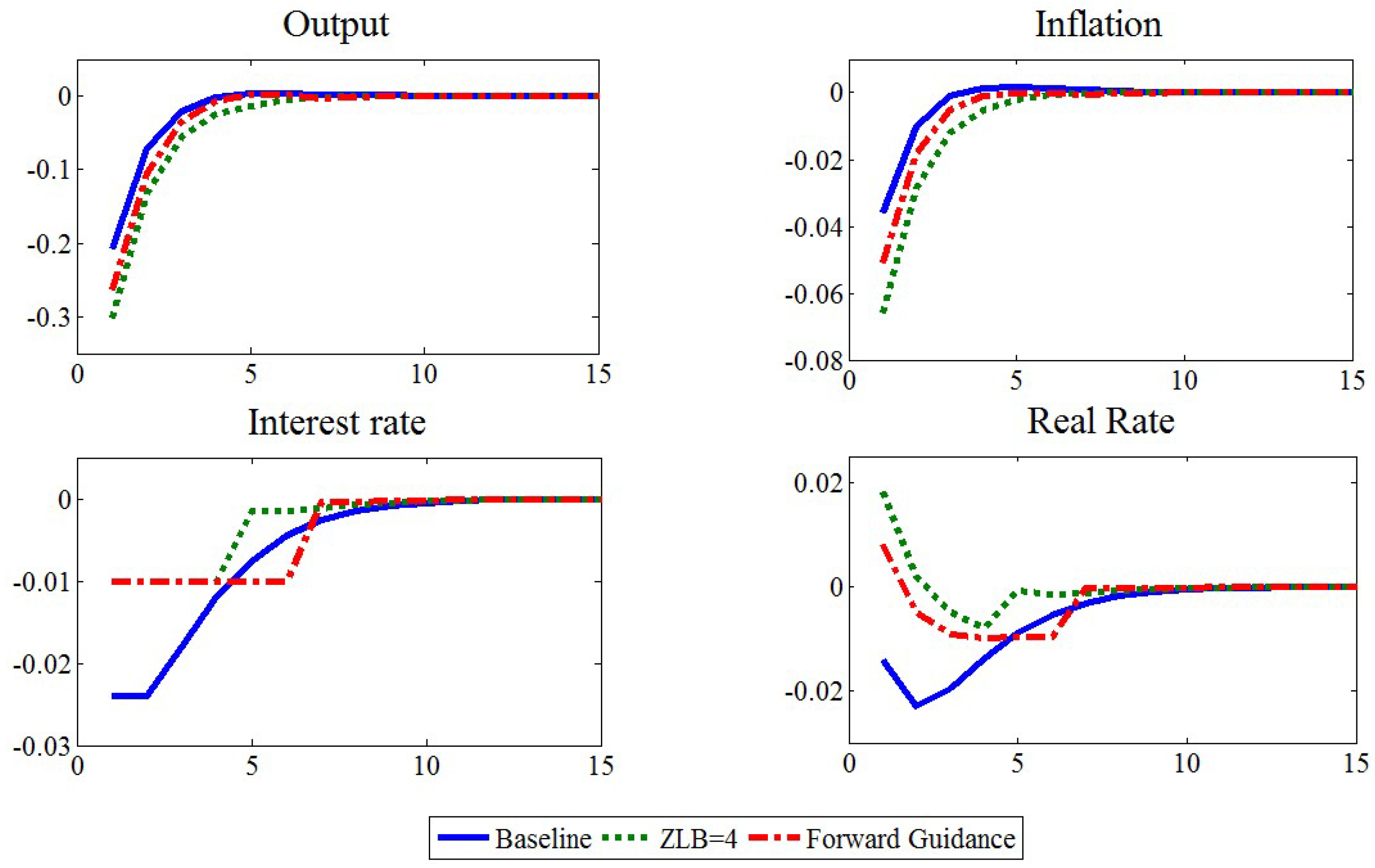
In Figure 1 we depict the dynamic responses of output gap, inflation, short-term nominal interest rate and real rate conditional to a negative preference shock.

The blue line plots the IRF of the variables when we consider a standard New Keynesian model without a zero lower bound. Our IRFs are qualitatively similar to those reported by Galí (2008). In particular, a negative preference shock involves falls in both output and inflation. The central bank tries to countervail the recession by lowering the policy rate, causing a fall also in the real rate, which is the main determinant of consumption. In this environment, monetary policy is effective in stabilizing the economy and smoothing the recession.

If we assume the presence of an occasionally binding constraint, here represented by a zero lower bound, the dynamics of the model variables are affected. The green dotted line depicts these dynamics: in the first four periods following the shock, the zero bound is hit, but the central bank cannot lower the policy rate below zero. As a consequence, we observe a deeper recession (relative to the baseline case) caused by positive real rates due to a strong fall in inflation and the inability of the monetary authority to further lower the nominal rate.

Nonetheless, the central bank can try to alleviate the effect of a binding zero lower bound by using the tool of forward guidance: by making credible statements about how monetary policy will be conducted in the future, the policymaker can influence private sector expectations, exploiting the channel described by Gürkaynak et al. (2005). In our case, we consider a monetary authority announcing that it commits to keeping the policy rate at zero for two further periods beyond what is otherwise required (red dotted line). We still observe a recession, but it is now smaller.

The mechanism behind these dynamics is as follows: by announcing that the policy rate will remain at zero for longer than expected, the central bank can push up private sector expectations about inflation. As a consequence, the real rate increase is restrained, entailing a smaller consumption fall. However, there is no guarantee that announcing policy rates close to zero for many periods will move private sector expectations in the right direction. In fact, agents might interpret the central bank’s choice to keep low policy rates as a signal of a deeper recession and accordingly push down their expectations about the future output gap and inflation.

5. Welfare Analysis

As in the previous section, our welfare study is conducted under the assumption that a negative preference shock hits the economy and pushes down both inflation and the output gap. In the absence of a zero lower bound, the nominal rate would fall below zero for four periods. In the table below, we report the welfare loss associated with several cases.

In the baseline case, we assume there is no zero lower bound, so the nominal rate can fall below zero. ZLB labels the case in which the zero lower bound is binding and the policymaker does not resort to unconventional instruments such as forward guidance. Here, in the four quarters following the shock, it would be optimal to lower the interest rate below zero, but this is not possible due to the presence of a zero lower bound.

The other cases consider a central bank making credible announcements in which it commits to keeping its policy rate at zero for more periods than otherwise requested. For instance, in the case labeled “FG = 2 periods,” we consider a policy rate that remains fixed at zero for 2 additional periods, so in total the short-term rate stays at zero for six periods.

The policy that should be implemented by the monetary authority is the one that minimizes the welfare loss.

From

Table 2. Welfare losses for different durations of the FG.

Model	Welfare Loss	Consumption-Equivalent (%)
Baseline	0.384
ZLB	1.307	0.46
FG = 1 periods	1.121	0.39
FG = 2 periods	0.768	0.26
FG = 3 periods	0.367	0.12
FG = 4 periods	0.218	0.07
FG = 5 periods	1.019	0.35
FG = 6 periods	4.299	1.60

Consumption-equivalent welfare loss is the permanent percentage reduction in steady-state consumption that would make the household indifferent between the ZLB/FG scenario and the baseline (no ZLB) scenario. Calculated following Lucas (2003).

we can observe that the social loss deriving in a world where the zero lower bound is not binding is strongly smaller than that arising when an occasionally binding constraint on the interest rate is considered. This is not surprising as, according to Figure 1, the presence of a zero lower bound has a deflationary effect and provokes a crippling recession (see Eggertsson & Woodford, 2003). When the central bank implements the forward guidance it is able to obtain significant welfare improvements. In fact, apart from the case of a rate equal to zero for ten periods, in all the cases considered herein the welfare loss is significantly smaller than that deriving under the zero lower bound case. Moreover, in some particular cases the central bank is also able to obtain performances better than that observed in the baseline case (when the policy rate is kept to zero for 3 or 4 additional periods). This result, which at first sight might seem weird, derives from the fact that, in general, the Taylor rule could be suboptimal, in particular with respect to optimal policy rules like, e.g., commitment or discretionary policies. When the forward guidance is too long, i.e., 10 periods, it can be harmful to implement it as keeping the rate too far from its fair value could generate an excessively high variability of inflation and output gap. The consumption-equivalent welfare loss for a forward guidance lasting six periods is 1.60% of steady-state consumption, a substantial welfare cost.

5.1. The Destabilizing Effects of Excessively Long Forward Guidance

Why does excessively long forward guidance produce such large welfare losses? The mechanism is an inflationary spiral driven by self-fulfilling expectations.

For a forward guidance lasting three periods, the commitment to keep rates low is sufficiently credible and long enough to raise inflation expectations moderately, reducing the real interest rate and stimulating demand. The economy recovers smoothly, and inflation returns to target without overshooting.

Instead, for a forward guidance lasting six periods, the long commitment generates an explosive dynamic. Agents anticipate that nominal rates will remain at zero for an extended period despite the economy recovering. This leads them to expect substantially higher future inflation. The Phillips curve translates these expectations into current inflation. The central bank, constrained by its commitment, cannot raise rates to counteract the inflation. As inflation rises, real rates fall further, stimulating even more demand. This feedback loop generates a boom-bust cycle: output and inflation overshoot their targets, followed by a sharp contraction when the central bank eventually raises rates.

The resulting volatility is heavily penalized by the quadratic loss function. The variance in inflation in the case with an FG lasting for six periods is more than 15 times larger than in the three periods case. The variance of the output gap is more than 8 times larger. These variances enter the loss function with positive weights, explaining the dramatic increase in welfare loss.

5.2. Sensitivity Analysis

In what follows we implement sensitivity analysis by changing the calibration of our model and investigating how variations in some “deep” parameters affect our results. In particular, we have considered different degrees of price rigidity, lack of interest rate smoothing, absence of central bank response to the output gap, a higher price mark-up, and several levels of risk aversion. In

Table 3. Sensitivity analysis.

	Welfare Loss
Model	θ = 0.5	$\theta$ = 0.75	${\rho }_i$ = 0	${\delta }_y$ = 0	$\epsilon$ = 6	$\sigma$ = 2	σ = 0.5
Baseline	0.446	0.316	0.559	0.530	0.272	0.203	0.746
ZLB	4.814	0.670	1.287	1.388	1.367	0.446	4.841
FG = 1 periods	4.383	0.572	1.106	1.174	1.198	0.373	4.290
FG = 2 periods	2.373	0.427	0.759	0.797	0.770	0.263	2.714
FG = 3 periods	0.236	0.273	0.363	0.378	0.259	0.146	0.819
FG = 4 periods	7.322	0.177	0.219	0.216	0.338	0.084	1.578
FG = 5 periods	61.962	0.250	1.023	1.007	3.006	0.189	14.289
FG = 6 periods	301.863	0.686	4.305	4.279	13.676	0.670	65.226

Each column reports the welfare loss, calculated according to (25), for different calibrations of key parameters in line with what described in Section 5.2.

, we report our results.

We begin our analysis by changing the level of price rigidity. We consider two values for θ, equal to 0.5 and 0.75. In the first case prices are more flexible as they adjust every two quarters (in line with the micro study of Bils & Klenow, 2004), whereas in the second case the degree of rigidity is higher, inducing one price reset per year. When prices are more flexible, the costs of the zero lower bound dramatically go up. This result comes from the fact that now prices are more responsive to an economic slump and, hence, inflation falls more provoking a harder increase in the real rate. This effect could be countervailed by announcing that the policy rate will be kept at zero for a few periods. Also, in this case the forward guidance can involve welfare improvements compared with the baseline case when the nominal rate is kept to zero for three further quarters. On the other hand, when higher price rigidity is considered, welfare losses are restrained. Here, due to stickier prices, inflation falls less and, accordingly, the real rate increases are limited. Again, a forward guidance policy could lead to the best outcomes with respect to the standard case.

In the second experiment we do not consider a central bank that smoothens the interest rate. The effects associated with this change are quite negligible and the welfare losses are similar to that showed in Table 2. Similar results are obtained assuming that the monetary authority moves the policy rate only in response to inflation.

Therefore, we changed the level of price mark-up from 10% to 20%. As in the other scenario considered, the best choice is implementing forward guidance for 3 or 4 periods more than that requested. A policy rate fixed for too long at zero (five or six periods more) entails welfare worsening compared with the ZLB case.

Finally, we consider variations in the parameter encoding the relative risk aversion: changes in σ have important effects because it directly affects the elasticity of the output gap to the real rate (see Equation (17)). Under σ = 2, the output gap is less sensible to real rate change and depends more on expectations over its future value. The contrary happens for σ = 0.5. In the first case, the policymaker’s ability to manage private sector expectations plays a crucial role as, by exploiting the forward guidance channel, he is able to realize smaller welfare losses (also by keeping the policy rate to zero for just one period more). In the second case, the output gap responds more to the real rate; thus, the forward guidance should provide at least zero rates for three additional periods.

Further, we check the robustness to the persistence of the demand shock ${\rho }_z$ and how it affects the optimal FG duration (

Table 4. Robustness to different shocks calibration.

	Welfare Loss
Parameter	Baseline	${\mathit{\rho }}_{\mathit{z}} \mathbf{=} \mathbf{0.3}$	${\mathit{\rho }}_{\mathit{z}} \mathbf{=} \mathbf{0.7}$	${\mathit{\rho }}_{\mathit{a}} \mathbf{=} \mathbf{0}$
Optimal H	4	3	4	3
Min Loss at H*	0.218	0.291	0.201	0.245

The table reports the optimal duration of forward guidance (Optimal H), expressed in additional quarters, for different degrees of shock persistence. Column 3 and 4 check robustness for, respectively, low and high persistence of the demand shock. Column 5 checks robustness for a TFP shock evolving as a white noise shock. “Min loss at H*” indicates the welfare loss achieved in correspondence of the optimal duration of the forward guidance for each degree of inertia considered.

). With ${\rho }_z=0.3$ (less persistent shock), the optimal duration of FG declines to 3 quarters. The economy recovers more quickly, requiring less prolonged stimulus. With ${\rho }_z=0.7$ (more persistent shock), the optimal FG remains at 4 quarters, but the minimal loss is lower (0.201) because the longer-lived shock benefits more from stimulus.

For the technology shock, setting ${\rho }_a=0$ (i.e., technology shocks are i.i.d.) leaves the optimal FG unchanged at 4 quarters. Technology shocks are less important for forward guidance because they affect supply rather than demand; forward guidance primarily operates through the demand channel.

In general, in all the cases considered, we observe that the best choice for the central bank is to act following a forward guidance that fixes the nominal rate to zero for three further quarters as this length is proved to be the one that minimizes the welfare loss and in many cases represents also an improvement with respect to the baseline case. To conclude, excessively long forward guidance generates excessive inflation expectations, increasing macroeconomic volatility and welfare losses.

5.3. Additional Robustness: Stochastic Volatility and Correlated Shocks

To address the concerns raised in Section Limitations of the Baseline Stochastic Specification, we conduct additional robustness analysis.

(1) Stochastic volatility (SV): We model the innovation variance of the preference shock as an AR(1) in logs:

$$ln{\sigma }_{z,t}^2=\left(1-{\rho }_{\sigma }\right)ln{\sigma }_z^2+{\rho }_{\sigma }ln{\sigma }_{z,t-1}^2+{\eta }_t,$$

where ${\eta }_t\sim N\left(0,{\omega }^2\right)$, ${\rho }_{\sigma }=0.9$ and $\omega =0.2$ (calibrated to match uncertainty fluctuations during the 2008 crisis).

(2) Correlated shocks: We introduce correlation between preference and technology shocks, ${\rho }_{z,a}=0.5$ (negative demand shock correlated with negative technology shock).

(3) Bivariate VAR(1): We replace the two independent AR(1) processes with a bivariate VAR(1):

$$\left(\begin{array}{c}{z}_t\\ a_t\end{array}\right)=\left(\begin{array}{c}{\rho }_{zz}\\ {\rho }_{az}\end{array}\begin{array}{c}{\rho }_{za}\\ {\rho }_{aa}\end{array}\right)\left(\begin{array}{c}{z}_{t-1}\\ a_{t-1}\end{array}\right)+\left(\begin{array}{c}{\epsilon }_t^z\\ {\epsilon }_t^a\end{array}\right)$$

with ${\rho }_{zz}=0.5$, ${\rho }_{aa}=0.9$, and cross-persistence ${\rho }_{za}={\rho }_{az}=0.1$.

Table 5. Robustness to alternative stochastic specifications.

Specification	Optimal FG	Minimum Welfare Loss	Change from Baseline
Baseline	4	0.218	-
Stochastic volatility (SV)	3	0.195	−10.5%
Correlated shocks	5	0.267	+22.5%
Bivariate VAR(1)	4	0.221	+1.4%

Optimal duration varies with shock realization; four quarters is the modal outcome. Changes from baseline are expressed in percentage terms as welfare loss differences with respect to the baseline “optimal” duration (four quarters).

summarizes our results.

Under SV, the optimal FG duration falls from 4 to 3 quarters. Heightened uncertainty makes households more precautionary, reducing the effectiveness of FG and making shorter commitments preferable. Under correlated shocks, the optimal FG duration rises to 5 quarters. The supply-side deterioration amplifies the recession, requiring a longer commitment. The optimal FG duration ranges from 3 to 5 quarters depending on the cross-persistence matrix. The baseline optimum of 4 quarters remains representative.

These results indicate that while the precise optimal duration varies with the stochastic specification, the central finding—that optimal FG duration is bounded between 3 and 5 quarters and that extensions beyond 5 quarters generate substantial welfare losses—is robust.

6. Discussion and Policy Implications

6.1. Comparison with Existing Literature

Our results complement and extend existing findings on forward guidance. Eggertsson and Woodford (2003) demonstrated qualitatively that a commitment to keep rates low for an extended period can mitigate the ZLB problem. Our quantitative analysis provides guidance on the magnitude of that extension: 3–4 additional quarters, not longer.

McKay et al. (2016) showed that the power of forward guidance is substantially reduced in incomplete markets models, potentially resolving the forward guidance puzzle. In their framework, long-duration FG (e.g., 5–10 years) produces much smaller effects than in representative-agent models. Our finding that six periods (1.5 years) generate explosive dynamics in a representative-agent model suggests that the forward guidance puzzle may manifest at shorter horizons than previously recognized.

Our robustness analysis relating optimal FG duration to structural parameters (price rigidity, risk aversion, markup) provides a framework for central banks to calibrate their own FG policies based on estimated parameters for their economies. For the euro area, where price rigidity is generally estimated to be higher than in the United States (Galí et al., 2001), our results with θ = 0.75 may be more relevant, suggesting an optimal forward guidance of three quarters.

6.2. Practical Guidance for Central Banks

Our results provide actionable guidance for monetary policymakers. First, forward guidance should be used as a precision tool, not a blunt instrument. The welfare gains from optimal duration (83% reduction in loss relative to no FG) are substantial, but the losses from over-commitment (229% increase in loss for six periods FG) are equally substantial.

Second, the optimal duration depends on the shock’s persistence and the economy’s structural characteristics. In our robustness analysis, the optimal FG varied from 3 to 4 quarters. Central banks should therefore conduct their own welfare-based calculations using their preferred models before committing to a specific FG duration.

Third, forward guidance can be combined with other unconventional policies. Quantitative easing (QE) and negative interest rates (where feasible) might allow a shorter FG commitment or provide insurance against the inflationary risks of prolonged FG. Long-term government bond purchases (quantitative easing) operate through a different channel—reducing term premia and directly lowering long-term yields. When QE is available, the optimal duration of forward guidance can be shorter, because QE provides additional accommodation without requiring commitment to zero short rates for many periods. Conversely, if QE is unavailable (e.g., due to legal constraints or limited bond markets), the required FG duration may need to be longer. Our results assume no QE; thus, they represent an upper bound on the required FG duration when other unconventional tools are absent.

Fourth, communication is critical. Our analysis assumes the forward guidance commitment is perfectly credible. If private agents doubt the central bank’s commitment, the effects will be attenuated. Central banks should therefore structure their forward guidance statements to maximize credibility, for example by tying the commitment to specific economic thresholds (as the Federal Reserve did with its unemployment threshold) rather than calendar dates.

6.3. Empirical Evidence from Central Bank Experience

Our quantitative results find empirical resonance in the actual forward guidance policies implemented by major central banks following the 2008 financial crisis.

If we look at the Federal Reserve Bank in the U.S., in August 2012 the FOMC stated that it expected “exceptionally low levels for the federal funds rate […] at least through mid-2015.” Relative to economic conditions at the time (unemployment above 8%, inflation below target), this represented an extension of approximately 4–5 additional quarters beyond what a standard Taylor rule would prescribe. Williams (2014) estimates that this forward guidance reduced 5-year Treasury yields by 30–40 basis points. Our optimal FG duration of 3–4 quarters is broadly consistent with the Fed’s actual policy. Williams (2014) argued that forward guidance is most effective when tied to economic thresholds (e.g., unemployment or inflation) rather than calendar dates. Our results support this view: optimal FG duration depends on the persistence of the demand shock (${\rho }_z=$ 0.5 in baseline), not on a fixed calendar horizon. Threshold-based guidance allows the duration to adjust automatically to evolving economic conditions. Yellen (2015, speech at the Federal Reserve Bank of San Francisco) emphasized that forward guidance was the primary tool for providing additional accommodation after the federal funds rate reached the ZLB. She noted that the Fed’s 2012–2014 FG was calibrated to the expected duration of the output gap. Our quantitative framework formalizes this calibration exercise.

In August 2013, the Bank of England introduced forward guidance linking interest rates to an unemployment threshold of 7%. The unemployment rate reached 7% in February 2014, making the effective FG duration approximately 3 quarters. Consistent with our results, the BoE’s FG was widely considered effective and did not generate excessive inflationary pressures (Carney, 2013).

The ECB provided forward guidance stating that rates “will remain at present or lower levels for an extended period of time.” This commitment extended for approximately 6–8 quarters. Unlike the Fed and BoE experiences, euro area inflation remained persistently below target (averaging 1% over 2014–2016), suggesting that the FG may have been insufficiently long or insufficiently credible. This is consistent with our finding that optimal FG duration depends critically on the persistence of the demand shock and the credibility of the commitment.

Thus, at the cross-country level what we observed is that no major central bank has implemented FG extensions exceeding 5 quarters without accompanying quantitative easing. Our results suggest that extensions beyond 4 quarters risk generating inflationary volatility, which aligns with observed central bank caution. Central banks that implemented longer FG (ECB) either accompanied it with QE or faced below-target inflation, consistent with our finding that the optimal duration is bounded.

6.4. Macroeconomic Risk and Financial Stability Implications

We have seen that excessively long forward guidance (6+ quarters) can generate high inflation and output volatility.

For an investor, this translates into:

-

Higher long-term bond yield volatility: Term premium risk increases as markets reassess the probability of an inflationary spiral and subsequent sharp rate hikes.

-

Greater uncertainty about real corporate cash flows: Firms face higher uncertainty about future input costs (inflation) and demand (output gap), increasing equity risk premia.

-

Sectoral heterogeneity: Fixed-income sensitive sectors (utilities, real estate) are disproportionately affected by the sharp rate increases that follow prolonged FG.

From a perspective of risk management, our results suggest that whether central banks adopt FG extensions beyond 4 quarters, investors should:

-

Hedge inflation risks using TIPS, inflation swaps, or commodities;

-

Reduce duration exposure in nominal bond portfolios;

-

Increase allocations to assets that perform well under unexpected inflation (e.g., gold, real estate, value stocks);

-

Monitor central bank communication for signs that FG may be extended beyond optimal duration.

What are the implications of our results for financial stability? Excessively long FG may induce search-for-yield behavior, inflating risky asset prices and increasing the risk of a sharp correction when the central bank eventually raises rates. This creates a potential trade-off between short-run output stabilization (which FG achieves) and medium-run financial stability (which prolonged FG may jeopardize).

7. Conclusions

This paper has provided the first systematic welfare-based analysis of the optimal duration of forward guidance at the zero lower bound. Using a New Keynesian DSGE model with a fully specified stochastic environment, we derived three main conclusions.

First, the welfare cost of the ZLB in the absence of forward guidance is substantial: a 240% increase in welfare loss relative to the unconstrained baseline, equivalent to a permanent consumption loss of approximately 0.46%.

Second, forward guidance can dramatically reduce these losses if its duration is appropriately chosen. The optimal commitment extends the zero-rate period by 3–4 additional quarters beyond the Taylor rule’s implied duration. This optimal policy reduces welfare losses by 83% relative to the no-FG ZLB case and even achieves welfare outcomes superior to the unconstrained Taylor rule.

Third, excessively long forward guidance (extensions of 5–6 quarters) generates substantial welfare losses, exceeding both the no-FG ZLB case and the baseline. These losses arise from an inflationary spiral driven by self-fulfilling expectations, which produces large variances in inflation and output.

Our results are robust across alternative calibrations of shock persistence, price rigidity, interest rate smoothing, policy rule parameters, markup, and risk aversion. The optimal duration varies between 3 and 4 quarters across all specifications considered.

Acknowledged limitations: our analysis rests on several assumptions that warrant caution. The representative-agent framework amplifies FG effects relative to incomplete-market economies; the AR(1) shock structure with constant volatility ignores uncertainty clustering during crises; and we assume perfect central bank credibility. Each of these assumptions may affect the optimal duration. We therefore view our quantitative results as a benchmark requiring calibration to specific economic environments rather than a universal prescription. As shown in Section 5.3, under stochastic volatility the optimal duration falls to 3 quarters, while under correlated shocks it rises to 5 quarters. These variations bracket our baseline finding.

These findings have clear implications for central banks implementing forward guidance policies. Forward guidance is a powerful tool, but its power requires precise calibration. Promising low rates for too long risks destabilizing the economy and causing substantial welfare losses. Policymakers should therefore conduct welfare-based calculations to determine the optimal duration for their specific economic environment.

Future research should extend this analysis in several directions. First, incorporating incomplete markets and household heterogeneity would allow us to assess whether the optimal FG duration changes in more realistic environments. Second, adding capital accumulation and investment adjustment costs would provide additional channels for forward guidance to operate. Third, introducing a banking sector and credit friction would allow analysis of the interaction between forward guidance and financial stability. Fourth, estimating the optimal FG duration empirically using Bayesian methods would provide a data-driven benchmark for policy. Fifth, extending the stochastic environment to include time-varying volatility and regime-switching processes would address the limitations discussed in the paper.

Despite these avenues for future work, the core message of this paper is clear: at the zero lower bound, the optimal forward guidance is not simply “more” or “longer,” but rather precisely calibrated to the duration of the underlying shock. For severe demand shocks that would otherwise bind the ZLB for four quarters, three to four additional quarters of zero rates is the welfare-maximizing policy.