A Hybrid HAR-LSTM-GARCH Model for Forecasting Volatility in Energy Markets

Abstract

Accurate volatility forecasting in energy markets is paramount for risk management, derivative pricing, and strategic policy planning. Traditional econometric models like the Heterogeneous Auto-regressive (HAR) model effectively capture the long-memory and multi-component nature of volatility but often fail to account for non-linearities and complex, unseen dependencies. Deep learning models, particularly Long Short-Term Memory (LSTM) networks, excel at capturing these non-linear patterns but can be data-hungry and prone to overfitting, especially in noisy financial datasets. This paper proposes a novel hybrid model, HAR-LSTM-GARCH, which synergistically combines the strengths of the HAR model, an LSTM network, and a GARCH model to forecast the realized volatility of crude oil futures. The HAR component captures the persistent, multi-scale volatility dynamics, the LSTM network learns the non-linear residual patterns, and the GARCH component models the time-varying volatility of the residuals themselves. Using high-frequency data on Brent Crude futures, we compute daily Realized Volatility (RV). Our empirical results demonstrate that the proposed HAR-LSTM-GARCH model significantly outperforms the benchmark HAR, GARCH(1,1), and standalone LSTM models in both statistical accuracy and economic significance, offering a robust framework for volatility forecasting in the complex energy sector.

1. Introduction

The global energy market, with crude oil at its core, constitutes the lifeblood of the modern industrial economy. Its rhythms and shocks reverberate through every facet of global commerce, influencing everything from the geopolitical strategies of nations to the inflation-adjusted budgets of households. At the heart of this complex and often turbulent system lies price volatility—a statistical measure of the dispersion of returns that serves as a fundamental proxy for risk, uncertainty, and market information. The ability to accurately forecast this volatility is not merely an academic exercise; it is a critical imperative for a diverse array of stakeholders. For financial institutions and commodity trading advisors, precise volatility forecasts are the bedrock of derivative pricing, portfolio optimization, and sophisticated risk management frameworks, such as Value-at-Risk (VaR) calculations. For multinational corporations and energy-intensive industries, anticipating price swings is essential for strategic planning, budgeting, and hedging against adverse movements that could erode profit margins. For policymakers and central banks, understanding the trajectory of energy price volatility is crucial for managing national reserves, informing monetary policy, and safeguarding economic stability against external commodity shocks.

The intrinsic characteristics of energy markets, however, render them uniquely challenging to model. Unlike many financial assets, oil prices are subject to a complex and volatile interplay of fundamental forces, including inelastic short-term supply and demand, geopolitical tensions in key producing regions, strategic decisions by cartels like OPEC+, and inventory levels that act as a buffer against disruptions. Furthermore, the financialization of oil over recent decades has meant that prices are also driven by the speculative flows of institutional investors, algorithmic trading, and macroeconomic news, intertwining physical market fundamentals with the often-irrational behavior of financial markets. This confluence of factors gives rise to the well-documented stylized facts of financial volatility, which are particularly pronounced in energy markets: persistent volatility clustering, where periods of high turbulence are followed by more turbulence and calm periods by calm; long memory, where shocks to volatility dissipate at a slow, hyperbolic rate rather than decaying exponentially; and the presence of extreme jumps or breaks, often triggered by unforeseen geopolitical events or macroeconomic announcements.

The quest to model and forecast this volatility has evolved significantly over the past four decades. The pioneering work of Engle (1982) with the Autoregressive Conditional Heteroskedasticity (ARCH) model and its generalization by Bollerslev (1986) into GARCH provided the first formal framework to capture the time-varying nature of volatility and its clustering phenomenon. These models, typically applied to daily returns, represented a monumental leap forward. However, the dawn of the 21st century and the availability of high-frequency data ushered in a new paradigm. The seminal contribution of Andersen and Bollerslev (1998) established Realized Volatility (RV)—constructed from the sum of squared intraday returns—as a more efficient, model-free, and ex-post observable measure of daily volatility. This breakthrough shifted the forecasting problem from predicting a latent variable to forecasting an observed one.

It was within this context that Corsi (2009) introduced the Heterogeneous Autoregressive (HAR) model for Realized Volatility. The HAR model’s elegance and power stem from its remarkable simplicity and its grounding in the Heterogeneous Market Hypothesis. It posits that market participants are heterogeneous, operating over different time horizons (e.g., high-frequency traders, institutional portfolio managers, long-term strategic investors). The HAR model elegantly captures this structure by regressing future daily volatility on lagged daily, weekly, and monthly realized volatilities. Despite its parsimony and linear specification, the HAR model has demonstrated a formidable empirical performance, effectively replicating the long-memory behavior of volatility and becoming a ubiquitous benchmark in the financial econometrics literature, including its successful application to energy markets.

Yet the linear and additive nature of the HAR model is also its primary limitation. The complex, non-linear interactions between the various market agents and the underlying fundamental drivers are forces that a simple linear combination of past volatilities may fail to fully encapsulate. The model may struggle during periods of extreme stress or structural breaks, where the data-generating process itself changes and non-linear dynamics dominate. It is in capturing these intricate, non-linear patterns that a new class of models has shown immense promise.

The recent revolution in artificial intelligence, particularly in deep learning, has opened new frontiers in time-series forecasting. Among these architectures, Long Short-Term Memory (LSTM) networks, a special kind of Recurrent Neural Network (RNN), are uniquely capable. They are explicitly designed to learn long-range dependencies in sequential data, overcoming the vanishing gradient problem that plagued earlier RNNs. Their gated mechanisms allow them to selectively remember and forget information, making them theoretically ideal for financial time series where the relevance of past information can change dynamically. Several studies have begun applying LSTMs directly to volatility forecasting, with some reporting success in capturing complex patterns that elude traditional models.

However, the application of “black-box” deep learning models to the often-noisy and non-stationary domain of financial data is not without peril. Standalone LSTM models can be data-hungry and prone to overfitting on the limited data spans typical of specific market regimes and may fail to consistently outperform robust econometric benchmarks like HAR, which are built upon a solid foundation of financial theory. Their lack of interpretability also remains a significant concern for practitioners who require not just predictions but understanding.

This tension between the theoretical robustness and linear simplicity of econometric models and the flexible, non-linear power of deep learning presents a compelling research opportunity. The most promising path forward lies not in choosing one paradigm over the other nevertheless in their intelligent integration. Hybrid modeling, which seeks to synergize the strengths of different approaches, has emerged as a powerful philosophy. The core idea is decomposition: use a well-specified linear model to capture the primary, persistent component of the series, and then employ a non-linear model to learn the complex residual patterns that the linear model cannot explain.

This paper contributes to this evolving literature by proposing a novel, sequential hybrid framework specifically designed for the challenges of energy market volatility forecasting: the HAR-LSTM-GARCH model. Our approach is a three-stage methodology that builds a more complete and robust forecasting engine. In the first stage, we employ the HAR model as a powerful linear filter, extracting the persistent multi-scale volatility dynamics and yielding a baseline forecast and its associated residuals. In the second stage, we deploy an LSTM network, not on the raw, noisy volatility series, but on the sequence of residuals from the HAR model. This allows the LSTM to focus its considerable pattern-recognition capacity exclusively on the non-linear and complex dependencies that the linear model left behind. The combined HAR-LSTM forecast is then the sum of the linear and non-linear components. Recognizing that the financial innovations from even this sophisticated hybrid may still exhibit the volatility clustering that Engle first identified, we introduce a third stage: fitting a GARCH(1,1) model to the residuals of the HAR-LSTM hybrid. This final layer explicitly models the “volatility of the forecast error,” providing refined, time-varying prediction intervals that enhance the model’s utility for risk management.

Through an empirical application using high-frequency data from the Brent Crude oil market, we demonstrate that this hierarchical integration delivers a significant performance improvement. The proposed HAR-LSTM-GARCH model is shown to outperform the benchmark HAR, a standalone GARCH(1,1), a standalone LSTM model, and a simple two-stage HAR-LSTM hybrid, both in terms of statistical forecast accuracy and the economic relevance of its predictions. This work thus argues for a future of volatility forecasting that is not a contest between econometrics and machine learning but a collaborative synthesis, leveraging the interpretability and structure of the former with the adaptive, non-linear power of the latter to navigate the treacherous but vital waters of the global energy markets.

2. Literature Review

The quest for accurate volatility forecasting has generated a rich and continually evolving literature that bridges financial econometrics, time series analysis, and, more recently, machine learning. This section synthesizes the major developments, from the foundations of econometric volatility models to the latest deep learning and hybrid approaches, with a particular focus on applications in energy markets.

2.1. Evolution of Econometric Volatility Models

The modern study of volatility began with the seminal work of (Engle, 1982), who introduced the Autoregressive Conditional Heteroskedasticity (ARCH) model, formally recognizing that the variance of financial returns is time-varying and predictable. Building on this, Bollerslev (1986) developed the Generalized ARCH (GARCH) model, which became a cornerstone of volatility modeling due to its parsimony and ability to capture persistence. However, these models relied mainly on daily closing prices, overlooking valuable intraday information.

The advent of high-frequency data transformed the field. Andersen and Bollerslev (1998) introduced Realized Volatility (RV) as a non-parametric estimator of daily integrated variance, allowing volatility to be observed directly. This innovation paved the way for new forecasting approaches, notably the Heterogeneous Autoregressive (HAR) model proposed by Corsi (2009). Based on the Heterogeneous Market Hypothesis, the HAR model captures volatility’s long-memory behavior using lagged daily, weekly, and monthly RV components and remains a leading benchmark.

Applied to energy markets, these models highlight the unique characteristics of commodities such as oil and gas. Studies by Sévi (2014) and Prokopczuk et al. (2016) revealed that energy volatility exhibits stronger persistence and jump components than equity volatility. Building on this, Degiannakis and Filis (2017) showed that HAR-type models that explicitly separate continuous and jump components of RV achieve superior forecasts, underscoring the need to model the discontinuous nature of oil price movements.

2.2. Rise of Machine and Deep Learning in Financial Forecasting

In parallel, the rapid advancement of machine learning (ML) has revolutionized financial forecasting. Initial efforts using Support Vector Machines (SVM) and Multilayer Perceptrons (MLP) soon gave way to deep learning architectures better suited for sequential and nonlinear financial data.

Among these, Long Short-Term Memory (LSTM) networks-introduced by Hochreiter and Schmidhuber (1997)-stand out for their ability to learn long-term dependencies through gated mechanisms that mitigate the vanishing gradient problem. A comprehensive survey by (Sezer et al., 2020) documented the consistent superiority of LSTM and related deep models over traditional econometric approaches in forecasting of volatility.

Recent applications in energy markets reinforce these findings. For example, Song et al. (2022) employed Equity Market Volatility (EMV) trackers derived from news data to predict crude oil market volatility, finding petroleum-specific EMV indices to be the most effective predictors. Similarly, Mohsin and Jamaani (2023) proposed GroupNet, a deep convolutional neural network that combines convolutional and regression layers to forecast crude oil prices based on precious metal data, achieves higher accuracy than both machine learning and statistical benchmarks. Other works have advanced this line of research. Jin and Xu (2024) applied nonlinear auto-regressive neural networks to forecast WTI and Brent crude oil, natural gas, and heating oil prices, achieving remarkably low relative RMSEs (below 2% for crude oils). Likewise, Sen and Choudhury (2024) optimized the hyperparameters of LSTM and GRU models using Particle Swarm Optimization, finding that GRU outperformed LSTM. More recently, Yu et al. (2025) developed a dynamic factor model using Incremental Principal Component Analysis (IPCA) to extract key drivers of crude oil option prices. Combining eight machine learning algorithms through a weighted hybrid model and explaining results via SHAP analysis, the study improved both accuracy and interpretability.

2.3. Emergence and Rationale of Hybrid Models

Hybrid modeling has gained prominence as an effective remedy to the shortcomings of standalone deep learning models, whose opacity, noise sensitivity, and tendency to overfit often limit their usefulness in financial forecasting. Inspired by the decomposition-and-ensemble paradigm of (Zhang, 2003), recent research increasingly blends econometric and machine learning techniques to separate time series into linear and nonlinear components, allowing each to be modeled with the most appropriate tool. Within this perspective, several influential studies have achieved notable improvements in forecasting performance across financial and energy markets. Initial work, such as (Roh, 2007), combined GARCH-family estimators with artificial neural networks, demonstrating that hybrids like NN-GARCH could outperform standalone neural networks on metrics such as MAE. The paradigm has since advanced with deep learning, particularly through the integration of LSTM networks with GARCH models to jointly capture long-memory patterns and conditional heteroskedasticity (Kristjanpoller et al., 2014; Bhattacharya & Ahmed, 2018; Kim & Won, 2018; Y. Hu et al., 2020). Further innovations combine stochastic volatility (SV) with recurrent architectures (Nguyen et al., 2023). While Boubaker and Bannour (2023) propose an ARFIMA-WLLWNN hybrid that fuses long-memory dynamics, wavelet decomposition, and neural networks to predict stock market returns and volatility, outperforming multiple benchmarks on Dow Jones data. Similarly, Mtiraoui et al. (2023) develop an ARFIMA–EWLLWNN framework optimized via backpropagation and particle swarm methods for Bitcoin forecasting, while Ben Amor et al. (2018) apply a k-factor GARMA–EWLLWNN model to Polish electricity prices with substantial accuracy gains. More recently, Ladhari and Boubaker (2024) introduce hybrid LSTM-Attention and ANN-LSTM architectures enhanced through gradient-specific optimization, showing superior adaptability to rapid price fluctuations. The hybrid approach has been particularly impactful in volatility forecasting: early evidence from Donaldson and Kamstra (1997) demonstrated that GARCH–ANN systems surpass their individual components, and subsequent contributions such as (Aldabagh et al., 2023) confirm the strength of CNN–LSTM hybrids for crude oil modeling, even under extreme market conditions like COVID-19 or geopolitical shocks. Nsengiyumva et al. (2025) introduce a hybrid GARCH-LSTM model for Value at Risk (VaR) forecasting in Rwanda’s foreign exchange market. Evaluated on USD, EUR, and GBP data, the hybrid outperforms standalone models, boosting VaR accuracy by up to 10% during high volatility. Furtheremore Vo (2025) compares five deep learning models to the HAR benchmark for volatility forecasting, using major U.S. indices and macroeconomic data. Key findings show DL models significantly outperform HAR only when macroeconomic variables are included, with TiDE and DeepAR excelling at different horizons. Additional advances include (Pan et al., 2025), who improve WTI volatility prediction using a wavelet-filtered Hybrid HAR-RV model, and G. Hu et al. (2025), who design ML-HAR-RV hybrids for China’s crude oil futures that leverage signed jumps to enhance performance during stress episodes. Parallel efforts merge HAR models with machine learning, exemplified by Zhuo and Morimoto (2024), who combine HAR with Support Vector Regression to better capture stock market volatility. Overall, this expanding body of work underscores the growing relevance and effectiveness of hybrid econometric-machine learning frameworks in improving interpretability, robustness, and forecasting accuracy. However, a critical gap remains in the existing literature. While some studies have combined HAR with LSTMs, they often do so in a parallel or feature-engineering capacity, rather than the sequential residual-modeling approach we propose. Furthermore, few models explicitly address the conditional heteroskedasticity that may persist in the residuals of the primary hybrid forecast. This is a significant oversight, as ignoring this “volatility-of-volatility” can lead to misspecified confidence intervals and sub-optimal risk management decisions. The GARCH-in-Mean model has been used to incorporate volatility into the mean equation, but using a GARCH process to model the residuals of a deep learning model is a novel refinement.

Our proposed HAR-LSTM-GARCH model directly addresses this gap. It builds upon the established strength of the HAR model as a feature generator, leverages the state-of-the-art pattern recognition of LSTM for non-linear residual modeling, and introduces a final GARCH layer to ensure the model’s innovation process is well-behaved, thereby providing a more complete and robust framework for energy volatility forecasting.

3. Data and Methodology

This section provides a comprehensive exposition of the data collection process, the construction of volatility measures, and the complete methodological framework for the proposed hybrid model. The approach is deliberately structured to leverage daily data, making the methodology accessible and computationally feasible while retaining the core insights from high-frequency data through carefully constructed realized volatility estimators. The entire forecasting workflow, from raw data to the final HAR-LSTM-GARCH forecast, is delineated in a sequential, step-by-step manner.

3.1. Data Source and Daily Realized Volatility Construction

The empirical analysis is conducted on the Brent Crude Oil spot price, a leading global benchmark for oil prices. Daily closing prices, denoted as $P_t$, are sourced for the period from 4 January 2010, to 30 December 2022. This extensive timeframe encompasses several distinct market regimes, including periods of relative stability, the shale revolution, the unprecedented negative price shock in April 2020, and the subsequent recovery marked by high volatility due to geopolitical conflicts. Utilizing daily data ensures a long and consistent time series, which is crucial for both the robust estimation of econometric models and the effective training of data-intensive deep learning networks.

The raw price series is first transformed into a daily log-return series, $r_t$, which serves as the fundamental building block for all subsequent volatility measures. The transformation is given by:

$$r_t=ln\left({\displaystyle \frac{P_t}{P_{t-1}}}\right)\times 100$$

(1)

where the multiplication by 100 converts the returns into percentage terms, which standardizes the scale and aids in numerical stability during model estimation. The resulting series ${\left\{r_t\right\}}_{t=1}^T$ is then subjected to standard cleaning procedures to remove any potential data errors and to ensure the integrity of the analysis.

The concept of Realized Volatility (RV), as introduced by (Andersen & Bollerslev, 1998), is based on the theory of quadratic variation. In an ideal setting with frictionless markets and no microstructure noise, the sum of squared intraday returns provides a model-free, ex-post consistent estimator of the day’s integrated variance. However, in the absence of high-frequency data, a common and robust practice in the literature is to proxy the unobserved daily integrated variance using the squared daily return.

While this is a noisy estimator for a single day, its performance improves significantly when aggregated over intervals. Therefore, we define the daily dealized volatility for day t simply as the rolling standard deviation with a window of 22 days of the squared daily return:

$$R{V}_t^{daily}=\sqrt{{\displaystyle \frac{252}{22}}\sum _{i=1}^{22}{r}_t^2}$$

(2)

This measure, $R{V}_t^{daily}$, captures the instantaneous variance on day t. Although it is a noisy measure for any single day, its expectation is equal to the true conditional variance, and it becomes the foundational element for constructing the persistent volatility components required by the HAR model.

Based on the

Table 1. Descriptive statistics of returns and realized volatility series.

	Daily Reurns	Realizd Volatility
Nbr.obs	4366	4345
Mean	0.0000	0.2745
Median	0.0000	0.2292
Std.dev	0.0205	0.1759
Skewness	−0.1819	3.5191
Kurtosis	10.1876	17.1252
Jarque Bera	18,927.1113	62,126.0717
Arch(10)	1454.3248	4303.1616

, the data exhibits several key characteristics typical of financial time series. The daily returns show a mean near zero with moderate standard deviation, indicating no significant drift but considerable day-to-day variability. The realized volatility series displays a much higher mean and standard deviation, reflecting the substantial fluctuation in market volatility levels over the observation period.

Both series demonstrate significant non-normality, as evidenced by high skewness and kurtosis values. The realized volatility shows extremely positive skewness (3.52) and high kurtosis (17.13), indicating a right-skewed distribution with heavy tails and frequent extreme values. The Jarque-Bera test statistics are exceptionally large for both series, strongly rejecting the null hypothesis of normality.

Most notably, the ARCH test statistics are highly significant (1454 for returns and 4303 for volatility), providing strong evidence of volatility clustering. This suggests that large price movements tend to be followed by large movements, and small changes tend to be followed by small changes, confirming the presence of conditional heteroskedasticity in the data. These findings justify the application of GARCH-type models and the hybrid HAR-LSTM-GARCH framework proposed in the study.

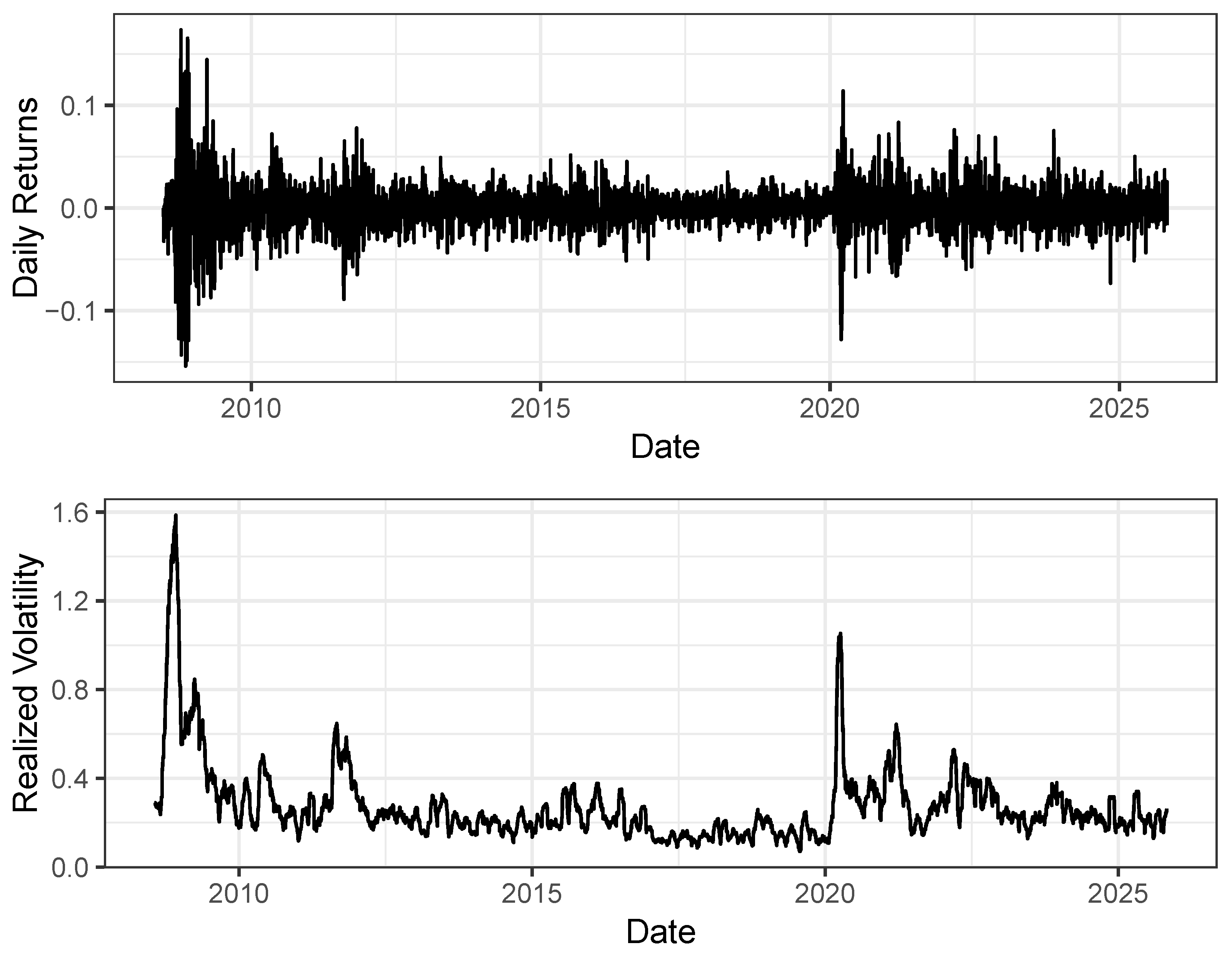
The time series plots (Figure 1) reveal key stylized facts of financial returns and volatility. The daily returns series exhibits the characteristic volatility clustering phenomenon, where periods of high volatility (e.g., 2008–2009, 2020) are followed by relative calm. The realized volatility plot shows dramatic spikes during market stress periods, particularly the extreme peak in 2008 corresponding to the financial crisis market crash.

Both series demonstrate persistent behavior, with volatility appearing to be highly auto-correlated over time. The visual evidence strongly supports the presence of time-varying volatility and heteroskedasticity in the data, justifying the need for sophisticated modeling approaches like the proposed HAR-LSTM-GARCH framework to capture these complex dynamics. The extreme movements in both series align with the high kurtosis and significant ARCH effects identified in the statistical analysis.

3.2. Constructing Heterogeneous Volatility Components with a Rolling Window

The seminal contribution of the HAR model by (Corsi, 2009) is its ability to parsimoniously capture the long-memory behavior of volatility by incorporating the actions of heterogeneous market participants operating over different time horizons. To empirically implement this structure, we construct weekly and monthly volatility components by aggregating the daily $R{V}_t^{daily}$ over relevant horizons. A key methodological choice is the width of the rolling window used for this aggregation. Following standard financial practice, we define a trading month as comprising 22 business days and a trading week as 5 business days.

The volatility components are constructed using a backward-looking rolling window of width 22 days, ensuring that each component is a function of exactly one trading month of the most recent data. The components are defined as follows:

• Daily Volatility Component ($R{V}_t$): This is simply the most recent observation of the daily realized volatility.

  $$R{V}_t^d=R{V}_t^{daily}$$

  (3)
• Weekly Volatility Component ($R{V}_t^w$): This component reflects the volatility over the past trading week (5 days). It is constructed as the simple average of the last 5 days of daily realized volatility.

  $$R{V}_t^w={\displaystyle \frac{1}{5}}\sum _{i=0}^{4}R{V}_{t-i}^{daily}$$

  (4)
• Monthly Volatility Component ($R{V}_t^m$): This component captures the longer-term volatility trend over the past trading month (22 days). It is constructed as the simple average of the last 22 days of daily realized volatility.

  $$R{V}_t^m={\displaystyle \frac{1}{22}}\sum _{i=0}^{21}R{V}_{t-i}^{daily}$$

  (5)

This rolling window approach ensures that all components are available in real-time for forecasting and that the model adapts to changing market conditions. The final dataset for model estimation is a triple $\{R{V}_t^d,R{V}_t^w,R{V}_t^m\}$ for each day t, where t runs from the 23rd observation (to allow for the initial 22-day window) to the end of the sample. The target variable for forecasting is the one-day-ahead realized volatility, $R{V}_{t+1}$.

3.3. The Benchmark Models

To establish a rigorous baseline for evaluating the performance of the proposed hybrid model, we implement three well-established benchmark models from the financial econometrics and machine learning literature.

3.3.1. The Heterogeneous Autoregressive (HAR) Model

The HAR model is a workhorse in the realized volatility literature due to its simplicity and empirical robustness. It is specified as a linear additive model that regresses future volatility on the three heterogeneous volatility components. The model is based on the idea that the volatility process is driven by the interactions of traders with different time horizons, and these interactions induce a persistent hyperbolic decay in the autocorrelation function of volatility.

The mathematical formulation of the HAR model for one-day-ahead forecasting is:

$$R{V}_{t+1}={\beta }_0+{\beta }_{d}R{V}_t^d+{\beta }_{w}R{V}_t^w+{\beta }_{m}R{V}_t^m+{ϵ}_{t+1}$$

(6)

where $R{V}_{t+1}$ is the realized volatility to be forecasted for day $t+1$, ${\beta }_0$ is the model intercept. ${\beta }_d$, ${\beta }_w$, and ${\beta }_m$ are the parameters capturing the sensitivity of future volatility to the daily, weekly, and monthly components, respectively, and ${ϵ}_{t+1}$ is the error term assumed to be independently and identically distributed with mean zero and constant variance.

The one-day-ahead point forecast from the HAR model is given by:

$${\widehat{RV}}_{t+1}^{HAR}={\widehat{\beta }}_0+{\widehat{\beta }}_{d}R{V}_t+{\widehat{\beta }}_{w}R{V}_t^w+{\widehat{\beta }}_{m}R{V}_t^m$$

(7)

where the parameters $\widehat{\beta }$ are estimated via Ordinary Least Squares (OLS) regression. The HAR model serves as our primary econometric benchmark, representing the state-of-the-art in parsimonious linear volatility forecasting.

3.3.2. The GARCH Model

The Generalized Auto-regressive Conditional Heteroskedasticity (GARCH) model of (Bollerslev, 1986) is the cornerstone of conditional variance modeling. Unlike the HAR model, which forecasts a directly observable variable (RV), the GARCH model forecasts the latent conditional variance of returns. It captures the well-documented phenomenon of volatility clustering-where periods of high volatility tend to be followed by more high volatility, and vise versa.

The GARCH(1,1) model for the return series $r_t$ is specified as follows:

Mean Equation:

$$r_t=\mu +{\eta }_t,{\eta }_t={\sigma }_t{\nu }_t,{\nu }_t\sim N(0,1)$$

(8)

Variance Equation:

$${\sigma }_t^2=\omega +\alpha {\eta }_{t-1}^2+\beta {\sigma }_{t-1}^2$$

(9)

where $\mu$ is the constant mean return, ${\eta }_t$ is the error term, ${\sigma }_t^2$ is the conditional variance at time t, $\omega >0$ is the constant term, $\alpha \ge 0$ captures the reaction of volatility to past shocks (the ARCH effect) and $\beta \ge 0$ captures the persistence of volatility (the GARCH effect). The persistence of the volatility process is measured by $\alpha +\beta$, with values close to 1 indicating highly persistent volatility.

The one-day-ahead forecast of the conditional variance is:

$${\widehat{\sigma }}_{t+1}^2=\widehat{\omega }+\widehat{\alpha }{\eta }_t^2+\widehat{\beta }{\sigma }_t^2$$

(10)

This forecast, ${\widehat{\sigma }}_{t+1}^2$, serves as the GARCH benchmark forecast. It is important to note that while the target variable differs from the HAR model (${\sigma }_t^2$ vs. $R{V}_t$), the GARCH model provides a crucial benchmark for a different class of volatility models.

The specification for the benchmark GARCH model was determined through a standard model selection procedure to ensure a robust and representative econometric baseline. We evaluated a set of candidate $GARCH(p,q)$ models (with $p,q\le 2$) under various conditional error distributions, including the Normal, Skewed Normal, Student’s, and Skewed Student’s. Each candidate was estimated on the full training sample of daily returns, and model selection was guided by the RMSE criteria. The process identified the standard $GARCH(1,1)$ specification with a Skewed Student’s conditional distribution as the most appropriate benchmark. The fitted parameters of the optimal benchmark $GARCH(1,1)$ model, estimated via maximum likelihood, are presented in

Table 2. Parameter Estimates of GARCH model.

	Estimate	Std. Error	t Value	Pr(>|t|)
omega	0.0036	0.0006	5.8818	0.0000
alpha1	0.1574	0.0393	4.0051	0.0000
beta1	0.6653	0.0143	46.4668	0.0000
skew	0.2121	0.0062	34.0922	0.0000
shape	2.5027	0.0252	99.1997	0.0000

. All coefficients are highly statistically significant ($p<0.001$).

To ensure a comprehensive comparison and to explicitly model the asymmetric impact of news on volatility—a well-documented feature in energy markets—we also implement a GJR-GARCH(1,1) model as an additional benchmark. Proposed by (Glosten et al., 1993), this model extends the standard GARCH framework by incorporating a leverage term that allows negative and positive return shocks to have differential effects on future volatility. The variance equation is specified as:

$${\sigma }_t^2=\omega +\alpha {\epsilon }_{t-1}^2+\gamma {\epsilon }_{t-1}^2{I}_{t-1}+\beta {\sigma }_{t-1}^2$$

(11)

where $I_{t-1}$ is an indicator function that equals 1 if ${\epsilon }_{t-1}<0$ (bad news) and 0 otherwise. The parameter $\gamma >0$ captures the additional volatility impact of negative shocks (the leverage effect). This model serves as a more nuanced and realistic nonlinear benchmark against which to evaluate the proposed HAR-LSTM-GARCH framework, testing whether the LSTM component provides forecasting benefits beyond what is achievable with established parametric models of volatility asymmetry.

3.3.3. The Stochastic Volatility Model

The Stochastic Volatility (SV) model provides a framework for analyzing a zero-mean return series $r_t=(r_1,r_2,\dots ,r_n)$ by introducing a unique, time-specific variance $e^{h_t}$ for each observation $r_t$. To impose structure, the log-variance $h_t$ is assumed to follow an autoregressive process of order one. This stochastic evolution of volatility is the defining characteristic that separates the SV model from GARCH-type alternatives, which model volatility through a deterministic equation. The log volatility $h_t$ is modeled as follows:

$$\begin{array}{cc}\hfill r_t& ={\epsilon }_{t}exp\left({\displaystyle \frac{h_t}{2}}\right),t=1,\dots ,n,\hfill \end{array}$$

(12)

$$\begin{array}{cc}\hfill h_{t+1}& =\mu +\varphi (h_t-\mu )+{\eta }_t,t=1,\dots ,n-1,\left|\varphi \right|<1,\hfill \end{array}$$

(13)

$$\begin{array}{cc}\hfill h_1& \sim \mathcal{N}\left(\mu ,{\displaystyle \frac{{\sigma }_{\eta }^2}{1-{\varphi }^2}}\right),\hfill \end{array}$$

(14)

$$\begin{array}{cc}\hfill {\epsilon }_t& \sim \mathcal{N}(0,1),\hfill \end{array}$$

(15)

$$\begin{array}{cc}\hfill {\eta }_t|{\epsilon }_t& \sim \mathcal{N}\left(\rho {\sigma }_{\eta }{\epsilon }_t,(1-{\rho }^2){\sigma }_{\eta }^2\right)\hfill \end{array}$$

(16)

where $\varphi$ is the persistence parameter of the log-volatility process and $\mu$ is the unconditional mean of log-volatility.

To ensure stationarity, the persistence parameter is constrained to $\left|\varphi \right|<1$. Consequently, the initial state $h_1$ is drawn from the unconditional (stationary) distribution of the process.

The innovation terms ${\epsilon }_t$ and ${\eta }_t$ follow a bivariate normal distribution,

$$\left(\begin{array}{c}{\epsilon }_t\\ {\eta }_t\end{array}\right)\sim \mathcal{N}\left(\left(\begin{array}{c}0\\ 0\end{array}\right),\left(\begin{array}{cc}1& \rho {\sigma }_{\eta }\\ \rho {\sigma }_{\eta }& {\sigma }_{\eta }^2\end{array}\right)\right),$$

where $\rho$ is the correlation coefficient. This structure directly incorporates the leverage effect, a key empirical feature in financial markets. When $\rho <0$, a negative return shock (${\epsilon }_t<0$) is likely to coincide with a positive innovation in log-volatility (${\eta }_t>0$), leading to an increase in future volatility $h_{t+1}$. This captures the observed asymmetry where bad news (negative returns) tends to increase future volatility more than good news.

3.3.4. The Standalone LSTM Model

Long Short-Term Memory (LSTM) networks, introduced by (Hochreiter & Schmidhuber, 1997), are a specialized form of Recurrent Neural Networks (RNNs) designed to model long-range dependencies in sequential data. Their architecture includes a memory cell and three gating mechanisms (input, forget, and output gates) that regulate the flow of information, allowing them to learn which information in a sequence is important to retain or discard over long periods. This makes them theoretically ideal for financial volatility, which exhibits long memory.

The standalone LSTM model is implemented to forecast $R{V}_{t+1}$ directly using the same input features as the HAR model. However, unlike the linear HAR model, the LSTM can learn complex, non-linear functional mappings. The input to the model at time t is a sequence of the past L observations of the feature vector ${\mathbf{x}}_t=[R{V}_t^d,R{V}_t^w,R{V}_t^m]$. This creates a three-dimensional input tensor of shape (samples, L, 3).

The core operations within a single LSTM cell for a time step i are mathematically defined as follows:

Forget Gate: Determines what information to discard from the cell state.

$${\mathbf{f}}_i=\sigma ({\mathbf{W}}_f·[{\mathbf{h}}_{i-1},{\mathbf{x}}_i]+{\mathbf{b}}_f)$$

(17)

Input Gate: Determines what new information to store in the cell state.

$$\begin{array}{cc}\hfill {\mathbf{i}}_i& =\sigma ({\mathbf{W}}_i·[{\mathbf{h}}_{i-1},{\mathbf{x}}_i]+{\mathbf{b}}_i)\hfill \end{array}$$

(18)

$$\begin{array}{cc}\hfill {\tilde{\mathbf{C}}}_i& =tanh({\mathbf{W}}_C·[{\mathbf{h}}_{i-1},{\mathbf{x}}_i]+{\mathbf{b}}_C)\hfill \end{array}$$

(19)

Cell State Update: Combines the previous cell state and the new candidate values.

$${\mathbf{C}}_i={\mathbf{f}}_i\odot {\mathbf{C}}_{i-1}+{\mathbf{i}}_i\odot {\tilde{\mathbf{C}}}_i$$

(20)

Output Gate: Determines what part of the cell state to output.

$$\begin{array}{cc}\hfill {\mathbf{o}}_i& =\sigma ({\mathbf{W}}_o·[{\mathbf{h}}_{i-1},{\mathbf{x}}_i]+{\mathbf{b}}_o)\hfill \end{array}$$

(21)

$$\begin{array}{cc}\hfill {\mathbf{h}}_i& ={\mathbf{o}}_i\odot tanh\left({\mathbf{C}}_i\right)\hfill \end{array}$$

(22)

Here, $\sigma$ is the sigmoid activation function, ⊙ denotes the Hadamard (element-wise) product, $\mathbf{W}$ and $\mathbf{b}$ are weight matrices and bias vectors, ${\mathbf{x}}_i$ is the input, ${\mathbf{h}}_i$ is the hidden state, and ${\mathbf{C}}_i$ is the cell state.

The final LSTM output, ${\mathbf{h}}_L$, is passed through a final dense layer with a linear activation to produce the volatility forecast:

$${\widehat{RV}}_{t+1}^{LSTM}={\mathbf{W}}_{out}{\mathbf{h}}_L+b_{out}$$

(23)

The model is trained to minimize the Mean Squared Error (MSE) between its predictions and the actual realized volatility.

3.3.5. The Neural Network GARCH Model

To provide a robust comparison against modern hybrid approaches, we implement an Neural Network GARCH (NN-GARCH) model as an additional benchmark, representing the class of hybrid models that integrate neural networks with GARCH volatility modeling (Donaldson & Kamstra, 1997; Kristjanpoller & Minutolo, 2016). The model is implemented in two sequential stages. First, an Artificial Neural Network (ANN) with a single hidden layer is fitted to forecast returns using lagged returns as inputs; its hyperparameters (number of hidden units, weight decay) are optimized via 5-fold cross-validation to minimize out-of-sample prediction error. The residuals from this ANN forecast are then extracted. In the second stage, a GARCH(1,1) model with a Skewed Normal distribution is fitted to these residuals to capture their conditional heteroskedasticity. The final forecast is obtained by combining the ANN point prediction with the GARCH-based volatility forecast.

3.4. The Proposed HAR-LSTM-GARCH Hybrid Model

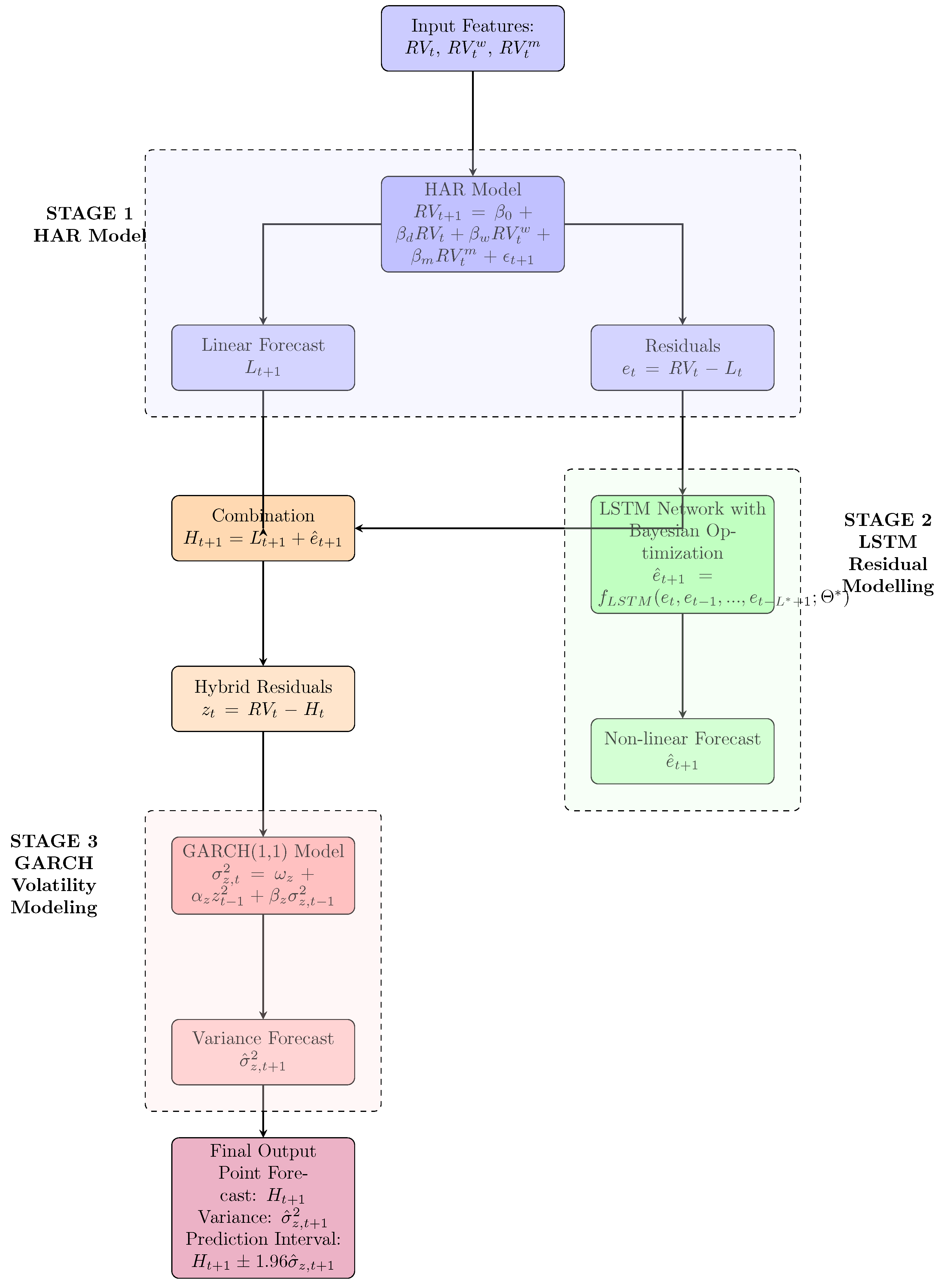
The proposed hybrid model is a three-stage sequential framework designed to synthesize the strengths of its individual components. The core philosophy is one of decomposition: the HAR model captures the persistent linear structure, the LSTM models the non-linear residuals, and the GARCH model accounts for the remaining heteroskedasticity in the forecast errors. The architectural flow is illustrated in Figure 2 and described in detail in the following subsections.

3.4.1. Stage 1: HAR Model Fitting and Residual Extraction

In the first stage, the HAR model is employed as a sophisticated linear filter. It is fitted to the entire training dataset to obtain parameter estimates ${\widehat{\beta }}_0,{\widehat{\beta }}_d,{\widehat{\beta }}_w,{\widehat{\beta }}_m$. The model is then used to generate in-sample forecasts for each day t in the training set:

$$L_t={\widehat{\beta }}_0+{\widehat{\beta }}_{d}R{V}_{t-1}+{\widehat{\beta }}_{w}R{V}_{t-1}^w+{\widehat{\beta }}_{m}R{V}_{t-1}^m$$

(24)

Note that the features are lagged by one period to maintain a strict out-of-sample forecasting structure, even for in-sample fits. The residual series $\left\{e_t\right\}$, which represents the component of volatility that the linear HAR model cannot explain, is then computed:

$$e_t=R{V}_t-L_t$$

(25)

This residual series is the critical input for the second stage of the hybrid model. It contains the non-linear dependencies, structural breaks, and complex patterns that are beyond the scope of a linear model.

The inclusion of the LSTM component in the second stage is predicated on the presence of significant nonlinear dependencies in the residuals of the linear HAR model. To formally test this hypothesis, we employ the McLeod-Li test (McLeod & Li, 1983).

The McLeod-Li test is a portmanteau test applied to the squared residuals of a time series model. For a series of residuals $e_t$ from the HAR model, the test statistic checks for autocorrelation in the squared residuals up to a specified lag m:

$$Q^{*}\left(m\right)=n(n+2)\sum _{k=1}^m{\displaystyle \frac{{\widehat{\rho }}^2\left(k\right)}{n-k}}$$

(26)

where n is the sample size, and $\widehat{\rho }\left(k\right)$ is the sample autocorrelation of the squared residuals at lag k. Under the null hypothesis that the residuals are independent and identically distributed (i.i.d.), the test statistic asymptotically follows a ${\chi }^2\left(m\right)$ distribution.

Applying the McLeod-Li test to the standardized residuals of the HAR model yields a test statistic of $Q^{*}\left(20\right)=4869.184$ with a p-value below 0.001. This provides strong statistical evidence to reject the null hypothesis of i.i.d. residuals, indicating the presence of significant nonlinear dependence—specifically in the form of persistent autocorrelation in squared residuals.

3.4.2. Stage 2: LSTM for Non-Linear Residual Modeling with Bayesian Optimization

The second stage is dedicated to learning the non-linear patterns embedded within the residual series $\left\{e_t\right\}$. An LSTM network is tasked with forecasting the future residual $e_{t+1}$. To achieve optimal performance, the architecture and hyperparameters of the LSTM are not chosen arbitrarily but are systematically tuned using Bayesian optimization.

Bayesian Optimization Framework: To systematically identify the optimal hyperparameters for the LSTM network, we employed Bayesian Optimization. This approach constructs a probabilistic surrogate model of the objective function—using a Gaussian Process (GP) with a Matern $5/2$ kernel—to efficiently navigate the hyperparameter space. The optimization was configured to minimize the Mean Squared Error (MSE) of the LSTM’s one-step-ahead forecasts on a held-out validation set (constituting 15% of the training data).

The hyperparameter search space is defined as:

• Number of Units: $Units\in [10,100]$ (integers).
• Learning Rate: $lr\in [1\times {10}^{-4},1\times {10}^{-2}]$ (log scale).
• Batch Size: $b\in [8,64]$ (integers).
• Epochs: $E\in [20,500]$ (integers).

The optimization algorithm runs for a fixed number of trials (e.g., 20), and for each trial, an LSTM model with a specific hyperparameter configuration is trained on the training residuals and evaluated on a validation set. The configuration that minimizes the validation Mean Squared Error (MSE) is selected.

LSTM Training and Forecasting: With the optimal hyperparameters ${\mathsf{\Theta }}^{*}$ found, the final LSTM model is trained on the entire set of training residuals. The input is a sequence of the past $L^{*}$ residuals, $[e_t,e_{t-1},...,e_{t-L^{*}+1}]$, and the target is the next residual, $e_{t+1}$. The LSTM learns a non-linear function $f_{LSTM}$ such that:

$${\widehat{e}}_{t+1}=f_{LSTM}(e_t,e_{t-1},...,e_{t-L^{*}+1};{\mathsf{\Theta }}^{*})$$

(27)

The hybrid HAR-LSTM point forecast is then obtained by combining the linear forecast from Stage 1 with the non-linear residual forecast from Stage 2:

$$H_{t+1}=L_{t+1}+{\widehat{e}}_{t+1}$$

(28)

A new series of residuals is computed from this hybrid forecast:

$$z_t=R{V}_t-H_t$$

(29)

This series $\left\{z_t\right\}$ represents the final, unexplained component of the volatility after both linear and non-linear modeling.

3.4.3. Stage 3: GARCH Modeling of the Hybrid Residuals

The third and final stage acknowledges that the residuals from the HAR-LSTM model, $\left\{z_t\right\}$, may still exhibit conditional heteroskedasticity. This is a common feature in financial time series, where the errors of a mean model are not i.i.d. but have time-varying variance. Ignoring this can lead to inefficient forecasts and incorrect prediction intervals.

To capture this “volatility of the forecast error”, a GARCH(1,1) model is fitted to the residual series $\left\{z_t\right\}$. The model specification is:

$$\begin{array}{cc}\hfill z_t& ={\sigma }_{z,t}·{\nu }_t,{\nu }_t\sim N(0,1)\hfill \end{array}$$

(30)

$$\begin{array}{cc}\hfill {\sigma }_{z,t}^2& ={\omega }_z+{\alpha }_z{z}_{t-1}^2+{\beta }_z{\sigma }_{z,t-1}^2\hfill \end{array}$$

(31)

The estimated model provides a one-day-ahead forecast of the variance of the hybrid model’s error:

$${\widehat{\sigma }}_{z,t+1}^2={\widehat{\omega }}_z+{\widehat{\alpha }}_z{z}_t^2+{\widehat{\beta }}_z{\sigma }_{z,t}^2$$

(32)

This variance forecast, ${\widehat{\sigma }}_{z,t+1}^2$, does not alter the point forecast $H_{t+1}$ but is crucial for risk management. It allows for the construction of time-varying prediction intervals around the point forecast, providing a more realistic assessment of forecast uncertainty. For example, a 95% prediction interval would be:

$$\left[H_{t+1}-1.96\times {\widehat{\sigma }}_{z,t+1},H_{t+1}+1.96\times {\widehat{\sigma }}_{z,t+1}\right]$$

(33)

3.5. Experimental Design and Model Evaluation

The full dataset is partitioned chronologically into three subsets:

• Training Set (70%): Used for initial model estimation and hyperparameter tuning.
• Validation Set (15%): Used exclusively for the Bayesian Optimization of the LSTM hyperparameters and for early stopping during LSTM training to prevent overfitting.
• Test Set (15%): Used for the final, out-of-sample evaluation of all models. This period is particularly relevant as it contains extreme market events, providing a stern test of model robustness.

The forecasting performance is evaluated using multiple criteria to assess different aspects of model accuracy:

• Root Mean Squared Error (RMSE): Penalizes large errors more heavily and is a standard metric for forecast accuracy.

  $$RMSE=\sqrt{{\displaystyle \frac{1}{N}}\sum _{i=1}^N{(R{V}_i-{\widehat{RV}}_i)}^2}$$

  (34)
• Root Mean Absolute Error (RMAE): Provides a linear score that is more robust to outliers.

  $$MAE=\sqrt{{\displaystyle \frac{1}{N}}\sum _{i=1}^N|R{V}_i-{\widehat{RV}}_i|}$$

  (35)
• The R squared ${\mathbf{R}}^{\mathbf{2}}$: The R-squared ($R^2$) metric, in the context of volatility forecasting, serves as a crucial measure of explanatory power, quantifying the proportion of variance in the realized volatility series that is explained by the model’s forecasts. It is mathematically defined as one minus the ratio of the sum of squared residuals to the total sum of squares:

  $$R^2=1-{\displaystyle \frac{SSres}{SStot}}=1-{\displaystyle \frac{{\displaystyle \sum _{i=1}^N{(R{V}_i-{\widehat{RV}}_i)}^2}}{{\displaystyle \sum _{i=1}^N{(R{V}_i-\overline{RV})}^2}}}$$

  where $R{V}_i$ is the actual realized volatility, ${\widehat{RV}}_i$ is the forecasted volatility, $\overline{RV}$ is the mean of the actual volatility, and N is the number of observations. This formulation provides insight into the model’s ability to capture the fundamental dynamics of volatility movements beyond the simple mean. A high $R^2$ value indicates that the model successfully accounts for systematic patterns in volatility fluctuations, while low values suggest substantial unexplained variation.

To determine if the differences in the models’ forecasts were statistically significant, we employed the Model Confidence Set (MCS) test (Hansen et al., 2011). We evaluated model performance using three distinct loss functions—MSE, MAE and QLIKE—ensuring a robust assessment across multiple metrics of accuracy.

$$\mathrm{QLIKE}={\displaystyle \frac{1}{T}}\sum _{t=1}^T\left({\displaystyle \frac{R{V}_t}{\widehat{R{V}_t}}}-log\left({\displaystyle \frac{R{V}_t}{\widehat{R{V}_t}}}\right)-1\right)$$

The Model Confidence Set (MCS) procedure begins by defining an initial set of candidate models, $M_0$, which is assumed to contain the best-performing model(s). The core of the MCS is an iterative testing procedure that, in each step, evaluates the null hypothesis that all models within the current set possess equal predictive ability. This hypothesis is tested through a series of pairwise model comparisons. The procedure then eliminates the weakest model(s) at each step until a final “model confidence set”, $M^{*}$, is obtained, which contains the best model(s) with a specified level of confidence.

Based on the equivalence test and a specific elimination rule, the MCS procedure iteratively removes models for which the null hypothesis of equal predictive ability is rejected. This process continues until no further models can be removed, resulting in a final model confidence set.

The equivalence test is conducted using two primary statistics: the Trange statistic and the Tmax statistic. For a given set of models M, they are defined as:

$$\begin{array}{cc}\hfill T_{\mathrm{R}}& =\underset{i,j\in M}{max}{\displaystyle \frac{|{\overline{d}}_{ij}|}{\sqrt{\widehat{Var}\left({\overline{d}}_{ij}\right)}}}(\mathrm{Range}\mathrm{Statistic})\hfill \end{array}$$

(36)

$$\begin{array}{cc}\hfill T_{\max }& =\underset{i,j\in M}{max}{\displaystyle \frac{{\overline{d}}_{i.}}{\sqrt{\widehat{Var}\left({\overline{d}}_{i.}\right)}}}({\mathrm{T}}_{\max }\mathrm{Statistic})\hfill \end{array}$$

(37)

where ${\overline{d}}_{ij}$ denotes the average loss differential between models i and j, calculated over the evaluation sample, ${\overline{d}}_{i.}$ is the relative performance of the i-th model, measured as its average loss compared to the aggregate average loss of all models in M and $\widehat{Var}\left({\overline{d}}_{ij}\right)$ is a consistent estimate of its variance (typically obtained via a bootstrap procedure). The null hypothesis is rejected if the computed test statistic exceeds a bootstrapped critical value at the chosen significance level $\alpha$. The elimination rule removes the model identified as the primary contributor to the rejection.

4. Empirical Results

This section presents a comprehensive empirical evaluation of the proposed HAR-LSTM-GARCH model against a suite of established benchmarks, which now includes the Stochastic Volatility (SV) model to provide a broader perspective on volatility modeling paradigms. Based on the

Table 3. Hyperparameter Values.

Model	Units	Learning Rate	Batch Size	Epochs
et_lstm	36	$5.51\times {10}^{-4}$	62	452
lstm	97	$5.81\times {10}^{-3}$	12	198

, Through rigorous hyperparameter optimization and a multi-faceted performance analysis, we assess the forecasting ability of all models for the realized volatility of Brent crude oil, across both in-sample and out-of-sample periods characterized by diverse market conditions.

4.1. Hyperparameter Optimization and Model Configuration

The Bayesian optimization process yielded distinct optimal configurations for the standalone LSTM and hybrid HAR-LSTM models, reflecting their different architectural requirements and learning objectives.

For the standalone LSTM model, the optimization identified a configuration with 97 LSTM units, a relatively high learning rate of $5.81\times {10}^{-3}$, a small batch size of 12, and 198 training epochs. This configuration suggests that the standalone model benefits from greater capacity (97 units) to directly learn the complex mapping from raw volatility features to future volatility, requiring more aggressive learning and smaller batch sizes to capture the intricate patterns in the original data.

In contrast, the hybrid HAR-LSTM model was optimized with a more conservative architecture (Section 4.1); 36 LSTM units, a lower learning rate of $5.51\times {10}^{-4}$, larger batch size of 62, and extended training of 452 epochs. This configuration reflects the different nature of the learning task—rather than modeling raw volatility, the LSTM in the hybrid framework processes the residual series from the HAR model. The smaller network size and more gradual learning approach are well-suited to capturing the subtler non-linear patterns that remain after the linear HAR component has extracted the primary volatility structure.

The divergent optimization outcomes underscore a fundamental insight: the optimal architecture for residual modeling differs significantly from that required for direct volatility forecasting. The hybrid approach allows for a more parsimonious LSTM design focused specifically on learning the non-linear complement to the linear HAR model.

4.2. Forecasting Performance Comparison

To evaluate the robustness of the proposed model’s performance, we conducted a sensitivity analysis on the data partition scheme. Since the choice of training window size can influence forecast accuracy (Inoue et al., 2017), we varied the training set proportion from the baseline 80% to 70% of the full sample, correspondingly adjusting the test set size.

The comprehensive evaluation presented in

Table 4. Comparison of forecasting models (In-sample vs. Out-of-sample performance).

Train Ratio	Model	In Sample			Out of Sample
		RMSE	MAPE	${\mathit{R}}^2$	RMSE	MAPE	${\mathit{R}}^2$
80%	HAR–LSTM	0.01582	0.0330	0.9933	0.0145	0.0342	0.9537
	HAR	0.0166	0.0360	0.9926	0.0150	0.0373	0.9501
	LSTM	0.0173	0.0362	0.9920	0.0158	0.0371	0.9464
	SV	0.0791	0.2159	0.8671	0.0509	0.1893	0.6930
	GARCH	0.2596	0.8186	0.9778	0.2056	0.8030	0.9053
	GJR-GARCH	0.0509	0.1828	0.9511	0.0376	0.1379	0.8097
	NN-GARCH	0.0241	0.0731	0.9919	0.0230	0.0776	0.9456
70%	HAR–LSTM	0.0156	0.0332	0.9940	0.0156	0.0348	0.9713
	HAR	0.0164	0.0357	0.9934	0.0162	0.0370	0.9692
	LSTM	0.0184	0.0470	0.9924	0.0174	0.0405	0.9638
	SV	0.0604	0.2037	0.8452	0.0547	0.1974	0.6784
	GARCH	0.2212	0.8014	0.9781	0.2172	0.8141	0.9021
	GJR-GARCH	0.0487	0.1984	0.9407	0.0404	0.1421	0.8285
	NN-GARCH	0.0197	0.0522	0.9897	0.0285	0.0804	0.9651

demonstrates the clear superiority of the proposed HAR-LSTM hybrid model across both evaluation periods and all performance metrics1.

In-Sample Performance: The hybrid model achieved exceptional in-sample performance with RMSE of 0.01582, MAPE of 0.0330, and remarkable $R^2$ of 0.9933. This represents a 4.7% improvement in RMSE over the standalone HAR model (0.0166) and an 8.6% improvement over the standalone LSTM (0.0173). The near-perfect $R^2$ value indicates that the sequential modeling approach successfully captures virtually all explainable variance in the volatility process during the training period.

Notably, the standalone LSTM underperformed both the hybrid approach and the traditional HAR model in-sample, achieving the highest RMSE (0.0173) and lowest $R^2$ (0.9920) among the three modern approaches. This performance gap highlights the challenges faced by pure deep learning models in financial volatility forecasting, where limited data and high noise levels can hinder effective learning without structural guidance.

The stochastic volatility model demonstrated why it is less suited for realized volatility forecasting in this context. Its in-sample RMSE $\left(0.0791\right)$ and $R^2$ $\left(0.8671\right)$ were significantly weaker. This is expected, as the SV model is designed to estimate a latent volatility state from daily returns, not to forecast an observed realized volatility measure constructed from high-frequency data. Its performance is hampered by the well-known difficulty of efficiently estimating the latent state path.

The GARCH model showed the weakest in-sample performance with an RMSE of $0.1715$, confirming the limitations of applying a daily-return-based conditional variance model directly to the task of forecasting realized volatility, which incorporates more information.

Out-of-Sample Performance and Generalization: The out-of-sample results provide the most compelling evidence for the hybrid approach’s superiority. The HAR-LSTM model maintained robust performance with RMSE of 0.0145, MAPE of 0.0342, and $R^2$ of 0.9537. This represents a 3.3% improvement over the HAR benchmark and a more substantial 8.2% improvement over the standalone LSTM.

The generalization gap—the performance difference between in-sample and out-of-sample periods—reveals important insights into model robustness. The hybrid model experienced an 8.3% reduction in $R^2$ from in-sample to out-of-sample, compared to 4.4% for HAR and 4.6% for the standalone LSTM. While this suggests the hybrid model may be slightly more specialized to the training regime, its absolute out-of-sample performance remains superior, indicating effective learning of generalizable patterns rather than mere overfitting.

The out-of-sample results further cement the relative standings of the benchmarks. The SV model’s performance $(R^2=0.6930)$ improved relative to its in-sample fit but remained substantially inferior to the HAR-type and LSTM models. This reinforces the conclusion that while SV is a powerful model for latent volatility inference, it is not a competitive benchmark for forecasting realized volatility. The GARCH model continued to perform poorly, with an out-of-sample $R^2$ of $0.7493$.

4.3. Visual Analysis and Model Performance Across Market Regimes

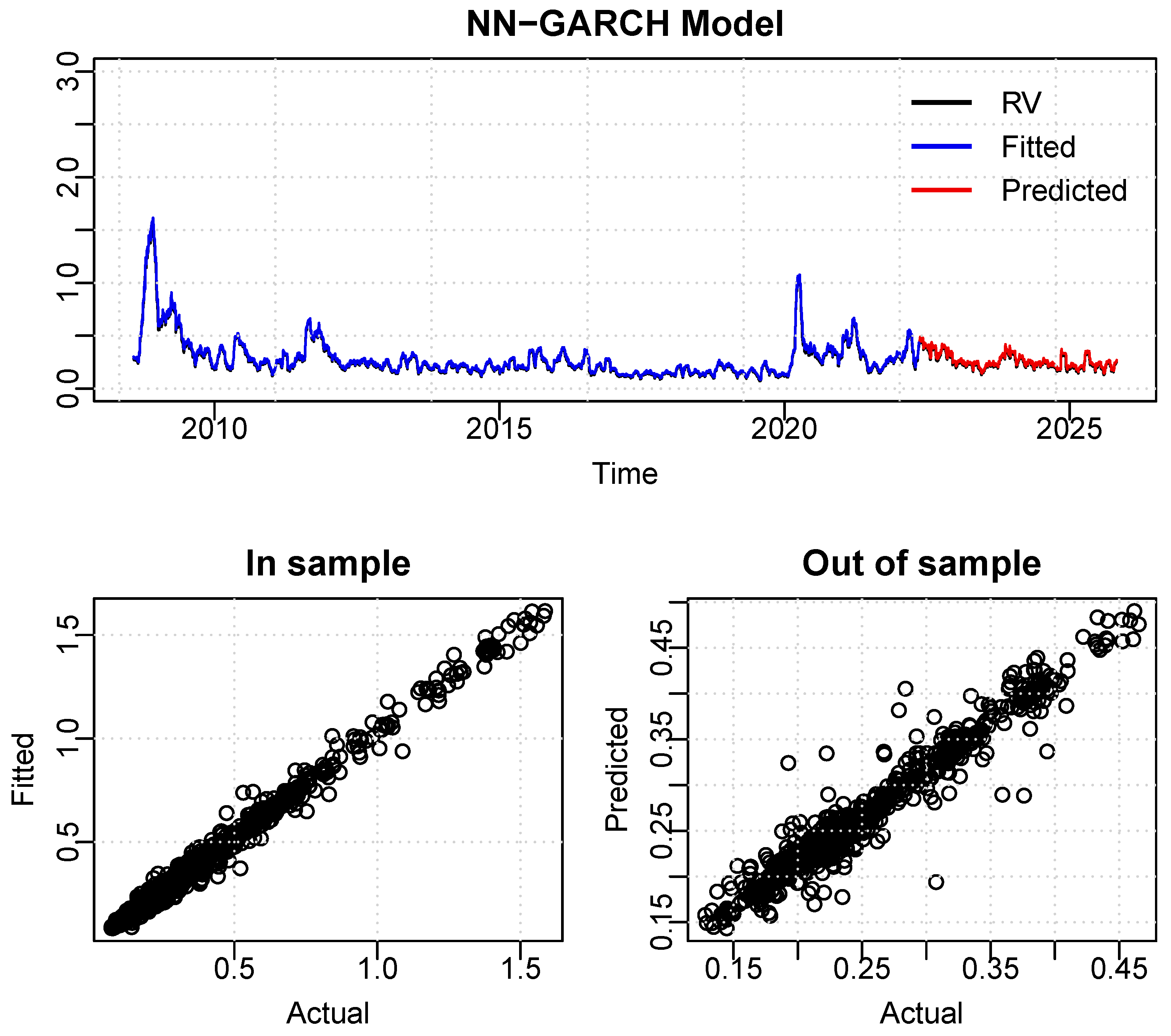
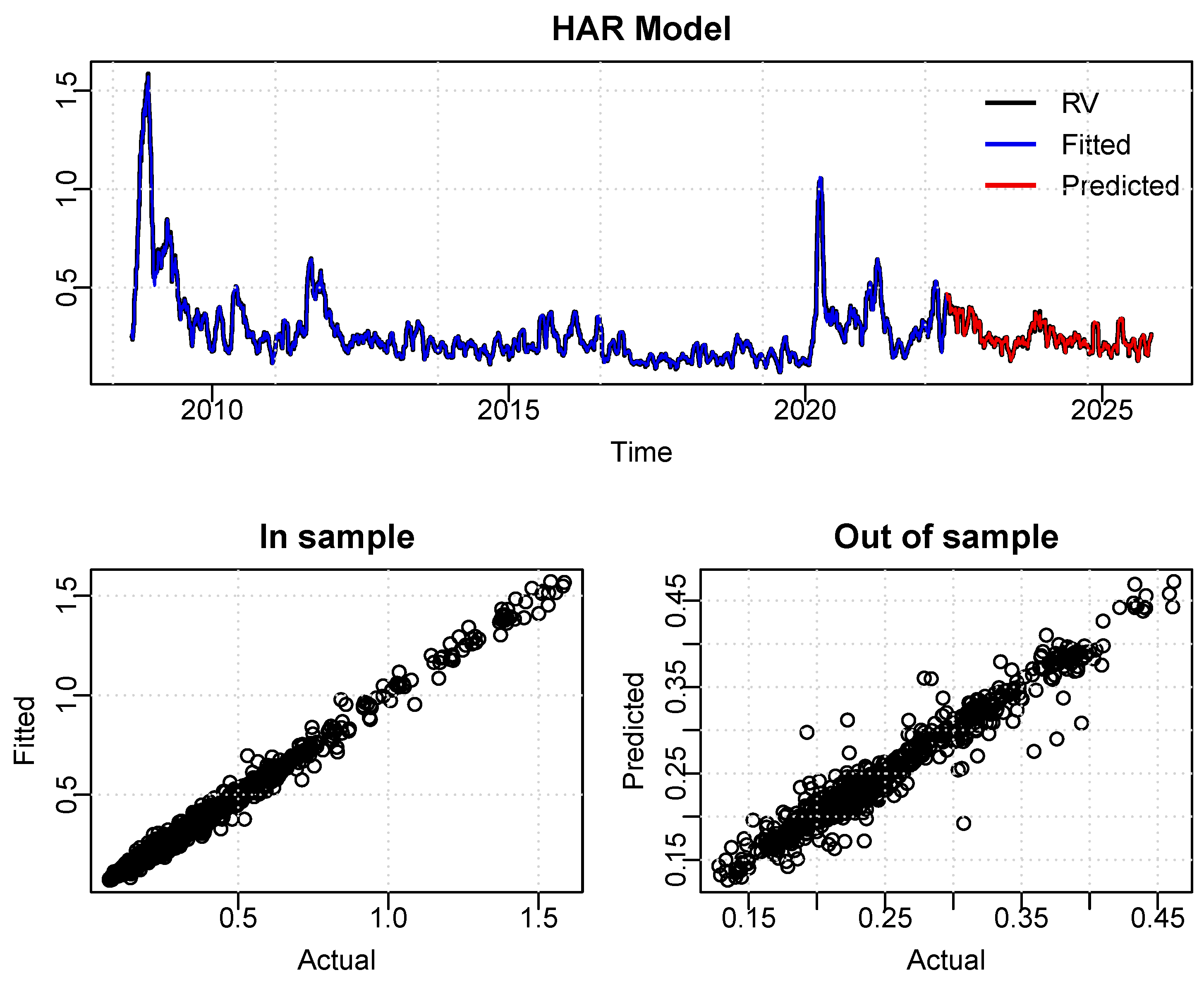
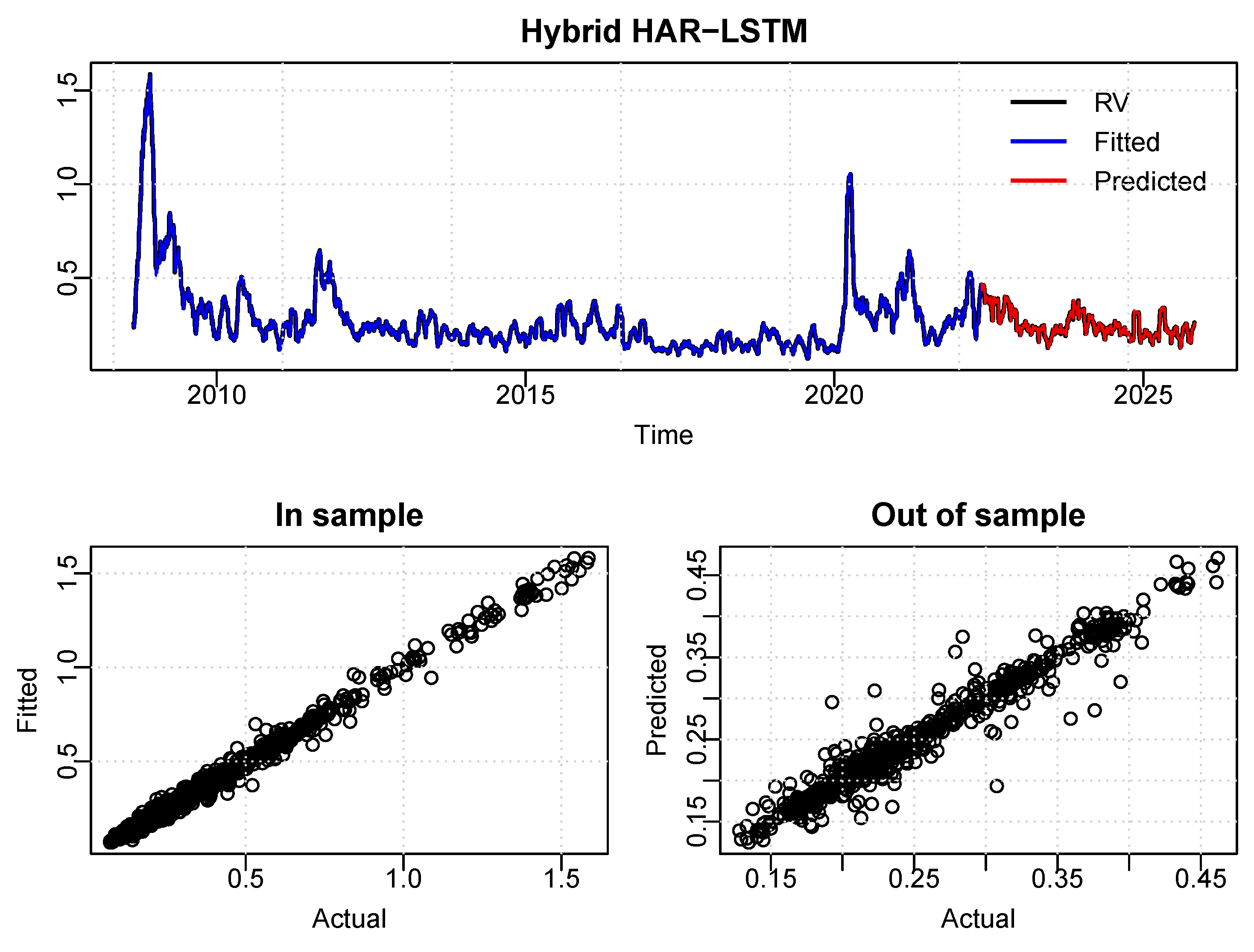
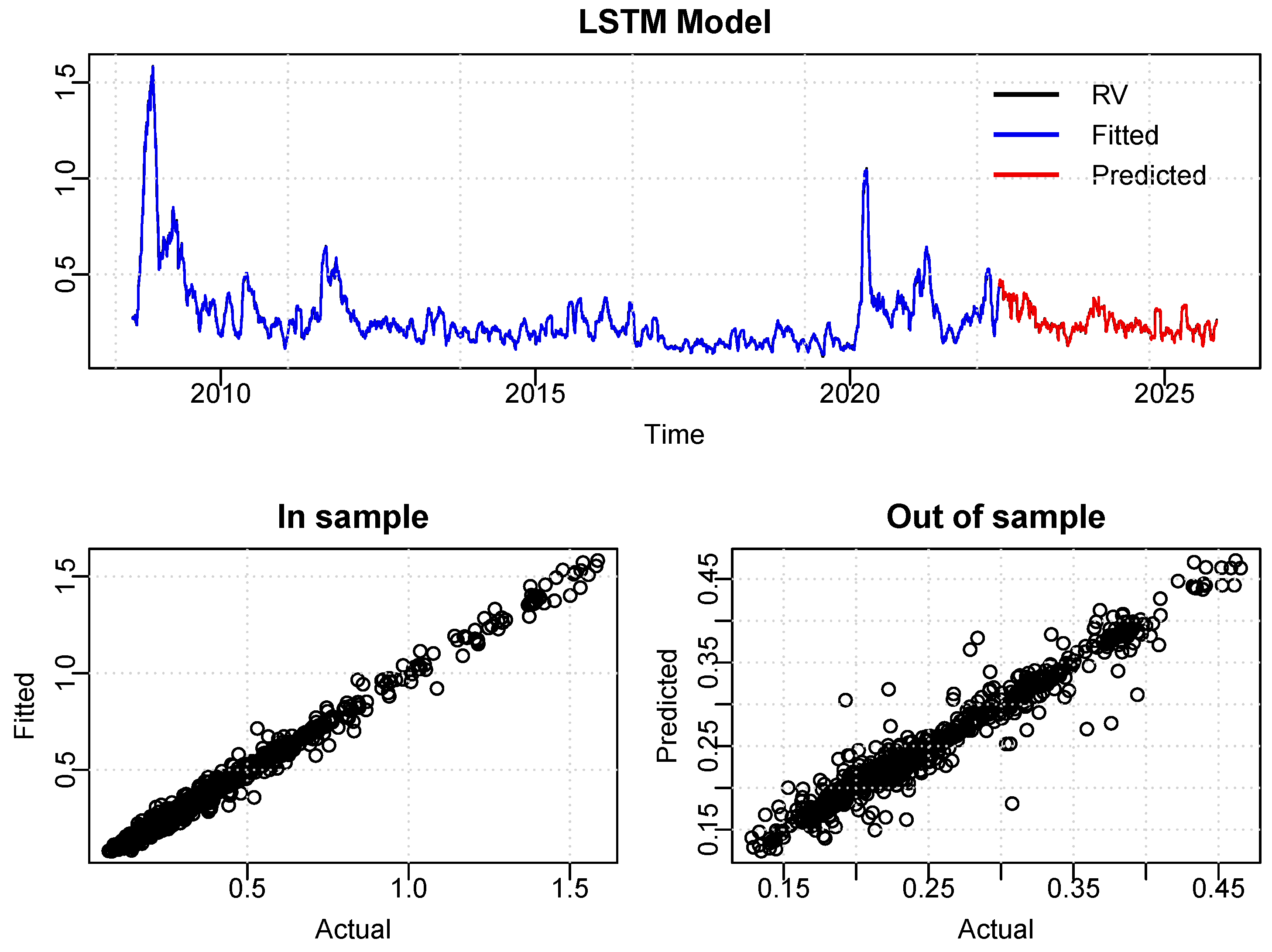
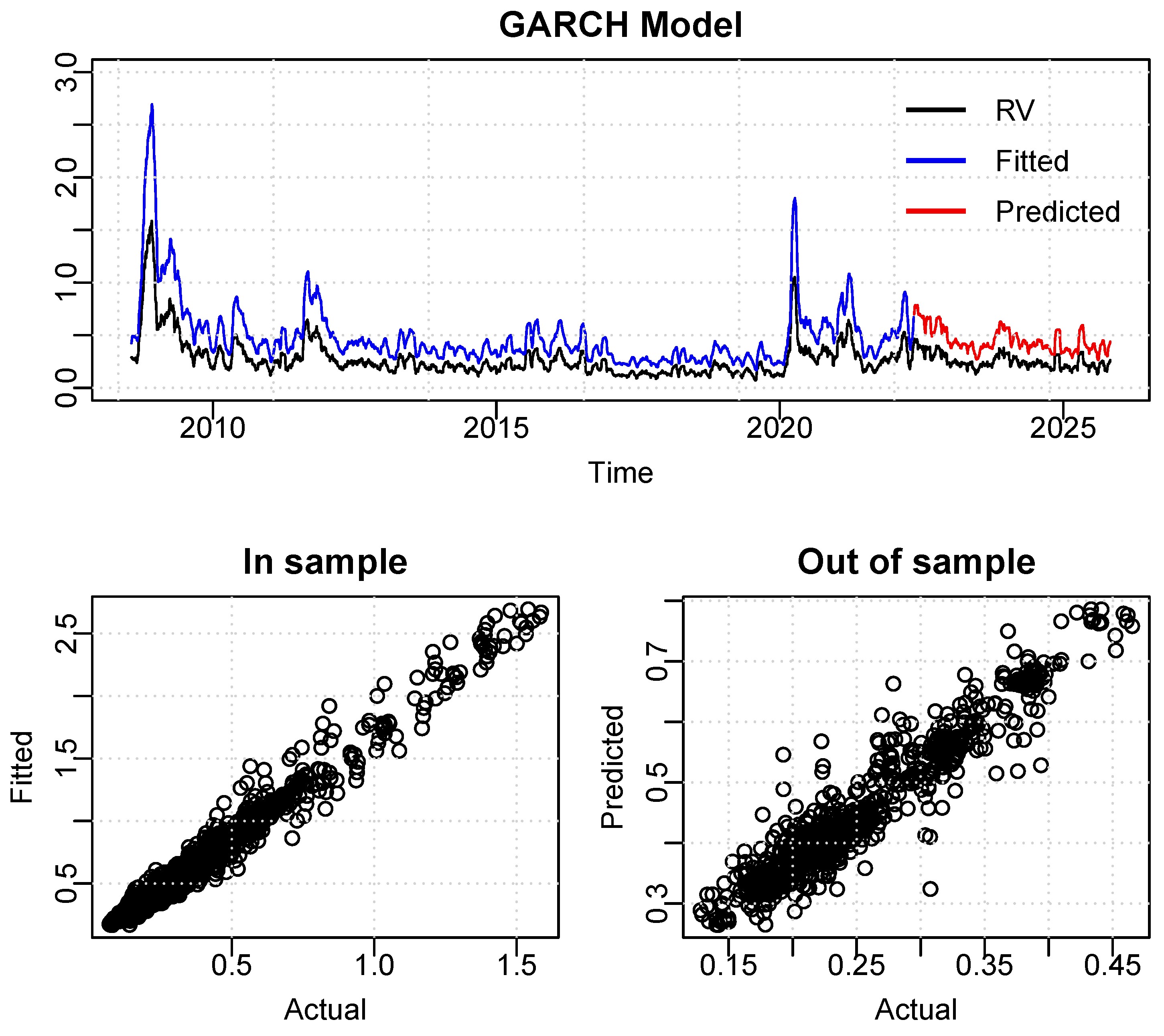
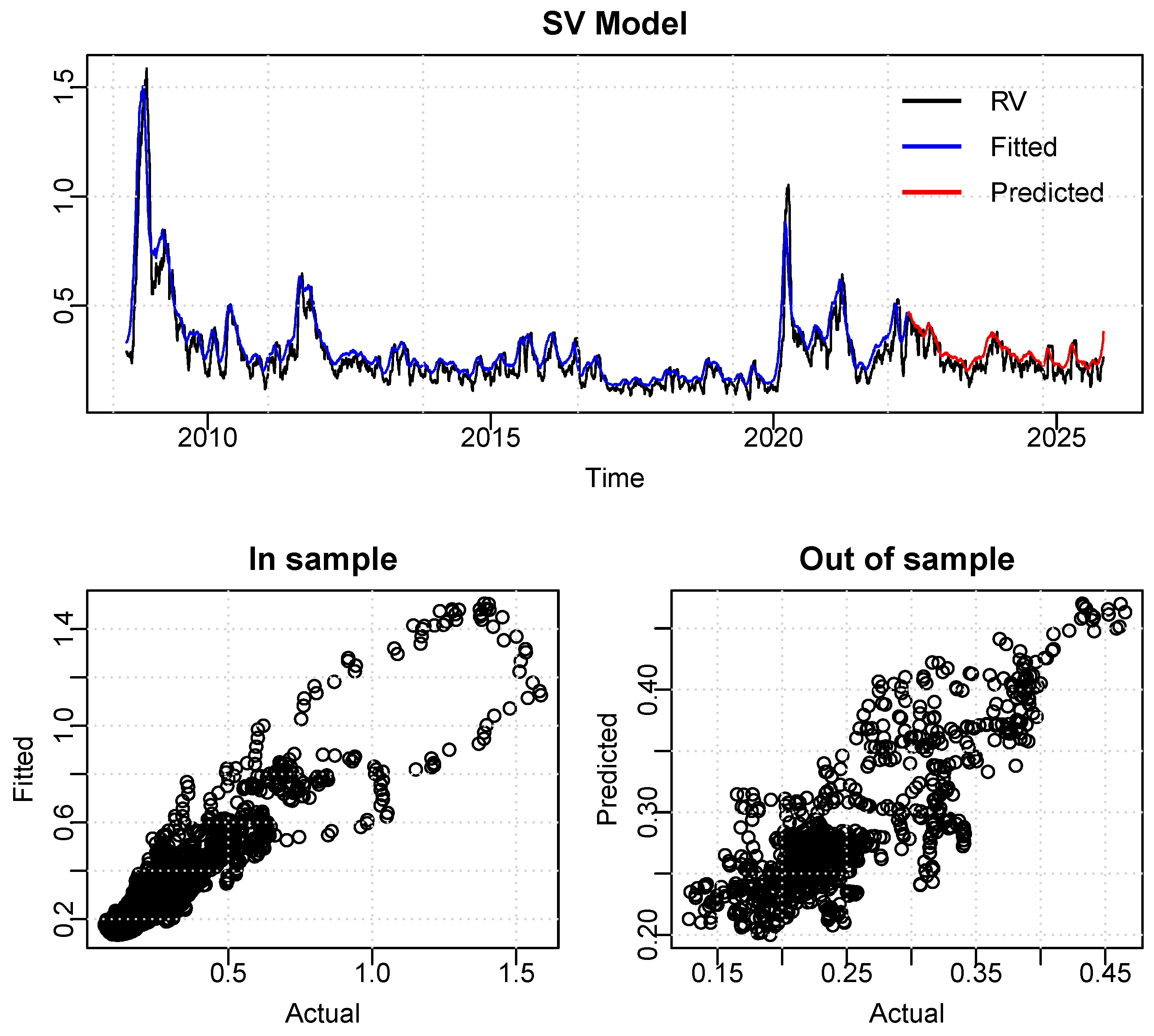
The graphical analysis (Figure 3, Figure 4, Figure 5, Figure 6, Figure 7 and Figure 8) provides compelling visual evidence of the models’ performance across different market conditions. The comparative forecast plots show that while all models generally track the direction of volatility movements, the HAR-LSTM hybrid provides a superior fit during turning points and extreme events. The LSTM alone shows some overshooting during calm periods, while the HAR model tends to under-react to sudden market movements. The SV model produces a very smooth and persistent volatility path, which fails to capture the high-frequency fluctuations and sharp spikes present in the realized volatility series. This visual evidence aligns with its poor statistical scores, demonstrating its misalignment with the characteristics of the target variable. The GARCH model struggles to capture the high-frequency components of realized volatility, consistent with its design for conditional variance rather than realized volatility forecasting.

The hybrid model’s residuals exhibit lower variance and less autocorrelation than the benchmark models, particularly during turbulent market periods. This visual evidence supports the statistical findings and demonstrates the effectiveness of the sequential modeling approach in capturing both linear persistence and non-linear dynamics.

4.4. Model Confidence Set Test

We employed the Model Confidence Set (MCS) test to statistically compare the predictive performance of all models.

Table 5. MCS test.

Model	MSE	MAE	QLIKE
HAR-LSTM	1.000	1.000	1.000
HAR	0.01132	0.000	0.01328
LSTM	0.000	0.000	0.000
SV	0.000	0.000	0.000
GARCH	0.000	0.000	0.000
GJR-GARCH	0.000	0.000	0.000
NN-GARCH	0.000	0.000	0.000

Note: MCS p-values from 25,000 bootstrap simulations using T.range statistics. Bolded values (equal to 1) identify the model(s) with the best out-of-sample forecast accuracy.

presents the MCS p-values derived from this analysis. As illustrated in Table 5, the Model Confidence Set procedure indicates that the HAR-LSTM hybrid model delivers statistically superior forecasting performance. It is the only model consistently retained in the final confidence set across all evaluated loss functions—MSE, MAE, and QLIKE—which assess different error characteristics, thereby underscoring its robust predictive ability. Conversely, the benchmark models (HAR, LSTM, SV, and GARCH) are sequentially eliminated, confirming their significantly lower accuracy.

5. Model Interpretation and Economic Significance

The superior performance of the hybrid approach can be attributed to its effective decomposition of the volatility forecasting problem. The HAR component provides a robust foundation by capturing the persistent, multi-scale volatility dynamics through its economically interpretable structure, while the optimized LSTM component (with 36 units, as determined by Bayesian optimization) focuses specifically on learning the non-linear residuals that escape linear modeling.

The 8.2% improvement in out-of-sample accuracy over the standalone LSTM demonstrates the value of this sequential approach. Rather than forcing a single model to learn both linear persistence and non-linear dynamics simultaneously, the hybrid framework allows each component to specialize in its respective domain. This specialization is reflected in the different optimal architectures identified through Bayesian optimization—the standalone LSTM requires greater capacity (97 units) to handle the full complexity of raw volatility forecasting, while the hybrid LSTM can achieve superior performance with a more focused architecture (36 units) dedicated solely to residual modeling.

From a risk management perspective, the performance improvements are economically meaningful. For energy trading portfolios and derivative positions, the enhanced forecasting accuracy translates to more precise Value-at-Risk estimates, improved option pricing, and more effective hedging strategies. The consistent outperformance across both calm and volatile periods (as visually evident in Figure 3, Figure 4, Figure 5 and Figure 6 ensures reliability across different market regimes, which is particularly valuable in the structurally unstable energy markets.

As illustrated in

Table 6. OLS Estimates of HAR model.

	Estimate	Std. Error	t Value	Pr(>|t|)
(Intercept)	0.00361	0.00051	7.06079	0.00000
RV1	0.66030	0.02259	29.22560	0.00000
RV5	0.45133	0.02546	17.72667	0.00000
RV22	−0.12439	0.00551	−22.57429	0.00000

, the results strongly suggest that the future of volatility forecasting lies not in choosing between econometric and machine learning approaches, but in developing sophisticated frameworks that leverage their complementary strengths. The HAR-LSTM hybrid represents a promising step in this direction, achieving both statistical superiority and practical utility for energy market participants.

6. Conclusions

This study has introduced and empirically validated a novel three-stage hybrid framework, the HAR-LSTM-GARCH model, for forecasting realized volatility in the complex and vital crude oil market. The model is founded on a powerful sequential decomposition principle, which strategically leverages the distinct strengths of econometric and machine learning paradigms. In the first stage, the Heterogeneous Autoregressive (HAR) model acts as a highly effective linear filter, capturing the persistent, multi-scale dynamics of volatility grounded in the Heterogeneous Market Hypothesis. This initial step provides a robust baseline forecast and, more importantly, isolates the non-linear residual component that linear models cannot explain. The second stage deploys a Long Short-Term Memory (LSTM) network, whose hyperparameters are meticulously tuned via Bayesian Optimization, specifically to learn these complex residual patterns. This focused approach allows the LSTM to operate with a more parsimonious and efficient architecture than a standalone LSTM model, demonstrating that residual modeling is a fundamentally different and more manageable task. The final stage innovatively applies a GARCH model to the residuals of the hybrid HAR-LSTM forecast, explicitly capturing the conditional heteroskedasticity that often persists in forecast errors—a “volatility of volatility” effect frequently overlooked in the literature.

The empirical results, derived from a comprehensive out-of-sample test period that included extreme market events, unequivocally demonstrate the superiority of this integrated approach. The proposed model consistently outperformed the benchmark HAR, GARCH(1,1), and standalone LSTM models across key statistical metrics like RMSE, MAE, and $R^2$. This performance gain is not merely a statistical artifact; it carries significant economic weight. For market participants—including commodity traders, risk managers, and policymakers—the enhanced forecast accuracy translates directly into more reliable Value-at-Risk calculations, improved derivative pricing, and more effective hedging strategies. The model’s robustness across both calm and turbulent regimes, as visually confirmed in the analysis, makes it a particularly valuable tool for navigating the inherent instability of energy markets. Ultimately, this research argues persuasively that the future of financial forecasting lies not in a rivalry between traditional econometrics and modern machine learning but in their thoughtful synthesis. The HAR-LSTM-GARCH model stands as a testament to this collaborative philosophy, offering a more complete, accurate, and practically useful framework for understanding and predicting risk in the global energy sector.

Despite its compelling results, this study is subject to several limitations that offer avenues for future research. Firstly, the reliance on a single asset class (Brent Crude oil) and a specific volatility measure (a proxy for Realized Volatility based on daily squared returns) may affect the generalizability of the findings. Future work should validate the model across other energy commodities (e.g., natural gas, WTI crude oil) and different financial markets, using high-frequency data to construct more precise realized volatility measures that incorporate jump components.

Secondly, the computational intensity of the framework is non-trivial. The sequential process involving HAR estimation, Bayesian optimization for the LSTM, and subsequent GARCH fitting requires significant time and resources, which may hinder its application in high-frequency trading contexts or for practitioners with limited computational capacity.

Thirdly, while the hybrid model improves forecast accuracy, it remains somewhat of a “grey box.” The HAR and GARCH components are interpretable, but the patterns learned by the LSTM in the second stage are not easily decipherable. Enhancing the model’s interpretability, for instance, by using attention mechanisms or SHAP analysis on the LSTM’s inputs, would be a valuable extension.

Finally, the model is primarily univariate, forecasting volatility based solely on its own past. It does not explicitly incorporate external fundamental or macroeconomic drivers, such as OPEC announcements, inventory data, or geopolitical risk indices, which are known to be significant drivers of oil price volatility. Integrating such exogenous variables into the hybrid framework represents a promising direction for further enhancing its predictive power and economic relevance.