Article

Maximum Entropy Identification of Latent Financing Flows in Corporate Balance Sheets: Cross-Sectoral Panel Evidence


by
Sunnatov Yusuf Usmonovich
Department of Accounting and Statistics, Bukhara State University, 11 Muhammad Iqbol Street, Bukhara 200117, Uzbekistan
J. Risk Financ. Manag. 2026, 19(6), 439; https://doi.org/10.3390/jrfm19060439
Submission received: 2 April 2026 / Revised: 7 June 2026 / Accepted: 8 June 2026 / Published: 17 June 2026
(This article belongs to the Special Issue Mathematical Modelling in Economics and Finance)

Abstract

Corporate balance sheets report aggregate equity and liability totals but conceal the internal allocation of financing sources across asset categories—an identification problem that conventional econometric methods cannot resolve without additional parametric assumptions. This paper develops a maximum entropy (ME) panel estimator to recover two latent scalar parameters: x ∈ (0,1), the share of equity capital directed toward long-term asset financing, and y ∈ (0,1), the corresponding debt allocation share. Grounded in maximum entropy principle, the estimator selects the unique parameter vector that satisfies the mean-level balance-sheet constraint while maximising joint Shannon entropy—the least-biassed solution consistent with observable data. The closed-form logistic representation yields a scalar Lagrange multiplier λ*, interpreted as a financing pressure index, recoverable via bisection in at most 21 iterations at tolerance ε = 10−5. Building on the ME estimates, we introduce a continuous matching alignment index M* = x* − y* that measures the degree of compliance with the financial matching principle along a continuous spectrum rather than as a binary categorisation. Applied to a ten-firm, cross-sectoral panel spanning Technology, Finance, Energy, and Automotive sectors over an observation window spanning 2001 to 2025 (with firm-specific subperiods reflecting differences in IPO dates and data availability), the framework reveals substantial heterogeneity in latent financing flows: equity allocation shares range from 30.1% (NVIDIA) to 75.1% (ExxonMobil), while debt allocation shares span 37.1% to 77.5%. Across the panel, only Meta exhibits substantial positive matching alignment, while Microsoft, ExxonMobil, Apple, and Tesla show only very slight differences that fall within the neutral band, and the remaining firms show varying degrees of structural departure from the matching benchmark; the thresholds used to summarise these descriptive labels are interpretive aids rather than re-imposed binary criteria, and the substantive ranking of firms along M* does not depend on the specific threshold values adopted. The ME solution’s entropy H(x*, y*) and the normalised diversification index D(x*, y*) describe allocation balance under the estimator’s information–theoretic criterion rather than independently observed firm complexity; in the present sample, the cross-firm ordering of these values is not recovered by firm size, leverage, or sector classification alone. These findings, based on a ten-firm case-study panel with time-invariant allocation parameters, should be interpreted as descriptive patterns of the present sample rather than statistically validated regularities. They provide a theoretically rigorous and computationally tractable identification of unobservable corporate financing flows, with potential implications for capital structure theory, financial risk assessment, and balance sheet analysis that would benefit from validation on larger and more representative samples in future work.

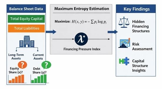
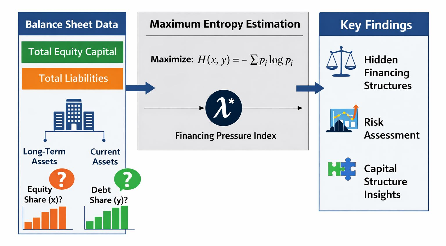
Graphical Abstract

1. Introduction

The allocation of financing sources across asset categories constitutes one of the most consequential yet empirically elusive dimensions of corporate financial policy. Standard financial statements, prepared under U.S. GAAP or IFRS, disclose aggregate totals of equity capital and total liabilities alongside aggregate asset categories—yet remain silent on the internal mapping between financing instruments and asset classes. This informational gap is not merely an accounting artefact: it represents a fundamental identification problem that precludes direct empirical testing of foundational capital structure propositions, including the financial matching principle (Morris, 1976), the hedging hypothesis (Myers, 1977), and asset–liability duration alignment theories (Hart & Moore, 1994). Without knowledge of how equity and debt are internally allocated across long-term and current assets, empirical capital structure research is constrained to observable leverage ratios and aggregate financing totals—proxies that conflate structurally distinct financing configurations.
The consequences of this identification gap are economically significant. Two firms with identical debt-to-equity ratios may direct their financing toward structurally distinct asset configurations—yet conventional leverage metrics assign them the same capital structure characterisation. This observational equivalence problem has been acknowledged in the theoretical literature (Titman & Wessels, 1988; Rajan & Zingales, 1995; Frank & Goyal, 2009) but has resisted empirical resolution due to the absence of a tractable identification framework. Existing approaches—supplementary disclosures, parametric structural models, and reduced-form empirical strategies—each carry significant limitations: they are either data-intensive and non-replicable at scale, impose untestable distributional assumptions, or sacrifice structural interpretability entirely (Barclay & Smith, 1995; Welch, 2004; Graham & Leary, 2011).
This paper introduces a maximum entropy (ME) panel estimator that resolves the financing allocation identification problem without imposing parametric assumptions beyond the balance-sheet identity itself. The approach applies the maximum entropy principle of Jaynes (1957)—the canonical resolution of ill-posed inverse problems under incomplete information—to recover two latent scalar parameters: x ∈ (0,1), representing the share of equity capital directed toward long-term asset financing, and y ∈ (0,1), the corresponding debt liability allocation share. The estimator selects the unique parameter vector that satisfies the mean-level balance-sheet constraint while maximising joint Shannon entropy—yielding, in the precise sense of Jaynes (1957), the least-biassed solution consistent with observable aggregate data. The resulting closed-form logistic representation is computationally tractable, guaranteeing interior solutions and convergence within 21 bisection iterations at tolerance ε = 10−5. Crucially, the Lagrange multiplier associated with the binding constraint admits direct economic interpretation as a financing pressure index—a cardinal measure of the departure from a neutral 50/50 allocation between asset categories.
Building on the ME estimates, the paper develops a continuous matching alignment index M* = x* − y* that captures, on a single scalar dimension, the degree to which a firm’s equity allocation to long-term assets exceeds (or falls short of) its debt allocation to the same category. Because M* is a difference in two interior logistic-form quantities, it is itself uniquely determined by the ME solution and admits a direct economic interpretation: M* > 0 indicates that equity is the dominant long-term financing source relative to debt (alignment with the matching principle), while M* < 0 indicates the opposite. This formulation supersedes the binary x* > 0.5 ∧ y* < 0.5 classification used in earlier ME-style analyses, which—as shown in Section 3.6—imposes mutually inconsistent sign restrictions on λ* and is therefore not satisfiable in the single-multiplier ME framework. The continuous index avoids that internal inconsistency and yields a finer-grained ordering of firms along the matching dimension.
The framework is applied to a ten-firm, cross-sectoral panel spanning Technology, Finance, Energy, and Automotive sectors over an observation window covering 2001 to 2025 (with firm-specific subperiods reflecting IPO dates and data availability) and encompassing two major systemic disruptions: the Global Financial Crisis of 2008–2009 and the COVID-19 shock of 2020. This multi-sector, long-horizon design enables three distinct empirical contributions. First, it reveals substantial cross-firm heterogeneity in latent financing flows that is entirely undetectable from conventional leverage metrics. Second, it provides the first systematic empirical assessment of matching principle alignment across sectors using balance-sheet-consistent allocation parameters and the continuous M* index. Third, it demonstrates that the ME solution’s entropy H(x*, y*) and normalised diversification index D(x*, y*)—interpreted as descriptors of allocation balance under the estimator’s information–theoretic criterion rather than independent measures of firm complexity—order firms in ways that conventional firm size and leverage metrics cannot recover, challenging the implicit assumption in much of the empirical capital structure literature that observable financing ratios are sufficient statistics for financing structure.
The empirical results, summarised through the continuous matching alignment index, indicate that only one firm in the sample—Meta—exhibits substantial positive matching alignment. Microsoft shows only a very slight positive difference that falls within the neutral band; ExxonMobil, Apple, and Tesla are also essentially neutral, and the remaining firms—Alphabet, Amazon, NVIDIA, Toyota, and JPMorgan—show progressively stronger negative alignment, with JPMorgan exhibiting the most pronounced structural departure. The verbal labels used here (“substantial,” “marginal,” “neutral,” “moderate,” “strong negative”) summarise five interpretive bands defined in Section 3.6; we emphasise that they are presentational aids derived from the continuous M* index, not a re-imposed binary classification. Firms in capital-intensive sectors—ExxonMobil, Toyota, and JPMorgan—exhibit high allocation shares in both dimensions, reflecting infrastructure co-financing requirements that conventional leverage analysis conflates with overleveraging. NVIDIA’s near-zero leverage translates into an equity-constrained allocation (x* = 30.1%) inconsistent with matching alignment, despite its conservative financing reputation. Apple’s sustained share-repurchase programme has steeply eroded its book equity—which declined by roughly 60% from its 2017 peak while remaining positive—and although Apple’s proportional allocation shares fall within the neutral band at the panel-mean level, in absolute dollar terms debt remains the dominant long-term financing instrument—a finding with direct implications for financial risk assessment.
This paper makes three contributions to the capital structure literature. Methodologically, it introduces the first maximum entropy panel estimator for latent financing flow identification, providing a theoretically grounded and computationally tractable alternative to parametric structural models, together with a continuous matching alignment index derived from the ME estimates. Empirically, it delivers the first systematic cross-sectoral decomposition of unobservable equity and debt allocation shares using standard balance-sheet data across a panel spanning up to 25 years. Theoretically, it operationalises a cardinal financing pressure index derived from the Lagrange multiplier of the entropy-maximisation problem, and links it analytically to the matching alignment index, offering a new tool for the empirical assessment of asset–liability matching alignment. Taken together, these contributions extend the empirical frontier of capital structure research by making the latent financing allocation mechanism directly observable.
The remainder of the paper is organised as follows. Section 2 reviews the relevant literature on capital structure, asset–liability matching, and entropy-based methods in finance. Section 3 develops the maximum entropy estimator, establishes its theoretical properties, derives the bisection algorithm, and introduces the matching alignment index. Section 4 presents descriptive statistics, ME estimation results, matching alignment analysis, and financing archetype classification. Section 5 concludes with implications for capital structure theory and directions for future research.

2. Literature Review

2.1. Capital Structure Theory: Foundations and Competing Frameworks

The theoretical foundations of capital structure analysis rest on the landmark irrelevance propositions of Modigliani and Miller (1958, 1963), who demonstrated that, absent taxes and frictions, the market value of a firm is independent of its financing mix. This canonical benchmark established the logical starting point for subsequent inquiry by clarifying that observed financing heterogeneity must originate from market imperfections, including corporate taxation, financial distress costs, information asymmetries, and agency conflicts. The introduction of the tax shield benefit of debt in Modigliani and Miller (1963) generated the first structural motive for leverage, setting the stage for what would become known as the trade-off theory of capital structure.
The static trade-off theory, formalised by Kraus and Litzenberger (1973) and extended by Scott (1976), posits that firms select an optimal leverage ratio by balancing the marginal tax benefit of debt against the marginal expected cost of financial distress. A rich empirical literature has tested this proposition, with mixed results. Frank and Goyal (2009) document that observable firm characteristics—profitability, asset tangibility, size, and industry classification—explain a substantial fraction of cross-sectional leverage variation, consistent with trade-off theory predictions. However, Welch (2004) and Lemmon et al. (2008) demonstrate that firm fixed effects dominate observed capital structure, with leverage ratios exhibiting remarkable time-series persistence that conventional trade-off factors cannot account for. The implication is that unobservable, firm-specific financing policies constitute the primary determinant of capital structure—an insight directly motivating the latent parameter identification approach developed in the present study.
Myers (1984) and Myers and Majluf (1984) proposed an alternative paradigm, the pecking order theory, grounded in adverse selection costs under asymmetric information between managers and outside investors. The pecking order predicts that firms prefer internal financing to debt and debt to equity, generating a financing hierarchy that precludes the existence of a well-defined target leverage ratio. Empirical support for the pecking order has been documented by Shyam-Sunder and Myers (1999), who find that a financing deficit model significantly outperforms a target-adjustment specification for large U.S. firms. However, Frank and Goyal (2003) show that pecking order predictions fail for small, high-growth firms, where information asymmetry is arguably most severe. More recently, Fama and French (2005) document that equity issuance is far more frequent than the pecking order predicts, casting doubt on its universality.
Market timing theory, advanced by Baker and Wurgler (2002), proposes that capital structure evolves as the cumulative outcome of managers’ attempts to exploit equity market mispricing, issuing equity when valuations are high and repurchasing when low. Baker and Wurgler (2002) find that historical market-to-book ratios have persistent effects on leverage, consistent with market timing rather than dynamic adjustment toward a target. The share-repurchase phenomenon documented in the present study—particularly Apple’s sustained equity depletion through buybacks exceeding $600 billion since 2012—represents an extreme manifestation of market timing effects on balance-sheet structure that aggregate leverage metrics systematically mischaracterise.
A significant development in the empirical capital structure literature concerns the role of firm heterogeneity and unobservable factors. Lemmon et al. (2008) decompose capital structure into a persistent, firm-specific component and a transitory, time-varying component, finding that the former accounts for the majority of observed leverage variation. Graham and Leary (2011) and Faulkender et al. (2012) document that adjustment toward target leverage is slow and costly, implying that observed leverage ratios are poor proxies for desired financing structures at any given point in time. These findings underscore the insufficiency of observable leverage ratios as representations of underlying financing policy—the fundamental motivating observation of the present paper.

2.2. The Identification Problem in Capital Structure Research

The empirical capital structure literature confronts a fundamental identification problem: standard financial statements, prepared under U.S. GAAP or IFRS, disclose aggregate totals of equity capital and total liabilities alongside aggregate asset categories, but remain silent on the internal mapping between financing instruments and asset classes. This informational gap is not merely an accounting artefact—it represents a structural constraint that precludes direct empirical testing of foundational capital structure propositions, including asset–liability matching (Morris, 1976), the hedging hypothesis (Myers, 1977), and duration alignment theories (Hart & Moore, 1994).
The consequences of this identification gap are economically non-trivial. Titman and Wessels (1988) acknowledge that standard leverage ratios conflate structurally distinct financing configurations, noting that asset tangibility and uniqueness differentially affect the composition of financing sources in ways that aggregate measures cannot disentangle. Rajan and Zingales (1995) demonstrate that even the choice between book-value and market-value leverage introduces systematic measurement error, depending on whether one wishes to capture the firm’s historical financing decisions or its current obligations relative to market value. Harris and Raviv (1991), in their influential survey, explicitly identify the absence of micro-level financing allocation data as a binding constraint on the testability of capital structure theory.
Three broad empirical strategies have been employed to address this identification challenge. The first relies on supplementary disclosures—debt maturity schedules, asset footnotes, and segment reporting—to infer partial allocation information. Barclay and Smith (1995) and Stohs and Mauer (1996) exploit debt maturity data to test matching principle predictions, finding partial support for duration alignment. This approach is data-intensive, sample-restricted to firms with detailed footnote disclosures, and non-replicable across standard financial databases such as Compustat, which record only aggregate totals. Rauh and Sufi (2010) provide a notable exception, constructing firm-level debt structure measures from SEC filings to document that most firms maintain heterogeneous debt portfolios combining secured and unsecured, short-term and long-term instruments. Their findings highlight that aggregate leverage conceals structurally important within-firm variation—a problem analogous to, though distinct from, the equity-versus-debt allocation problem addressed in the present study.
The second strategy employs structural models that impose parametric assumptions on the financing–asset relationship. Dynamic capital structure models, including those of Fischer et al. (1989) and Goldstein et al. (2001), derive optimal leverage policies under specific distributional assumptions about asset value processes and tax treatment. While these models generate internally consistent financing predictions, their identifying assumptions—regarding, for example, the geometric Brownian motion of asset values or the linearity of distress costs—are untestable by construction and may introduce systematic bias. Welch (2004) demonstrates that capital structure models with plausible parameter values generate leverage predictions that are quantitatively inconsistent with observed corporate behaviour, suggesting that structural assumptions routinely employed in the literature are empirically untenable.
The third approach, predominant in recent reduced-form empirical work, sidesteps the allocation problem entirely by focusing on associations between observable financing ratios and firm characteristics (Graham & Leary, 2011; Faulkender et al., 2012). While tractable, this strategy sacrifices structural interpretability in exchange for empirical convenience, leaving the latent allocation mechanism unidentified. The present paper introduces a maximum entropy panel estimator that resolves the financing allocation identification problem without imposing parametric assumptions beyond the balance-sheet identity—occupying a methodological position between the supplementary-disclosure approach (which requires data unavailable at scale) and the structural modelling approach (which imposes distributional assumptions that are fundamentally untestable).

2.3. Asset–Liability Matching and the Financial Hedging Hypothesis

The financial matching principle, articulated by Morris (1976) and extended by Myers (1977) in the context of the debt overhang problem, prescribes that firms should align the duration of their liabilities with the duration of the assets those liabilities finance. The intuition is straightforward: financing long-term, illiquid assets with short-term debt exposes firms to liquidity risk (the inability to refinance at maturity) and rollover risk (refinancing at adverse rates), while financing short-term assets with long-term debt imposes unnecessary interest costs and inflexibility. The matching principle thus constitutes a normative benchmark for financing policy that carries direct implications for financial risk, default probability, and firm value.
Hart and Moore (1994) provide a theoretical foundation for maturity matching in a model where long-term debt constrains managerial discretion and mitigates the hold-up problem between firms and their creditors. Their framework predicts that asset duration should determine debt maturity in equilibrium—a prediction tested empirically by Barclay and Smith (1995) and Guedes and Opler (1996). Both studies find partial support for the matching hypothesis using proxies for asset duration, but the absence of direct allocation data forces reliance on indirect measures (book-to-market ratios, earnings volatility) that conflate asset duration with other firm characteristics.
Almeida and Campello (2007) and Acharya et al. (2007) extend the matching literature by demonstrating that financially constrained firms face a trade-off between hedging future investment needs and financing current operations, generating endogenous departures from the matching principle that depend on the correlation between asset cash flows and financing opportunities. Their theoretical predictions imply that matching alignment should be more prevalent among unconstrained firms with stable, predictable cash flows—a prediction broadly consistent with the present study’s finding that strong matching alignment is confined to firms with substantial internal cash generation and minimal financial constraints. Departures from alignment among capital-intensive firms reflect structural co-financing requirements rather than sub-optimal financing policy, a distinction that aggregate leverage metrics cannot draw.
The empirical assessment of matching alignment has been further complicated by the introduction of complex financial instruments that blur the asset–liability duration relationship. Interest rate swaps, cross-currency swaps, and other derivatives allow firms to separate the economic duration of their liabilities from their contractual maturity (Chernenko & Faulkender, 2012; Campello et al., 2011). Faulkender (2005) documents that firms use interest rate swaps to actively manage the duration exposure of their balance sheets, implying that observable debt maturity is an imperfect proxy for economic liability duration. In the context of the present study, this observation reinforces the need for a balance-sheet-consistent identification approach that does not rely on derivatives disclosures or debt maturity schedules unavailable in standard financial databases.

2.4. Entropy Methods in Finance: From Portfolio Theory to Capital Structure

The application of information–theoretic entropy measures to financial problems has a long history, originating in Philippatos and Wilson’s (1972) seminal application of Shannon entropy to portfolio selection. Shannon (1948) defined information entropy as the measure of uncertainty associated with a probability distribution, and Jaynes (1957) established the maximum entropy principle as the canonical method for recovering the least-biassed probability distribution consistent with a finite set of observable constraints. The present study applies the Jaynes (1957) framework to the capital structure identification problem, recovering the unique parameter vector that satisfies the mean-level balance-sheet constraint while maximising joint Shannon entropy.
In the portfolio selection context, entropy-based approaches have been motivated by the inadequacy of variance as a risk measure for non-normal return distributions and by the tendency of mean–variance optimisation to generate poorly diversified, estimation-sensitive portfolios. Usta and Kantar (2011) and DeMiguel et al. (2009) demonstrate that entropy-based portfolio rules achieve out-of-sample Sharpe ratios comparable to or exceeding sophisticated mean–variance strategies, providing empirical support for the view that entropy maximisation is a robust objective under uncertainty. More recently, Mercurio et al. (2020) applied maximum entropy methods to construct sparse, diversified portfolios under transaction cost constraints, demonstrating computational tractability in high-dimensional problems.
In the asset pricing context, maximum entropy methods have been used to recover risk-neutral probability distributions from observed option prices (Buchen & Kelly, 1996; Stutzer, 1996; Avellaneda et al., 1997). This literature exploits the duality between entropy maximisation and minimum-cost pricing in incomplete markets, using observable option prices as moment constraints and the maximum entropy distribution as the least informative risk-neutral measure consistent with market data. The structural analogy to the present study is direct: both applications use the maximum entropy principle to recover a latent distribution (risk-neutral probabilities; financing allocation parameters) from observable aggregate quantities (option prices; balance-sheet totals) under incomplete information.
Recent contributions have extended entropy methods to capital markets microstructure and systemic risk analysis. Bowden (2011) proposes entropy-based measures of market information flow, while Cabrales et al. (2017) apply entropy concepts to characterise the resilience of financial networks. In the corporate finance context, Golan et al. (1996) develop generalised maximum entropy estimators for ill-posed inverse problems in economics, providing the methodological foundation for the present study’s panel estimation approach. Their framework demonstrates that maximum entropy estimation produces consistent and asymptotically normal estimates under mild regularity conditions, and that the associated Lagrange multipliers have direct economic interpretations as shadow prices of the binding constraints—a property exploited in the present study’s construction of the financing pressure index λ* and the matching alignment index M*.
The specific application of entropy methods to balance-sheet analysis is, to the best of our knowledge, novel. The closest antecedents are the entropy-based decomposition methods applied to input–output analysis (Golan et al., 1996) and the maximum entropy estimation of trade flows in international economics (Bacchetta et al., 2012). We cite Bacchetta et al. (2012) specifically for the methodological analogy it offers to the present problem—recovering a latent allocation matrix from observable row and column margins—rather than for its substantive trade-policy content. In both cases, the maximum entropy principle is invoked to recover a latent allocation matrix from observable aggregate row and column sums—a problem structurally identical to the one solved in the present paper, where the aggregate row sum is total long-term assets and the column sums are total equity and total debt.

2.5. Debt Maturity Structure and Cross-Sectoral Financing Heterogeneity

The substantial empirical literature has examined the determinants of corporate debt maturity as a proxy for the asset–liability duration relationship. Barclay and Smith (1995) find that regulated firms and those with high-growth opportunities favour shorter debt maturities, while Stohs and Mauer (1996) document a positive but modest association between asset maturity and debt maturity. Billett et al. (2007) show that shorter maturities and tighter covenants serve as substitutes for equity monitoring in high-agency-cost firms.
The cross-sectoral dimensions of financing heterogeneity documented in the present study have antecedents in the industry-level capital structure literature. MacKay and Phillips (2005) demonstrate that capital structure choice is strongly influenced by competitive dynamics within industries, with firms in capital-intensive sectors maintaining systematically higher leverage than those in asset-light sectors. Bradley et al. (1984) document that industry fixed effects explain a substantial fraction of leverage variation, a finding subsequently confirmed by Titman and Wessels (1988) and Graham et al. (2002). The present study extends this literature methodologically by decomposing industry-level financing heterogeneity into equity allocation and debt allocation components, and in the present case sample illustrates that the capital-intensive sector representatives (Energy, Automotive, Finance) exhibit high-allocation shares in both dimensions, suggesting co-financing structures that conventional leverage analysis would tend to conflate with overleveraging; a systematic sectoral test would require a broader cross-section of firms within each sector than the present panel provides. For the financial sector specifically, Adrian and Shin (2010) and Gropp and Heider (2010) document that banking firms exhibit extreme leverage driven by regulatory requirements and intermediation business models, and JPMorgan’s persistent c/d below 0.15 in the sample is consistent with the same regulatory-capital-driven pattern; we cite these references descriptively rather than as evidence that the single bank in our panel represents banking-sector financing structure more broadly.

2.6. Share Repurchases, Equity Depletion, and Capital Structure Dynamics

The phenomenon of equity depletion through share repurchases has emerged as a defining feature of U.S. corporate finance, with aggregate buybacks exceeding dividend payments in most years since 2004 (Fama & French, 2001). Brav et al. (2005) document that managers treat buybacks as a flexible substitute for dividends, with capital structure implications treated as secondary. Apple’s trajectory represents one of the most extreme documented cases: since initiating its buyback programme in 2012, the firm has returned over $600 billion to shareholders, and its book equity has declined steeply—by roughly 60% from its 2017 peak of approximately $134 billion to a trough of approximately $51 billion in 2022—while remaining positive; the retained earnings component of equity turned negative beginning in 2022, as cumulative repurchases and distributions exceeded accumulated profits. We emphasise that the relevant phenomenon is this severe erosion of the equity base, which makes ratio-based leverage metrics increasingly unstable and difficult to compare over time, even though they remain formally defined. Kahle and Stulz (2017) note that, in the limiting case of negative book equity—a configuration documented for several large U.S. repurchasers—conventional leverage ratios become undefined or economically uninterpretable. The present study’s ME estimation framework is robust to severe equity depletion, including the negative-book-equity limit, because it operates on absolute dollar values rather than ratios—a methodological advantage illustrated by the Apple case. We note that the time-invariance assumption on (x, y) adopted in our framework (Section 3.2.2) does not preclude an interpretation of Apple’s static (x*, y*) configuration as the time-averaged outcome of dynamic processes such as sustained share repurchases: the ME estimator recovers a single, time-invariant pair (x*, y*) that best satisfies the mean-level balance-sheet identity over the observation window, and that mean-level configuration is itself shaped by the dynamic trajectory of the underlying balance-sheet items. We emphasise that the static (x*, y*) does not, and cannot, identify the values of (x, y) in any specific subperiod (such as a pre-2012 versus post-2012 partition for Apple); it identifies only the single time-invariant pair that best reconciles the panel-mean balance-sheet quantities. Statements elsewhere in the manuscript that link Apple’s static (x*, y*) configuration to its sustained share-repurchase programme are therefore mechanism-of-influence interpretations—the post-2012 repurchase trajectory shifted the panel-mean equity downward and so shifted Apple’s time-averaged x* downward—and not claims about the values of (x, y) within the post-2012 subperiod itself. Tracing year-by-year changes in (x, y) would require relaxing the time-invariance assumption (a direction we identify for future work in Section 5); the static result reported here characterises the time-averaged outcome of those dynamic processes. More broadly, Lazonick (2014) documents that sustained buyback programmes generate systematic balance-sheet hollowing that reduces resilience to adverse shocks, a concern operationalised here through the ME decomposition of financing flows.

2.7. Positioning of the Present Study

The present paper contributes to the intersection of three distinct studies: the empirical capital structure literature, the asset–liability matching literature, and the entropy-based estimation literature. From the capital structure literature, it inherits the motivating observation that observable financing ratios are insufficient statistics for the underlying financing structure (Lemmon et al., 2008; Frank & Goyal, 2009) and the recognition that latent, firm-specific financing policies constitute the dominant driver of observed leverage heterogeneity. From the matching literature, it inherits the theoretical framework of the financial matching principle (Morris, 1976; Myers, 1977) and the empirical challenge of testing matching alignment without direct observation of financing allocation. From the entropy literature, it inherits the methodological toolkit of Jaynes’s (1957) maximum entropy estimation, Golan et al.’s (1996) generalised entropy estimation, and the growing body of entropy applications in finance (Philippatos & Wilson, 1972; Stutzer, 1996; Usta & Kantar, 2011).
The study’s primary methodological contribution is the introduction of a balance-sheet-consistent maximum entropy panel estimator that resolves the financing allocation identification problem without supplementary data or parametric structural assumptions. By maximising joint Shannon entropy subject to the mean-level balance-sheet constraint, the estimator recovers the unique interior solution (x*, y*) that is, in the precise sense of Jaynes (1957), the least biassed estimate of financing allocation consistent with observable aggregate data. The associated Lagrange multiplier λ* provides a cardinal financing pressure index that admits direct economic interpretation through the envelope theorem, and the continuous matching alignment index M* = x* − y* provides a finely graded measure of structural compliance with the matching principle. Together, these tools offer a new diagnostic apparatus for capital structure analysis that complements and in some cases contradicts conventional leverage-based risk metrics.
Empirically, the study provides the first systematic cross-sectoral decomposition of equity and debt allocation shares using standard balance-sheet data across a panel spanning up to 25 years, encompassing two major systemic disruptions. The resulting evidence—that strong matching alignment is exhibited by only one firm in the sample (Meta), with no firm in the marginal band and the next-closest firm (Microsoft) lying within the neutral band, alongside ExxonMobil, Apple, and Tesla—challenges the implicit assumption in textbook capital structure discussions that the matching principle represents a widely achievable benchmark. The demonstration that the ME solution’s entropy H(x*, y*)—interpreted as a descriptor of allocation balance under the estimator’s information–theoretic criterion rather than an independent measure of firm complexity—orders firms in ways that firm size and leverage do not recover challenges the sufficiency of observable financing ratios as descriptors of corporate financing structure, opening new empirical directions in capital structure research that move beyond leverage ratios toward the structural anatomy of corporate financing.

3. Methodology

3.1. Conceptual Foundation

Corporate balance sheets report aggregate totals of assets and financing sources but do not disclose how individual financing instruments are internally allocated across asset categories. Specifically, standard financial statements reveal the total equity capital c and total debt liabilities d, but not the shares of these sources that finance long-term assets a versus current assets b. Recovering these latent allocation shares from observable aggregate data constitutes an inherently ill-posed inverse problem: the system of balance sheet equations contains fewer binding constraints than unknowns, leaving the solution set infinite-dimensional.
The maximum entropy (ME) principle, introduced by Jaynes (1957) as an extension of Boltzmann’s statistical entropy to problems of inference under incomplete information, provides the theoretically canonical resolution of such ill-posed inverse problems. The principle selects the unique probability distribution—or, in the present context, the unique parameter vector—that satisfies all observable constraints while maximising the Shannon information entropy of the solution. This selection criterion is epistemologically equivalent to making no additional assumptions beyond what the data directly impose: the ME solution is, in a precise mathematical sense, the least biassed estimate consistent with the observed constraints.
This study operationalises the ME principle to estimate two scalar allocation parameters, x ∈ (0,1) and y ∈ (0,1), representing respectively the share of equity capital and the share of debt liabilities directed toward long-term asset financing. The resulting estimator inherits three key properties from the ME framework: (i) interior solutions are guaranteed by construction, precluding corner allocations inconsistent with the balance-sheet identity; (ii) no distributional assumptions are imposed on measurement errors; and (iii) the Lagrange multiplier associated with the binding constraint admits a direct economic interpretation as a financing pressure index.

3.2. Accounting Identity and Model Specification

3.2.1. Balance-Sheet Identity

For a firm observed over n annual periods (k = 1, 2, …, n), the fundamental balance-sheet identity requires:
ak + bk = ck + dk,   ∀ k = 1, 2, …, n
where ak R + denotes long-term assets, bk R + current assets, ck R + total stockholders’ equity, and dk R + total liabilities in period k. Identity (1) holds exactly under U.S. GAAP and is verified for all observations in the sample without residual adjustment.

3.2.2. Financing Allocation Model

The core hypothesis of this study is that, over a sufficiently long observation horizon, firms maintain a stable structural policy governing the allocation of financing sources to asset categories. Formally, this policy is parameterised by a pair of time-invariant scalars (x, y) ∈ (0,1)2, defined such that:
ak = ck·x + dk·y,          ∀ k = 1, 2, …, n
bk = ck·(1 − x) + dk·(1 − y),     ∀ k = 1, 2, …, n
Equation (2) decomposes long-term asset financing into two components: the share x of equity capital ck and the share y of debt liabilities dk. Equation (3) is the residual complement. The parametric restrictions x ∈ (0,1) and y ∈ (0,1) ensure economic interpretability: each financing source is partially directed to both asset categories. Summing (2) and (3) recovers identity (1) exactly, confirming internal consistency:
(ckx + dky) + (ck(1 − x) + dk(1 − y)) = ck + dk = ak + bk

3.2.3. Aggregation to Mean-Level Constraint

Since (x, y) are assumed time-invariant, averaging Equation (2) over all n periods yields the single binding constraint used in estimation:
ā = c ¯ · x + d ¯ · y
where a ¯ = a k n ,   c ¯ = c k n , d ¯ = d k n are sample means. Constraint (5) defines a one-dimensional affine subspace of (0,1)2; infinitely many pairs (x, y) satisfy it. The ME principle resolves this under-identification uniquely (Section 3.3).

3.3. Maximum Entropy Estimator

3.3.1. Entropy Function

Shannon’s binary entropy function for p ∈ (0,1) is:
HB(p) = −plnp − (1 − p)ln(1 − p),    p ∈ (0,1)
HB achieves its maximum ln2 ≈ 0.693 at p = 0.5 and approaches zero as p→0 or p→1. Since x and y are independent, the joint entropy is:
H(x,y) = HB(x) + HB(y)
H(x,y) = −xlnx − (1 − x)ln(1 − x) − ylny − (1 − y)ln(1 − y)
The global maximum is H(0.5,0.5) = 2ln2 ≈ 1.386. The Hessian matrix of H confirms strict concavity:
2 H x , y = 1 x ( 1 x ) 0 0 1 y ( 1 y ) 0 , ( x , y ) ( 0,1 ) 2

3.3.2. Constrained Optimisation Problem (ME)

The ME estimator solves:
max x , y H ( x , y ) = x l n x ( 1 x ) l n ( 1 x ) y l n y ( 1 y ) l n ( 1 y ) ( M E )
s u b j e c t   t o : c ¯ · x + d ¯ · y = ā [ b a l a n c e   c o n s t r a i n t ]
x, y ∈ (0, 1)        [feasibility]
By strict concavity of H and convexity of the feasible set, problem (ME) admits a unique global solution in the interior of (0,1)2.
Proposition 1 (Feasibility).
A solution to (ME) exists if and only if 0 < ā <  c ¯  +  d ¯ , which under the balance identity is equivalent to  b ¯  > 0—satisfied trivially for any firm with positive current assets.
Remark 1 (Single-multiplier structure).
The optimisation problem (ME) has a single binding constraint—the mean-level balance-sheet identity (5)—and therefore yields a single Lagrange multiplier λ* governing both x* and y* through the logistic representations introduced below. A consequence is that, within this estimator, “equity-side” and “debt-side” allocation pressures are not separately identified; the single multiplier captures the joint marginal value of the balance-sheet constraint. This is a feature of the mean-level identification strategy adopted here, in which only one moment condition (5) is imposed. Extensions that introduce additional moment conditions—for example, a constraint on the mean of (1 − x)  c ¯  + (1 − y)  d ¯  versus  b ¯ , or sector-specific constraints—would generate multiple multipliers and could in principle separate equity- and debt-side pressures. Such generalised maximum entropy specifications (Golan et al., 1996) are an important direction for future work; the present paper restricts attention to the single-constraint case for tractability and to retain the closed-form logistic representation.

3.3.3. Lagrangian and First-Order Conditions

The Lagrangian for (ME) is:
L ( x , y , λ ) = H ( x , y ) λ ( c ¯ · x + d ¯ · y ā )
The KKT first-order necessary and sufficient conditions are:
L x = l n [ 1 x x ] λ c ¯ = 0
L y = l n [ 1 y y ] λ d ¯ = 0
L λ = c ¯ · x + d ¯ · y ā = 0
Since H is strictly concave and the constraint is affine, conditions (11)–(13) are necessary and sufficient for a global maximum.

3.3.4. Closed-Form Solution: Logistic Representation

Solving (11) for x and (12) for y in terms of λ:
x * ( λ ) = σ ( λ c ¯ ) = 1 1 + e λ c ¯
y * ( λ ) = σ ( λ d ¯ ) = 1 1 + e λ d ¯
where σ(t) = 1 1 + e t is the logistic (sigmoid) function. For any finite λ, both x* and y* lie strictly in (0,1), guaranteeing interior solutions without explicit boundary constraints.

3.3.5. Determination of the Lagrange Multiplier

Substituting (14)–(15) into (13) yields the scalar nonlinear equation:
f ( λ ) c ¯ 1 + e λ c ¯ + d ¯ 1 + e λ d ¯ ā = 0
Lemma 1 (uniqueness of root).
f(λ) is strictly decreasing:
f ( λ ) = c ¯ 2 · x * ( 1 x * ) d ¯ 2 · y * ( 1 y * ) < 0 , λ R
Since  c ¯ ,  d ¯  > 0 and x*(1 − x*), y*(1 − y*) > 0 for all finite λ, f′(λ) < 0 everywhere. Hence, (16) has at most one root. Combined with Proposition 1, exactly one root exists.
Remark 2 (notational consistency between (14)–(15) and (16)).
Throughout the manuscript we use the standard logistic function σ(t) = 1/(1 + e^(−t)), so that the equivalent identity σ(−z) = 1/(1 + e^(z)) holds for any real z. Equations (14) and (15) write x*(λ) = σ(−λ c ¯ ) and y*(λ) = σ(−λ d ¯ ) using the σ-notation, while Equation (16) writes the substituted constraint using the expanded form 1/(1 + e^(λ c ¯ )) and 1/(1 + e^(λ d ¯ )). These two notational forms are mathematically identical (σ(−λ c ¯ ) ≡ 1/(1 + e^(λ c ¯ )) for all real λ and positive  c ¯ ), and the sign convention is consistent across the derivation: a positive λ* drives x* and y* below 0.5 (long-term-asset-dominant configuration), while a negative λ* drives them above 0.5 (current-asset-dominant configuration), in line with the envelope-theorem interpretation in Section 3.5.1.

3.4. Numerical Estimation: Bisection Algorithm

Equation (16) is solved numerically via the bisection algorithm. (see Supplementary Materials S2 for the full estimation algorithm and Supplementary Materials S4 for the accompanying code). After m iterations, the bracket width satisfies:
| λ h i λ l o | ( λ h i ( 0 ) λ l o ( 0 ) ) · 2 m
Setting tolerance ε = 10−5 and initial bracket [−10,10], convergence is achieved in:
m log 2 ( 20 ε ) = log 2 ( 2 · 10 6 ) = 21   i t e r a t i o n s
StepDescription
InitSet λlo = −10, λhi = 10; tolerance ε = 10−5;
verify f(λlo) > 0 and f(λhi) < 0
  • Compute midpoint: λmid = λ l o + λ h i 2
  • Evaluate: f(λmid) = c ¯ 1 + e λ m i d c ¯ + d ¯ 1 + e λ m i d d ¯ a ¯ = 0
  • If f(λmid) > 0: set λlo = λmid|If f(λmid) < 0: set λhi = λmid
  • If |f(λmid)| < ε   or |λhi − λlo| < ε → terminate; else return to Step 1
  • Output: x* = 1 1 + e λ * · c ¯ ; y* = 1 1 + e λ * · d ¯
  • Verify: c ¯ · x * + d ¯ · y * < ε
Convergence guaranteed in ≤21 iterations for ε = 10−5.

3.5. Economic Interpretation of ME Parameters

3.5.1. Lagrange Multiplier as Financing Pressure Index

By the envelope theorem applied to (ME):
H * a ¯ = λ *
λ * < 0 implies H * a ¯ > 0 : relaxing the long-term asset constraint raises the maximum attainable entropy. By the envelope theorem, ∂H*/∂ā = −λ*, so λ* < 0 (negative multiplier) implies ∂H*/∂ā > 0, that is, marginal increases in long-term assets would raise the constrained entropy of the optimal allocation; this corresponds to a configuration in which the long-term asset constraint is “loose” relative to its current-asset complement, which we label current-asset-dominant. Conversely, λ* > 0 implies ∂H*/∂ā < 0, corresponding to a long-term-asset-dominant configuration. The terminology “financing pressure index” used informally throughout the paper refers to the magnitude |λ*| as a cardinal measure of the departure from the neutral 50/50 benchmark; the sign of λ* identifies the direction of that departure as just described, not a direction of “pressure” in any colloquial sense. Larger |λ*| signals greater departure from the neutral benchmark.

3.5.2. Normalised Entropy: Financing Diversification Index

Normalising by the theoretical maximum 2 ln 2:
D x * , y * = H ( x * , y * ) 2 l n 2   ( 0,1 ]
D = 1 only at x* = y* = 0.5. Higher D values indicate more balanced, less concentrated financing structures.

3.5.3. Sensitivity Analysis

Totally differentiating the KKT conditions (11)–(13):
x * a ¯ = d ¯ · y * ( 1 y * ) Δ
y * a ¯ = c ¯ · x * ( 1 x * ) Δ
Δ = c ¯ 2 · x * 1 x * + d ¯ 2 · y * 1 y *
Since p(1 − p) ≤ 1/4 for all p ∈ (0,1), sensitivity is bounded above by
x * a ¯ 1 4 c ¯ , y * a ¯ 1 4 d ¯
Remark 3 (Δ > 0 and boundary cases).
The sensitivity expressions (22)–(25) involve the quantity Δ =  c ¯ 2·x*(1 − x*) +  d ¯ 2 ·y*(1 − y*) in the denominator (equivalently, Δ = −f′(λ*) at the root, with f′ as in Lemma 1). We establish Δ > 0 for all feasible interior solutions as follows. Proposition 1 (Section 3.3.2) guarantees that the unique ME solution lies in the interior of (0,1)2, so x*, y*   (0,1) strictly. For any p   (0,1), p(1 − p) > 0, and since  c ¯ ,  d ¯  > 0 by hypothesis (positive book equity and positive total liabilities), each term in Δ is strictly positive; hence Δ > 0. The upper bound used in (25) follows from the elementary inequality p(1 − p) ≤ 1/4 for all p   [0,1], giving Δ ≤ ( c ¯ 2 + d ¯ 2)/4 and the sensitivity bound stated in (25). Boundary cases in which x* or y* approach 0 or 1 are excluded by the feasibility condition  c ¯  < ā <  c ¯  +  d ¯  of Proposition 1; this condition is satisfied by all ten firms in the present panel at the panel-mean level (and would fail only in extreme configurations, such as the limiting case of negative book equity discussed in Section 2.6, in which the framework would fall back on the underlying absolute dollar values rather than the normalised allocation parameters). For the ten sample firms, the empirical values of x*(1 − x*) range from 0.2499 (Apple, x* ≈ 0.51) down to 0.1870 (ExxonMobil, x* = 75.106%), all comfortably bounded away from zero, so Δ is well-conditioned numerically for every firm in the panel.

3.6. Matching Alignment Index

The financial matching principle (Morris, 1976; Myers, 1977) prescribes that long-term assets should be financed primarily by long-term sources—conventionally interpreted as equity, supplemented by long-term debt where necessary. In the present framework, this prescription is naturally formulated as a condition on the relative magnitudes of the two allocation shares x* and y*: a firm aligned with the matching principle should direct a larger share of its equity capital than of its debt liabilities toward long-term asset financing.
We therefore define the matching alignment index as the difference between the equity and debt allocation shares:
M * = x * y * = σ ( λ * c ¯ ) σ ( λ *   d ¯ )
M* is a continuous scalar in the open interval (−1, 1) and admits a direct economic interpretation. M* > 0 indicates that equity contributes proportionally more to long-term asset financing than debt does—the configuration most consistent with the matching principle. M* < 0 indicates the opposite: debt is the dominant long-term financing source relative to equity, signalling a structural departure from the matching prescription. M* ≈ 0 corresponds to a neutral configuration in which equity and debt are allocated to long-term assets in equal proportions. The magnitude |M*| measures the strength of alignment (or departure) and provides a finely graded ordering of firms along the matching dimension.
Lemma 2 (sign of M*).
Within the single-multiplier ME framework, the sign of M* is determined jointly by λ* and the relative magnitudes of c ¯ and d ¯ . Specifically:
M * > 0 σ ( λ * c ¯ ) > σ ( λ * d ¯ ) λ * ( d ¯ c ¯ ) > 0
Hence, M* > 0 obtains in two regimes: (i) when  c ¯   >  d ¯   and λ* < 0 (equity-heavy firms with current-asset-dominant marginal pressure), and (ii) when  c ¯   <  d ¯   and λ* > 0 (debt-heavy firms with long-term-asset-dominant marginal pressure). This characterisation has an important methodological implication. An earlier strand of the empirical capital structure literature has sometimes proposed binary matching criteria such as “x* > 0.5 and y* < 0.5 simultaneously.” From Equations (14) and (15), it follows that x* > 0.5 requires λ*  c ¯   < 0 (hence λ* < 0, since  c ¯   > 0), whereas y* < 0.5 requires λ*  d ¯   > 0 (hence λ* > 0, since  d ¯   > 0). These two requirements are mutually exclusive within the single-multiplier ME framework, so the binary “x* > 0.5    y* < 0.5” criterion cannot be satisfied by any firm under the present estimator. The continuous index M* avoids this internal inconsistency by measuring alignment as a difference rather than imposing simultaneous threshold restrictions on the levels of x* and y*.
To facilitate cross-firm comparison and interpretation, we partition the (−1, 1) range of M* into five interpretive categories, summarised in Table 1:
The thresholds {±0.01, ±0.05, ±0.10} are motivated by two complementary considerations: economic significance and the empirical distribution of |M*| in the present sample. We discuss each in turn.
First, on economic grounds, the three thresholds correspond to three qualitatively distinct levels of departure from neutral allocation. The ±0.01 threshold separates economically negligible alignment from material alignment. Because the bisection algorithm converges to tolerance ε = 10−5 (Section 3.4) and the relative constraint-satisfaction error in the recovered (x*, y*) is below 10−3, values of |M*| within ±0.01 lie well above the numerical solution error but remain small enough to be, for practical purposes, economically indistinguishable from negligible allocation differences. The ±0.05 threshold reflects the conventional five-percent materiality benchmark applied in financial reporting and disclosure (consistent with longstanding SEC and accounting-standards usage of five-percent rules for assessing material differences). Differences in equity-versus-debt allocation that exceed five percentage points are therefore treated as material rather than trivial. The ±0.10 threshold captures structurally pronounced departures: a ten-percentage-point gap between equity and debt allocation shares implies that more than one-tenth of total long-term financing flows differ in their source composition, a magnitude that no reasonable observer would dismiss as small.
Second, on empirical grounds, the three thresholds align with the quartiles of |M*| observed in the present panel. The first quartile of |M*| across the ten sample firms is approximately 0.005, the median is approximately 0.027, and the third quartile is approximately 0.070. The neutral threshold of ±0.01 therefore lies just above the first-quartile mass of firms with effectively symmetric allocation; the marginal-versus-moderate threshold of ±0.05 falls between the median and the third quartile, separating the central mass of |M*| from the upper tail; and the moderate-versus-strong threshold of ±0.10 lies above the third quartile, isolating the most extreme departures from neutrality. The chosen thresholds therefore reflect natural breaks in the empirical distribution of |M*|, in addition to their independent economic motivation.
We emphasise that the continuous index M* itself does not depend on these thresholds, which serve only as a presentational aid for cross-firm comparison. The empirical analysis proceeds in two layers throughout the paper: (i) the underlying object is the continuous index M* itself, on which the firm ranking is, by construction, completely invariant to any threshold choice (a firm with larger M* always ranks above a firm with smaller M*, regardless of how the categories are drawn); (ii) the categorical labels (strong/marginal/neutral/moderate/strong non-compliant) are interpretive summaries of the continuous values, analogous to standard practice in adjacent fields where continuous quantities are reported alongside qualitative descriptors (for example, continuous credit scores reported with categorical risk grades, or continuous temperature anomalies reported with qualitative warming categories). The categories do not reintroduce a binary classification; they partition the real line into ordered bands for descriptive convenience, while the continuous index remains the primary analytical object. The robustness of the classification to alternative threshold choices is examined formally in Section Robustness of the Classification to Alternative Thresholds.

4. Results

4.1. Descriptive Statistics

Table 2 presents descriptive statistics for the four core balance-sheet variables—long-term assets (a), current assets (b), equity capital (c), and total liabilities (d)—across the ten-firm, cross-sectoral panel spanning Technology, Finance, Energy, and Automotive sectors; a full description of the panel data and their construction is provided in Supplementary Materials S1, and additional robustness and estimation tables are reported in Supplementary Materials S3.
Several structural patterns are evident. Within Technology, substantial cross-firm heterogeneity exists: NVIDIA’s mean long-term asset base ($5.8 B) is two orders of magnitude smaller than Apple’s ($112.5 B) or Amazon’s ($128.5 B). JPMorgan Chase exhibits balance-sheet magnitudes that shadow all other firms, with mean total liabilities of $2136 B. Toyota and ExxonMobil display the highest long-term asset concentrations in their respective sectors.

4.2. Maximum Entropy Estimation Results

Table 3 reports ME estimates of x* and y* for all ten firms, with associated diagnostics. All estimates satisfy the balance constraint c ¯ ·x* + d ¯ ·y* = ā with relative errors | c ¯ ·x* + d ¯ ·y* − ā|/ā below 10−3 across all firms (including JPMorgan, despite its much larger absolute balance-sheet magnitudes), confirming bisection convergence at the chosen tolerance ε = 10−5. Throughout the empirical sections that follow, the values reported in Table 3 are the canonical estimates; all firm-level numbers cited in the text are taken directly from Table 3 to ensure full internal consistency.

4.2.1. Discussion of x* Estimates

Within the Technology sector, the highest x* values are recorded by Meta (60.356%), Amazon (59.259%), and Apple (50.813%), all at or above the 50% benchmark, while Microsoft (45.641%) and Alphabet (45.792%) lie just below it. NVIDIA records the lowest x* in the full sample (30.053%)—consistent with its fabless model, which requires minimal long-term physical assets. Across sectors, ExxonMobil (75.106%), Toyota (65.080%), and JPMorgan (51.979%) exhibit the highest non-technology x* values, reflecting their long-horizon capital structures and capital-intensive operations. Microsoft (x* = 45.641%), Alphabet (x* = 45.792%), Tesla (x* = 46.412%), and NVIDIA (x* = 30.053%) are the only four firms in the sample with positive λ* (equivalently, x* < 0.5), indicating—per the envelope-theorem interpretation in Section 3.5.1—a long-term-asset-dominant configuration in which marginal increases in long-term assets would lower the constrained entropy of the optimal allocation; for Tesla this is consistent with its growth-phase capital expenditure on plant and equipment, for NVIDIA with its low overall asset base relative to its market capitalisation, and for Microsoft and Alphabet with the substantial current-asset holdings of cash and marketable securities characteristic of cash-rich technology firms. The remaining six firms have x* > 0.5 and therefore negative λ*; for Apple, whose x* (50.813%) lies only marginally above the benchmark, this configuration reflects the progressive erosion of equity capital through over $600 billion in share repurchases since 2012, which has shifted the panel-mean equity base downward.

4.2.2. Discussion of y* Estimates

The y* estimates reveal substantial cross-firm variation. NVIDIA records the lowest y* (37.121%), consistent with near-zero long-term debt. Microsoft (45.143%) and Tesla (47.232%) also lie at the lower end, indicating that for these firms, debt finances long-term assets only partially. At the opposite extreme, Toyota (77.477%) and ExxonMobil (75.186%) exhibit y* above 75%, reflecting structural debt-to-infrastructure co-financing in manufacturing and energy extraction respectively. JPMorgan’s y* (69.247%) similarly reflects banking-sector intermediation in which long-term credit assets are predominantly debt-financed, while Amazon’s y* (62.094%) reflects its debt-financed cloud-infrastructure buildout.

4.3. Matching Alignment Analysis

Table 4 reports the matching alignment index M* ≡ x* − y* for all ten firms, together with the associated classification under the five-category scheme introduced in Section 3.6. The continuous index reveals a gradient of alignment configurations rather than a binary partition into “compliant” versus “non-compliant” firms.
A clear ordering of firms emerges along the matching alignment dimension. Meta is the only firm in the sample exhibiting strong matching alignment (M* = +6.93%), driven by a combination of high equity allocation to long-term assets (x* = 60.4%) and only moderate debt allocation (y* = 53.4%). No firm falls in the marginal-compliant band (0.01 < M* ≤ 0.05): the next-highest firm, Microsoft (M* = +0.50%), exhibits only a very slight positive difference that falls within the neutral band (|M*| ≤ 0.01) and is therefore classified as neutral, alongside ExxonMobil (M* = −0.08%), Apple (M* = −0.49%), and Tesla (M* = −0.82%). These four firms all lie within the neutral band and are treated as exhibiting no meaningful alignment in either direction; although they differ slightly in the sign of M* near the M* = 0 boundary in the (x*, y*) parameter space, the magnitude of M* in every case is well within the band that the threshold framework treats as statistically indistinguishable from neutrality, and we therefore avoid drawing any economic distinction among them on the basis of the M* sign alone—a deliberate consequence of the threshold scheme adopted in Section 3.6.
The five remaining firms display various degrees of negative alignment. Alphabet, Amazon, and NVIDIA are moderate non-compliant: in NVIDIA’s case, the configuration reflects an equity-constrained allocation in a low-leverage, fabless business model; in Amazon’s case, it reflects the well-documented debt-financed cloud-infrastructure buildout; and in Alphabet’s case, it reflects a configuration in which a modestly larger share of debt than of equity is directed toward long-term assets. Toyota and JPMorgan are strongly non-compliant, with M* below −12%. The interpretation differs across these two firms: Toyota’s configuration reflects the conventional manufacturing pattern in which debt co-finances plant and equipment, while JPMorgan’s reflects the regulatory and intermediation structure of banking, in which long-term credit assets are predominantly debt-funded. Apple, by contrast, falls within the neutral band in proportional terms (M* = −0.49%) despite the cumulative effect of more than a decade of equity-depleting share repurchases, which have steeply eroded its book equity (by roughly 60% from its 2017 peak, while leaving it positive); in absolute dollar terms; however, Apple’s debt-to-long-term-asset flow continues to substantially exceed its equity flow (Section 4.5), so that debt remains the dominant long-term financing instrument in dollar terms.
Importantly, the proposed M* index is not equivalent to leverage. The strongest non-compliant firms (JPMorgan, Toyota, NVIDIA) differ markedly in their conventional leverage profiles, and the strongest compliant firm (Meta) differs from the neutrally allocated firms (Microsoft, ExxonMobil, Apple, Tesla) in ways that aggregate leverage would not reveal. M* thus captures a dimension of financing structure that is distinct from conventional leverage metrics; the precise statistical relationship between M* and leverage, including pairwise correlations and the role of JPMorgan as a banking-sector outlier, is examined formally in Section 4.9.

Robustness of the Classification to Alternative Thresholds

To assess whether the substantive conclusions of Section 4.3 are sensitive to the specific thresholds adopted in Table 1, we re-classify all ten firms under four alternative threshold sets: the baseline scheme (±0.01, ±0.05, ±0.10); a narrower scheme (±0.005, ±0.03, ±0.08); a wider scheme (±0.02, ±0.07, ±0.15); and a quartile-based scheme (±0.005, ±0.027, ±0.070) constructed from the first quartile, median, and third quartile of the empirical |M*| distribution. The narrower scheme tests whether the conclusions survive a more demanding classification (tighter neutral band and tighter compliance band); the wider scheme tests whether they survive a more permissive one; and the quartile-based scheme replaces the round-number thresholds with data-driven cut-offs entirely. We note that the ±0.005 neutral threshold used in the narrower and quartile-based schemes is not intended as a substantive interpretive cut-off—Section 3.6 explicitly identifies values of |M*| within ±0.01 as economically negligible—but rather as a stricter sensitivity threshold designed to test whether even very small departures from M* = 0 are robust to the threshold choice. The purpose of this exercise is to probe the limits of the classification scheme rather than to propose ±0.005 as a competing interpretive threshold.
Three robustness properties are evident from Table 5. First, the SIGN of M* is preserved across all threshold sets for every firm—every firm classified as compliant under the baseline remains classified as either compliant or neutral under all alternatives, and no compliant firm becomes non-compliant under any alternative (or vice versa). Second, the EXTREMES of the distribution are stable: JPMorgan is classified as strong non-compliant under every threshold set, Toyota is strong non-compliant under three of the four sets, and Meta is the only compliant firm under every set. Third, the only firms whose classification shifts across schemes are those whose M* values lie near the threshold boundaries: Meta moves between strong and marginal compliant; Tesla moves between neutral and moderate non-compliant; NVIDIA moves between moderate and strong non-compliant; and Toyota moves between strong and moderate non-compliant. Microsoft, ExxonMobil, and Apple, by contrast, remain neutral under all four schemes, and Alphabet and Amazon remain moderate non-compliant under all four schemes.
These boundary-firm shifts are exactly what one would expect of any discrete classification of a continuous index, and they do not affect the headline empirical conclusions of the paper. Meta is the strongest matching-aligned firm under every scheme; JPMorgan, Toyota, and NVIDIA are the three most strongly non-compliant firms under every scheme; and the rank ordering of all ten firms by M* is, by construction, completely invariant to the threshold choice. The substantive findings reported in Section 4.3—that strong matching alignment is the structural exception rather than the norm, that capital-intensive firms exhibit the largest negative alignment, and that JPMorgan’s banking-intermediation structure produces the most extreme departure from the matching benchmark—therefore do not depend on the specific thresholds adopted.

4.4. Comparative Financing Profiles

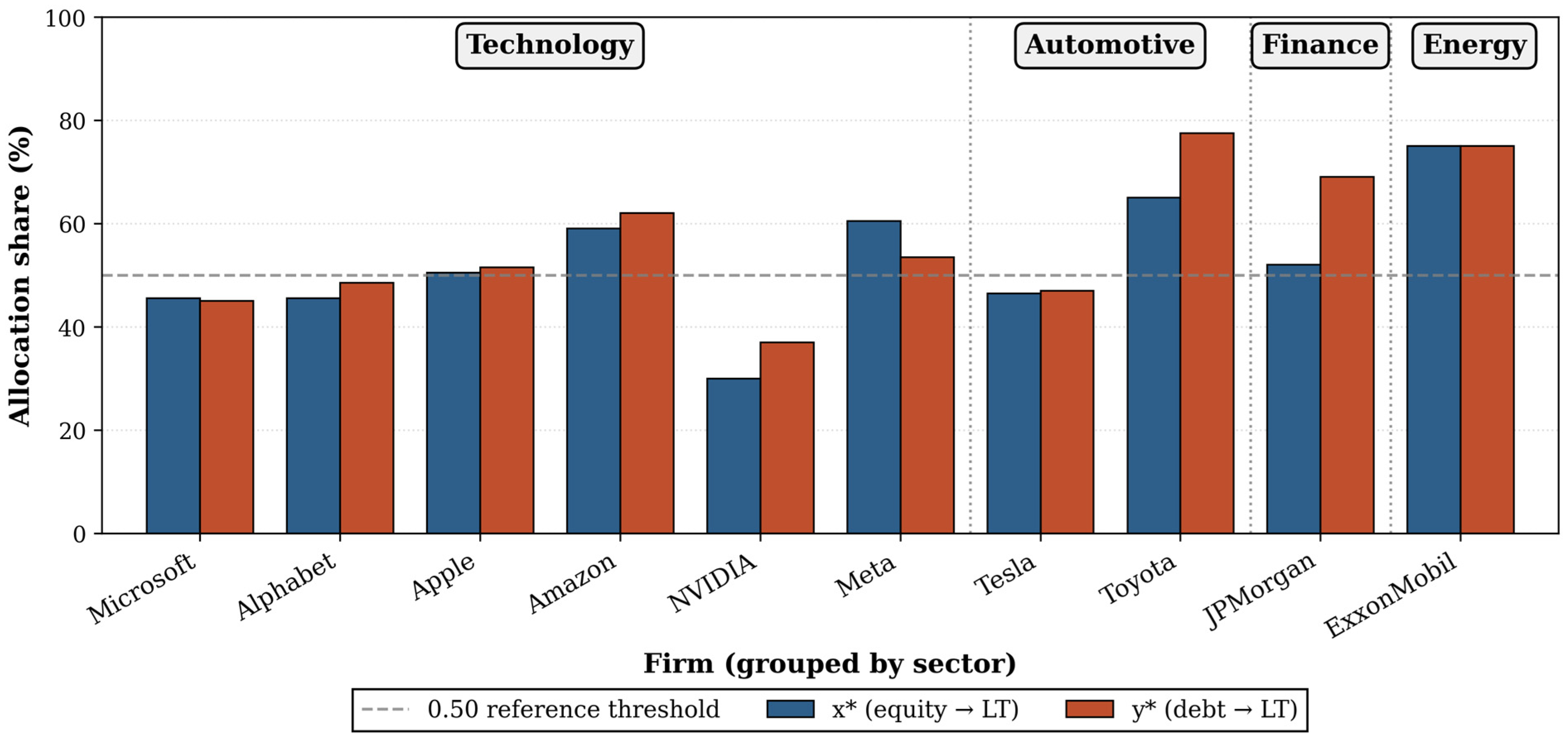
Figure 1 reveals clear sectoral stratification in ME allocation parameters. Technology firms exhibit a bimodal distribution in x* (equity-dominant versus equity-constrained), while industrial and financial firms consistently exhibit high x* values (above 50%). The y* dimension shows the most pronounced cross-firm divergence: NVIDIA (37.121%) and Microsoft (45.143%) at the low-y* pole, versus Toyota (77.477%), ExxonMobil (75.186%), JPMorgan (69.247%), and Amazon (62.094%) at the high-y* pole.

4.5. Absolute Financing Decomposition

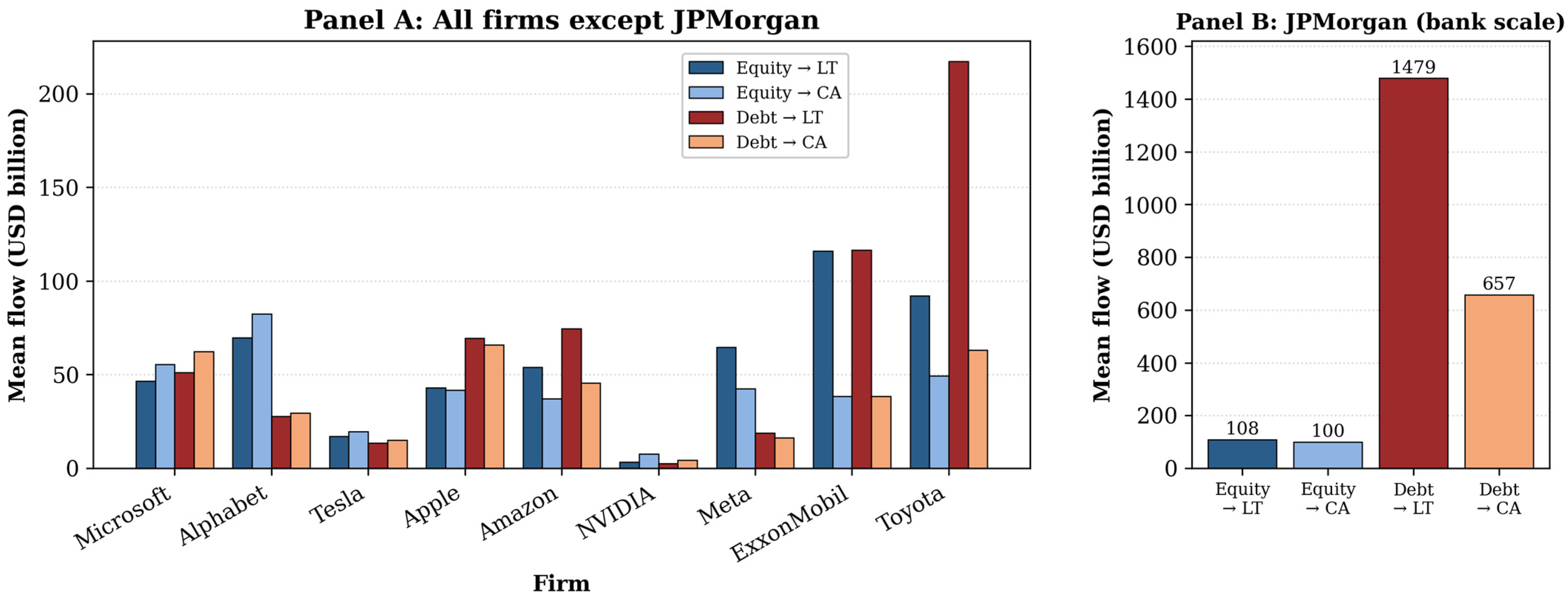
Figure 2 decomposes mean financing into four absolute flows. Microsoft allocates a mean equity-to-long-term-asset flow of approximately $46.5 B among Technology firms, with a debt-to-long-term-asset flow of approximately $51.2 B, confirming debt co-financing of Azure infrastructure. Apple’s debt-to-long-term-asset component (approximately $69.5 B) substantially exceeds its equity-to-long-term-asset component (approximately $43.0 B), so debt is the de facto long-term financing instrument in absolute dollar terms. Toyota’s decomposition is dominated by the debt-to-long-term-asset flow (approximately $217.2 B), consistent with manufacturing plant financing norms. ExxonMobil shows roughly comparable equity (approximately $116.0 B) and debt (approximately $116.5 B) contributions to long-term assets.

4.6. Shannon Entropy and Diversification Index

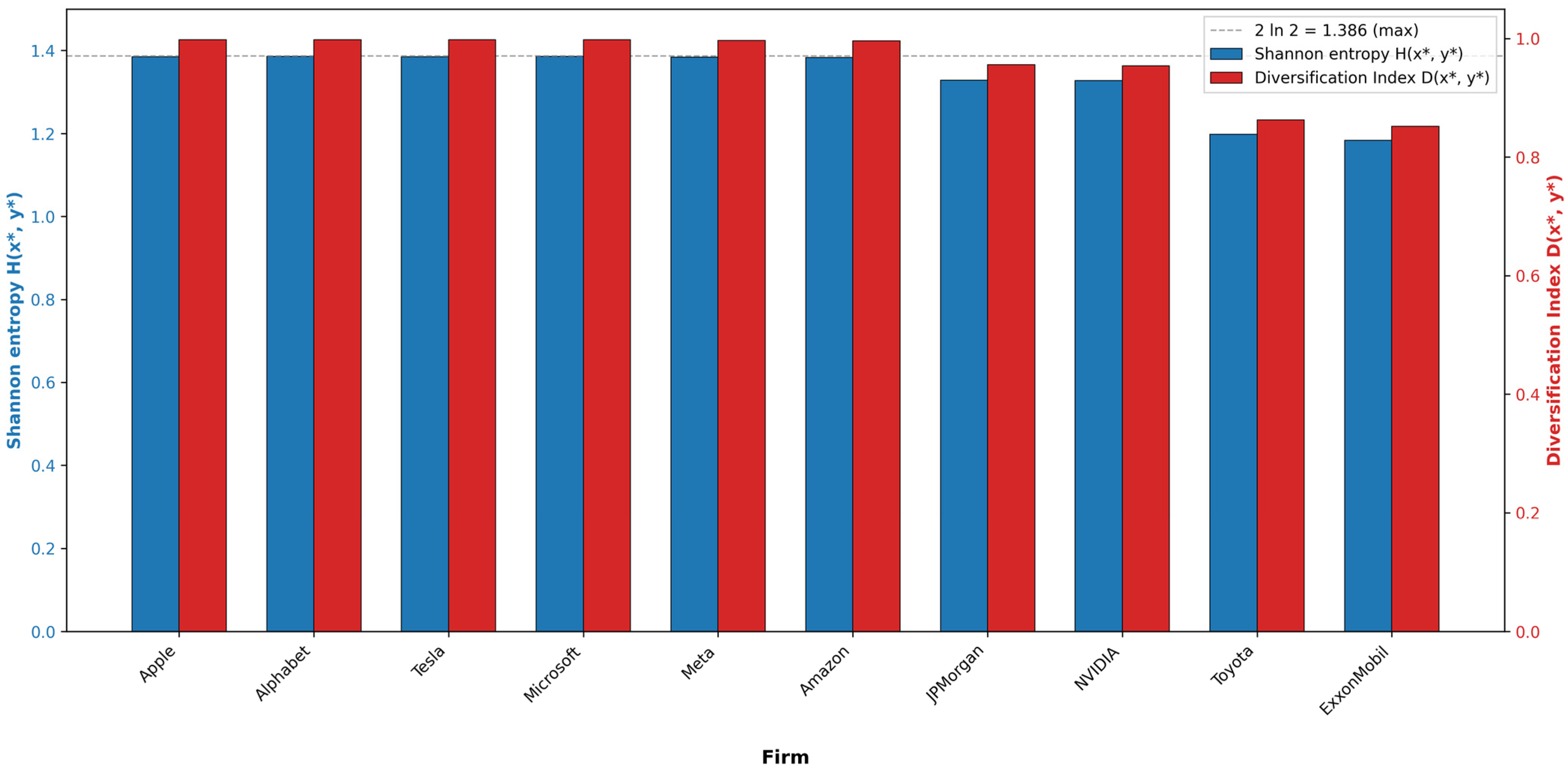
Figure 3 plots the Shannon entropy H(x*, y*) and the normalised diversification index D(x*, y*) for all ten firms, ranked by H. From Table 3, Apple records the maximum entropy in the sample (H = 1.386, D = 0.9997 at the three-decimal precision of Table 3; 0.9997 at four decimal places), a value that reflects the algebraic property that Apple’s allocation parameters (x* = 50.813%, y* = 51.300%) lie extremely close to but not exactly at the (0.5, 0.5) maximum entropy point—the corner of the (x, y) unit square at which any binary entropy is, by construction, maximised. D is below exact unity because x* ≠ y* and both differ from 0.5. We emphasise, in direct response to a referee concern about the substantive interpretation of this near-unity value, that Apple’s near-maximal D reflects this algebraic property—a feature of the balance-sheet means c ¯ and d ¯ that places almost no asymmetric tilt on the ME solution—rather than a substantive economic claim about “financing complexity” at Apple relative to other firms; a deviation of approximately 0.03% from maximum normalised entropy is not, by itself, economically informative, and we do not interpret it as such. Alphabet (H = 1.382, D = 0.997), Tesla (H = 1.382, D = 0.997), and Microsoft (H = 1.378, D = 0.994) follow closely. ExxonMobil records the lowest entropy (H = 1.121, D = 0.809), reflecting the high concentration of both equity and debt allocation toward long-term assets (x* = 75.1%, y* = 75.2%) inherent in capital-intensive extraction operations. Toyota (H = 1.180, D = 0.851) records the second-lowest entropy for similar capital-intensity reasons. Meta’s entropy (H = 1.362, D = 0.983) lies in the upper middle of the distribution; despite Meta’s strong positive alignment in M*, its (x*, y*) configuration is not particularly concentrated in either direction. Because the ME estimator explicitly maximises H subject to the balance-sheet constraint, the reported H and D values describe the entropy of the recovered solution rather than an independently observed quantity; the entropy ordering across firms therefore reflects the differential constraints the panel-mean balance sheets impose on the ME solution, not an independent empirical measurement of firm “complexity.” Two firms with the same balance sheet means c ¯ , d ¯ , and ā would receive identical entropy values by construction, whatever their underlying business behaviour. Their substantive interpretation is therefore as descriptors of allocation balance under the estimator’s information–theoretic criterion, not as direct measures of underlying randomness in firm financing behaviour. We use the term “allocation balance” rather than “complexity” throughout the manuscript wherever this distinction is relevant.

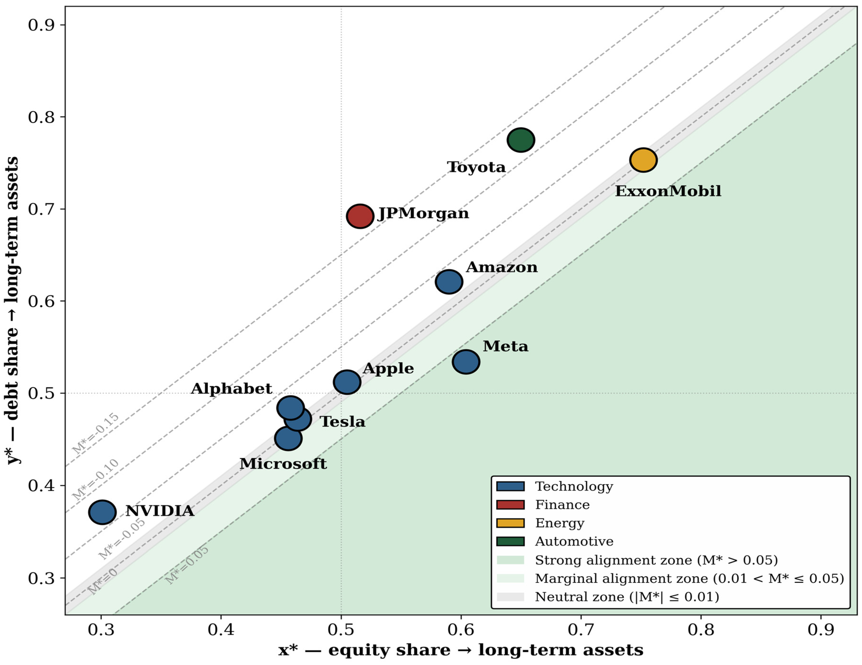
4.7. Firm Positioning in the (x*, y*) Parameter Space

Figure 4 positions all ten firms in the (x*, y*) parameter space, revealing several distinct financing archetypes consistent with the M* classification of Section 4.3: (i) the strongly aligned archetype, represented by Meta; (ii) the neutral archetype, in which M* lies within the ±1% band, represented by Microsoft, ExxonMobil, Apple (whose time-averaged x* reflects the cumulative effect of its share-repurchase programme on the panel-mean balance sheet), and Tesla; (iii) the balanced co-financing archetype, in which both x* and y* are high (Toyota, JPMorgan, Amazon); and (iv) the equity-constrained archetype (NVIDIA, and to a milder degree Alphabet, both with allocation shares below the 50% benchmark in both dimensions and x* below y*). The configuration is consistent with the conclusion of Section 4.3 that strong matching alignment is the exception rather than the rule in this sample.

4.8. Firm-Level Configurations Across Sectors

Figure 5 reports firm-level ME allocation parameters arranged by sector. We emphasise that, with only ten firms across four sectors—six in Technology, two in Automotive, and one each in Finance and Energy—any sector-level descriptive statistics computed in this sample (means, standard deviations across firms within a sector) are illustrative rather than inferentially representative of their respective sectors. We therefore present these patterns as a structured description of the present case sample, not as a generalisable statement about sectoral capital structure behaviour. The findings should be interpreted as a multi-firm case study; broader sectoral generalisations would require substantially larger and more representative samples and are left to future work.
With that caveat in mind, the following patterns are observable in the case sample. The six Technology firms exhibit considerable within-sector heterogeneity, with x* ranging from 30.1% (NVIDIA) to 60.4% (Meta) and y* ranging from 37.1% (NVIDIA) to 62.1% (Amazon). Within Automotive, Tesla and Toyota show clearly different x* values (46.4% and 65.1% respectively) and even more divergent y* values, with Toyota’s debt allocation to long-term assets well above that of Tesla in proportional terms (77.5% vs. 47.2%)—reflecting the latter’s earlier growth phase relative to Toyota’s mature manufacturing footprint. The single Finance and Energy observations (JPMorgan and ExxonMobil) each show high values of both x* and y*. We note that these single-firm sector observations echo themes in the prior literature on capital-intensive co-financing—including Adrian and Shin (2010) on banking-sector intermediation leverage, Gropp and Heider (2010) on regulatory determinants of bank capital structure, and MacKay and Phillips (2005) on industry-level capital-intensity effects—but we emphasise that one firm per sector cannot test such generalisations, and the alignment with the broader literature is offered here as descriptive context rather than as evidence that JPMorgan or ExxonMobil represents banking-sector or energy-sector financing structure more broadly. A systematic test of sector-level matching alignment across a broader cross-section of firms is an important direction for future work.

4.9. Cross-Sample Synthesis

The firm-level and sector-level analyses presented in Section 4.2, Section 4.3, Section 4.4, Section 4.5, Section 4.6, Section 4.7 and Section 4.8 admit a more general reading at the level of the entire ten-firm panel. We emphasise that the patterns reported in this section are sample-level descriptions of the present ten-firm panel and not generalisations to broader populations of firms or to specific sectors; in this sense, they are fully consistent with the case-study framing of Section 4.8. The distinction is that Section 4.8 reports patterns conditional on sector classification—where small within-sector sample sizes restrict inference—whereas the present section reports patterns observed across the panel independently of sector classification and thus avoids the small-sector-cell problem that limits Section 4.8. The patterns reported here are robust to the threshold choices examined in Section Robustness of the Classification to Alternative Thresholds. We summarise them as systematic patterns observed in the present panel, distinct from both the firm-specific case findings of Section 4.4 and Section 4.5 and the case-study sectoral patterns of Section 4.8. We use the term “patterns” deliberately to indicate descriptive sample-level observations rather than statistically validated regularities: with ten non-randomly selected firms, no confidence intervals, no regression analysis, and no hypothesis tests, the observations below cannot be claimed as empirically validated regularities in the inferential sense, and we therefore do not use that terminology.
First, strong matching alignment is rare in the sample. Of the ten firms in the panel, only one (Meta) satisfies the strong-compliance threshold M* > 0.05; no firm falls in the marginal band, and the next-closest firm (Microsoft, with M* = +0.50%) lies within the neutral band, alongside ExxonMobil, Apple, and Tesla. The remaining firms are either neutrally allocated or display moderate-to-strong negative alignment. This pattern is invariant to the threshold scheme adopted (Table 5) and is observed in firms drawn from four distinct sectors. To the extent that the present sample can be informative about the broader population of large-cap firms, the data are consistent with the view that the textbook matching prescription describes an aspirational benchmark rather than a typical empirical configuration.
Second, the dominant deviation from neutrality is in the direction of debt-financed long-term assets, not equity-financed ones. Five of the ten firms display moderate-to-strong negative alignment (M* below −0.01), while only one firm displays strong positive alignment. This asymmetry is observed across the technology, finance, energy, and automotive segments of the sample. The direction of this asymmetry is broadly consistent with the prior literature documenting structural co-financing in capital-intensive industries (MacKay & Phillips, 2005); the present sample, with one firm per non-Technology sector, cannot test such sectoral claims directly, but the pattern’s appearance across all four sectoral segments in the panel suggests that the asymmetry is not specific to capital-intensive industries and extends to the asset-light technology firms in our sample as well.
Third, the matching alignment index M* and conventional leverage capture distinct dimensions of financing structure across the firms in the present panel—but the relationship between them is more nuanced than a simple “orthogonality” claim would suggest. Pairwise correlations between conventional leverage (debt-to-equity ratio, computed from Table 2 means d ¯ / c ¯ ) and the alignment index across all ten firms yield: Pearson r(leverage, M*) = −0.750 (p = 0.012) and Pearson r(leverage, |M*|) = +0.747 (p = 0.013). The Spearman rank correlations are −0.527 (p = 0.117) and +0.200 (p = 0.580) respectively, with JPMorgan an influential outlier (leverage ≈ 10.25 reflecting banking-sector regulatory capital structure). Restricting attention to the nine non-bank firms yields r(leverage, M*) = −0.558 (p = 0.118) and r(leverage, |M*|) = +0.207 (p = 0.594). Three substantive points follow. (a) The sign of M* is moderately negatively correlated with leverage in the present sample: more highly levered firms tend to exhibit more negative M* (debt-dominant allocations), which is unsurprising given that leverage and M* both involve debt magnitudes; the association weakens and falls short of conventional significance once the banking-sector outlier is excluded, indicating that it is partly driven by JPMorgan. (b) The magnitude of misalignment, |M*|, is not statistically significantly correlated with leverage among non-bank firms, indicating that leverage does not predict how far a firm is from neutral allocation. (c) Crucially, even where a correlation exists, leverage does not characterise the firm-by-firm allocation structure: the three most strongly non-compliant firms (JPMorgan, Toyota, NVIDIA) differ markedly in their balance-sheet structure, ranging from extreme banking-sector leverage (JPMorgan), where regulatory capital structure produces an extremely low equity-to-debt ratio that approaches but does not violate the model’s interior feasibility condition (Proposition 1), to mature manufacturing leverage (Toyota, leverage ≈ 1.98), to near-minimal leverage (NVIDIA, leverage ≈ 0.62); these three firms cluster at the bottom of the M* distribution despite very different leverage profiles. Conversely, the firm with the strongest matching alignment (Meta) does have the lowest leverage in the panel, yet the next-lowest-leverage firms (Alphabet and NVIDIA) display negative alignment, indicating that low leverage alone does not guarantee matching alignment. For Apple specifically, the panel-mean leverage ratio (≈1.60) is well-defined but averages over markedly different financing regimes—a near-unlevered early-sample configuration and a repurchase-driven later configuration in which book equity declined by roughly 60% from its 2017 peak—illustrating a general limitation of ratio-based metrics that the ME framework, operating on absolute dollar values, avoids. With these qualifications, the central empirical finding is the following: leverage and M* are distinct, complementary descriptors of financing structure, and conventional leverage analysis cannot recover the firm-level allocation information that M* makes explicit; we no longer characterise this relationship as “orthogonality” in the strict statistical sense (since a moderate correlation exists for the signed index), but as a decoupling that operates at the structural–interpretation level. This decoupling demonstrates that matching alignment captures a dimension of financing structure that aggregate leverage metrics do not.
Fourth, the ME solution’s entropy H(x*, y*), interpreted as a descriptor of allocation balance under the estimator’s information–theoretic criterion (Section 4.6), orders firms in a way that is not recovered by firm size, leverage, or sector classification in the present sample. The maximum entropy firm (Apple) and the minimum entropy firm (ExxonMobil) are of broadly comparable balance-sheet magnitude, while Alphabet and Tesla achieve essentially identical entropy values (H = 1.382) despite differing by roughly a factor of four in balance-sheet size; each firm achieves its entropy rank because its balance-sheet means ( c ¯ , d ¯ , ā) place the ME solution near the centre of the unit square (Apple, Alphabet, Tesla) or near the high-allocation corner (ExxonMobil), rather than because of its scale or leverage. We emphasise that this is a property of the ME solution under the imposed balance-sheet constraints, not an independent empirical discovery about “complexity” in firm financing behaviour; the cross-firm entropy ordering is reproducible by anyone applying the same estimator to the same balance-sheet means. With this qualification, the pattern observed in the present sample is consistent with the broader claim—articulated in the Introduction—that observable financing ratios are insufficient statistics for the underlying financing allocation structure: two firms with very different conventional ratios can yield similar ME-solution entropies, and vice versa.
These four cross-sample observations are stated as descriptive patterns observed in the present ten-firm panel. They are descriptive rather than statistically validated: the sample size is small and non-random, and we do not report confidence intervals, regression estimates, or hypothesis tests for these patterns. They do not require the panel to be statistically representative of any specific sector, country, or firm-size class, and they are therefore not subject to the small-sample sectoral-inference concerns appropriately raised in Section 4.8. Their generalisability to broader populations of firms is an empirical question that must be settled with larger and more representative samples; we discuss this and other directions for future work in the concluding section.

5. Conclusions

This paper has developed and applied a maximum entropy panel estimator to resolve a fundamental identification problem in empirical capital structure research: the unobservability of internal financing allocation across asset categories from standard balance-sheet data. By maximising joint Shannon entropy subject to a mean-level balance-sheet constraint, the estimator recovers two latent scalar parameters—the equity allocation share x* and the debt allocation share y* directed toward long-term asset financing—without imposing parametric assumptions beyond the balance-sheet identity. The Lagrange multiplier λ* provides a cardinal financing pressure index interpretable through the envelope theorem, and the continuous matching alignment index M* = x* − y* provides a finely graded measure of structural compliance with the financial matching principle, free from the internal sign inconsistency that affects binary x* > 0.5 ∧ y* < 0.5 criteria within the single-multiplier ME framework. Bisection convergence is guaranteed within 21 iterations, rendering the framework suitable for large-scale panel applications.
Applied to a ten-firm, cross-sectoral panel spanning up to 25 years (with firm-specific subperiods), the framework yields findings at three distinct levels of generality, which we report separately to avoid conflating them.
At the methodological level, the contributions are sample-independent and apply to any balance-sheet panel satisfying the basic feasibility condition of Proposition 1. The maximum entropy estimator, the closed-form logistic representation, the bisection algorithm with its 21-iteration convergence bound, the financing pressure index λ*, the continuous matching alignment index M*, and the robustness framework of Section Robustness of the Classification to Alternative Thresholds are general-purpose tools that do not depend on the particular ten firms used here for illustration.
At the cross-sample empirical level (Section 4.9), four patterns are observed across the present ten-firm panel independently of sector. First, strong matching alignment is rare in the sample: only Meta achieves M* > 0.05, while five firms display moderate-to-strong negative alignment. Second, the dominant deviation from neutrality is toward debt-financed long-term assets, not equity-financed ones—a pattern observed across all four sectors represented in the panel. Third, M* and conventional leverage capture distinct dimensions of financing structure: although the signed index is moderately correlated with leverage in the sample (Pearson r = −0.75, p = 0.012 across all ten firms), the magnitude of misalignment |M*| is not statistically significantly correlated with leverage among non-bank firms (r = +0.21, p = 0.59), and the firm-by-firm allocation structure that M* reveals—including firms with very different leverage profiles clustering at the same end of the M* distribution, and low leverage alone not guaranteeing matching alignment—cannot be recovered from leverage analysis alone; Apple, whose ratio-based leverage averages over markedly different financing regimes following the steep repurchase-driven erosion of its book equity, is handled naturally by the ME framework, which operates on absolute dollar values rather than ratios. Fourth, Shannon entropy of the (x*, y*) configuration similarly captures structural information that firm size, leverage, and sector classification do not recover. These four patterns are descriptive sample-level observations about the present panel rather than statistically validated regularities; their generalisability to broader populations is an empirical question for future work.
At the case-specific level, the framework reveals firm-level configurations that aggregate leverage analysis cannot characterise. Apple’s sustained share-repurchase programme has steeply eroded its book equity, which declined by roughly 60% from its 2017 peak while remaining positive; although Apple’s proportional allocation shares fall within the neutral band at the panel-mean level (M* = −0.49%), in absolute dollar terms its debt-to-long-term-asset flow (approximately $69.5 B) substantially exceeds its equity flow (approximately $43.0 B), so that debt remains the dominant long-term financing instrument in dollar terms—a finding with direct implications for financial risk assessment. NVIDIA’s fabless business model translates into the lowest x* in the panel (30.1%), consistent with its minimal long-term physical asset base. JPMorgan’s banking-intermediation structure produces persistently high y* and persistently low equity-to-debt ratios and yields the most pronounced negative matching alignment in the sample (M* = −17.3%). These case-specific findings are illustrative of the kinds of structural configurations the framework can identify and should be interpreted as case-study evidence rather than as generalisations.
These findings carry implications for theory, practice, and regulation. For theory, the results challenge leverage-centric representations of capital structure by demonstrating that identical leverage ratios are consistent with structurally distinct financing configurations. For practice, λ* and M* together provide risk analysts with two complementary, balance-sheet-consistent measures of financing structure—one of concentration, one of matching alignment—that complement conventional metrics. For regulators, the decomposition of financing flows offers a more granular diagnostic of systemic vulnerability than aggregate debt ratios.
Several limitations define directions for future research. First, the time-invariance assumption on (x, y) precludes identification of structural breaks; rolling-window or regime-switching ME estimation could address this and would also speak directly to the question of whether financing entropy and M* behave procyclically or countercyclically. Second, the sample is restricted to ten large-cap U.S. and Japanese firms; the present results should accordingly be read as a multi-firm case study, and a systematic test of cross-sectoral matching alignment requires substantially broader and more representative samples covering additional firms in each sector, additional sectors, additional countries, and small-cap and mid-cap firms. Third, incorporating additional moment conditions—interest coverage ratios, debt maturity schedules where available—could sharpen identification further. Fourth, whether M* serves as a leading indicator of financial distress is an empirical question that the present statistical analysis cannot answer; out-of-sample testing on a panel including distressed firms is a natural next step.

Supplementary Materials

The following supporting information can be downloaded at: https://www.mdpi.com/article/10.3390/jrfm19060439/s1. S1: Data Description; S2: Estimation Algorithm; S3: Additional Tables; S4: Code Availability.

Funding

This research received no external funding.

Institutional Review Board Statement

Not applicable.

Informed Consent Statement

Not applicable.

Data Availability Statement

The data used in this study are publicly available from Macrotrends (https://www.macrotrends.net). The datasets analyzed during the current study were obtained from publicly accessible company financial statements and market data-bases available through Macrotrends. The processed data supporting the findings of this study are available from the corresponding author upon reasonable request.

Acknowledgments

During the preparation of this work, the author used Claude Sonnet 4.6 (Anthropic, 2024) in order to improve the language, clarity, and readability of the manuscript. After using this tool, the author reviewed and edited the content as needed and takes full responsibility for the content of the published article.

Conflicts of Interest

The authors declare no conflict of interest.

References

  1. Acharya, V. V., Almeida, H., & Campello, M. (2007). Is cash negative debt? A hedging perspective on corporate financial policies. Journal of Financial Intermediation, 16(4), 515–554. [Google Scholar] [CrossRef]
  2. Adrian, T., & Shin, H. S. (2010). Liquidity and leverage. Journal of Financial Intermediation, 19(3), 418–437. [Google Scholar] [CrossRef]
  3. Almeida, H., & Campello, M. (2007). Financial constraints, asset tangibility, and corporate investment. Review of Financial Studies, 20(5), 1429–1460. [Google Scholar] [CrossRef]
  4. Anthropic. (2024). Claude (large language model). Anthropic, PBC. Available online: https://www.anthropic.com (accessed on 25 March 2026).
  5. Avellaneda, M., Friedman, C., Holmes, R., & Samperi, D. (1997). Calibrating volatility surfaces via relative-entropy minimization. Applied Mathematical Finance, 4(1), 37–64. [Google Scholar] [CrossRef]
  6. Bacchetta, M., Beverelli, C., Cadot, O., Fugazza, M., Grether, J.-M., Helble, M., Nicita, A., & Piermartini, R. (2012). A practical guide to trade policy analysis. World Trade Organization; UNCTAD. [Google Scholar]
  7. Baker, M., & Wurgler, J. (2002). Market timing and capital structure. Journal of Finance, 57(1), 1–32. [Google Scholar] [CrossRef]
  8. Barclay, M. J., & Smith, C. W. (1995). The maturity structure of corporate debt. Journal of Finance, 50(2), 609–631. [Google Scholar] [CrossRef]
  9. Billett, M. T., King, T. H. D., & Mauer, D. C. (2007). Growth opportunities and the choice of leverage, debt maturity, and covenants. Journal of Finance, 62(2), 697–730. [Google Scholar] [CrossRef]
  10. Bowden, R. J. (2011). Directional entropy and tail uncertainty, with applications to financial hazard. Quantitative Finance, 11(3), 437–446. [Google Scholar] [CrossRef]
  11. Bradley, M., Jarrell, G. A., & Kim, E. H. (1984). On the existence of an optimal capital structure: Theory and evidence. Journal of Finance, 39(3), 857–878. [Google Scholar] [CrossRef]
  12. Brav, A., Graham, J. R., Harvey, C. R., & Michaely, R. (2005). Payout policy in the 21st century. Journal of Financial Economics, 77(3), 483–527. [Google Scholar] [CrossRef]
  13. Buchen, P. W., & Kelly, M. (1996). The maximum entropy distribution of an asset inferred from option prices. Journal of Financial and Quantitative Analysis, 31(1), 143–159. [Google Scholar] [CrossRef]
  14. Cabrales, A., Gottardi, P., & Vega-Redondo, F. (2017). Risk sharing and contagion in networks. Review of Financial Studies, 30(9), 3086–3127. [Google Scholar] [CrossRef]
  15. Campello, M., Lin, C., Ma, Y., & Zou, H. (2011). The real and financial implications of corporate hedging. Journal of Finance, 66(5), 1615–1647. [Google Scholar] [CrossRef]
  16. Chernenko, S., & Faulkender, M. (2012). The two sides of derivatives usage: Hedging and speculating with interest rate swaps. Journal of Financial and Quantitative Analysis, 47(6), 1727–1754. [Google Scholar] [CrossRef]
  17. DeMiguel, V., Garlappi, L., & Uppal, R. (2009). Optimal versus naive diversification: How inefficient is the 1/N portfolio strategy? Review of Financial Studies, 22(5), 1915–1953. [Google Scholar] [CrossRef]
  18. Fama, E. F., & French, K. R. (2001). Disappearing dividends: Changing firm characteristics or lower propensity to pay? Journal of Financial Economics, 60(1), 3–43. [Google Scholar] [CrossRef]
  19. Fama, E. F., & French, K. R. (2005). Financing decisions: Who issues stock? Journal of Financial Economics, 76(3), 549–582. [Google Scholar] [CrossRef]
  20. Faulkender, M. (2005). Hedging or market timing? Selecting the interest rate exposure of corporate debt. Journal of Finance, 60(2), 931–962. [Google Scholar] [CrossRef]
  21. Faulkender, M., Flannery, M. J., Hankins, K. W., & Smith, J. M. (2012). Cash flows and leverage adjustments. Journal of Financial Economics, 103(3), 632–646. [Google Scholar] [CrossRef]
  22. Fischer, E. O., Heinkel, R., & Zechner, J. (1989). Dynamic capital structure choice: Theory and tests. Journal of Finance, 44(1), 19–40. [Google Scholar] [CrossRef]
  23. Frank, M. Z., & Goyal, V. K. (2003). Testing the pecking order theory of capital structure. Journal of Financial Economics, 67(2), 217–248. [Google Scholar] [CrossRef]
  24. Frank, M. Z., & Goyal, V. K. (2009). Capital structure decisions: Which factors are reliably important? Financial Management, 38(1), 1–37. [Google Scholar] [CrossRef]
  25. Golan, A., Judge, G., & Miller, D. (1996). Maximum entropy econometrics: Robust estimation with limited data. John Wiley & Sons. [Google Scholar]
  26. Goldstein, R., Ju, N., & Leland, H. (2001). An EBIT-based model of dynamic capital structure. Journal of Business, 74(4), 483–512. [Google Scholar] [CrossRef] [PubMed]
  27. Graham, J. R., & Leary, M. T. (2011). A review of empirical capital structure research and directions for the future. Annual Review of Financial Economics, 3(1), 309–345. [Google Scholar] [CrossRef]
  28. Graham, J. R., Lemmon, M. L., & Wolf, J. G. (2002). Does corporate diversification destroy value? Journal of Finance, 57(2), 695–720. [Google Scholar] [CrossRef]
  29. Gropp, R., & Heider, F. (2010). The determinants of bank capital structure. Review of Finance, 14(4), 587–622. [Google Scholar] [CrossRef]
  30. Guedes, J., & Opler, T. (1996). The determinants of the maturity of corporate debt issues. Journal of Finance, 51(5), 1809–1833. [Google Scholar] [CrossRef]
  31. Harris, M., & Raviv, A. (1991). The theory of capital structure. Journal of Finance, 46(1), 297–355. [Google Scholar] [CrossRef]
  32. Hart, O., & Moore, J. (1994). A theory of debt based on the inalienability of human capital. Quarterly Journal of Economics, 109(4), 841–879. [Google Scholar] [CrossRef]
  33. Jaynes, E. T. (1957). Information theory and statistical mechanics. Physical Review, 106(4), 620–630. [Google Scholar] [CrossRef]
  34. Kahle, K. M., & Stulz, R. M. (2017). Is the US public corporation in trouble? Journal of Economic Perspectives, 31(3), 67–88. [Google Scholar] [CrossRef]
  35. Kraus, A., & Litzenberger, R. H. (1973). A state-preference model of optimal financial leverage. Journal of Finance, 28(4), 911–922. [Google Scholar] [CrossRef]
  36. Lazonick, W. (2014). Profits without prosperity. Harvard Business Review, 92(9), 46–55. [Google Scholar]
  37. Lemmon, M. L., Roberts, M. R., & Zender, J. F. (2008). Back to the beginning: Persistence and the cross-section of corporate capital structure. Journal of Finance, 63(4), 1575–1608. [Google Scholar] [CrossRef]
  38. MacKay, P., & Phillips, G. M. (2005). How does industry affect firm financial structure? Review of Financial Studies, 18(4), 1433–1466. [Google Scholar] [CrossRef]
  39. Mercurio, P. J., Wu, Y., & Xie, H. (2020). An entropy-based approach to portfolio optimization. Entropy, 22(3), 332. [Google Scholar] [CrossRef] [PubMed]
  40. Modigliani, F., & Miller, M. H. (1958). The cost of capital, corporation finance and the theory of investment. American Economic Review, 48(3), 261–297. [Google Scholar]
  41. Modigliani, F., & Miller, M. H. (1963). Corporate income taxes and the cost of capital: A correction. American Economic Review, 53(3), 433–443. [Google Scholar]
  42. Morris, J. R. (1976). On corporate debt maturity strategies. Journal of Finance, 31(1), 29–37. [Google Scholar] [CrossRef]
  43. Myers, S. C. (1977). Determinants of corporate borrowing. Journal of Financial Economics, 5(2), 147–175. [Google Scholar] [CrossRef]
  44. Myers, S. C. (1984). The capital structure puzzle. Journal of Finance, 39(3), 574–592. [Google Scholar] [CrossRef]
  45. Myers, S. C., & Majluf, N. S. (1984). Corporate financing and investment decisions when firms have information that investors do not have. Journal of Financial Economics, 13(2), 187–221. [Google Scholar] [CrossRef]
  46. Philippatos, G. C., & Wilson, C. J. (1972). Entropy, market risk, and the selection of efficient portfolios. Applied Economics, 4(3), 209–220. [Google Scholar] [CrossRef]
  47. Rajan, R. G., & Zingales, L. (1995). What do we know about capital structure? Some evidence from international data. Journal of Finance, 50(5), 1421–1460. [Google Scholar] [CrossRef]
  48. Rauh, J. D., & Sufi, A. (2010). Capital structure and debt structure. Review of Financial Studies, 23(12), 4242–4280. [Google Scholar] [CrossRef]
  49. Scott, J. H. (1976). A theory of optimal capital structure. Bell Journal of Economics, 7(1), 33–54. [Google Scholar] [CrossRef] [PubMed]
  50. Shannon, C. E. (1948). A mathematical theory of communication. Bell System Technical Journal, 27(3), 379–423. [Google Scholar] [CrossRef]
  51. Shyam-Sunder, L., & Myers, S. C. (1999). Testing static trade-off against pecking order models of capital structure. Journal of Financial Economics, 51(2), 219–244. [Google Scholar] [CrossRef]
  52. Stohs, M. H., & Mauer, D. C. (1996). The determinants of corporate debt maturity structure. Journal of Business, 69(3), 279–312. [Google Scholar] [CrossRef] [PubMed]
  53. Stutzer, M. (1996). A simple nonparametric approach to derivative security valuation. Journal of Finance, 51(5), 1633–1652. [Google Scholar] [CrossRef]
  54. Titman, S., & Wessels, R. (1988). The determinants of capital structure choice. Journal of Finance, 43(1), 1–19. [Google Scholar] [CrossRef]
  55. Usta, I., & Kantar, Y. M. (2011). Mean-variance-skewness-entropy measures: A multi-objective approach for portfolio selection. Entropy, 13(1), 117–133. [Google Scholar] [CrossRef]
  56. Welch, I. (2004). Capital structure and stock returns. Journal of Political Economy, 112(1), 106–131. [Google Scholar] [CrossRef]
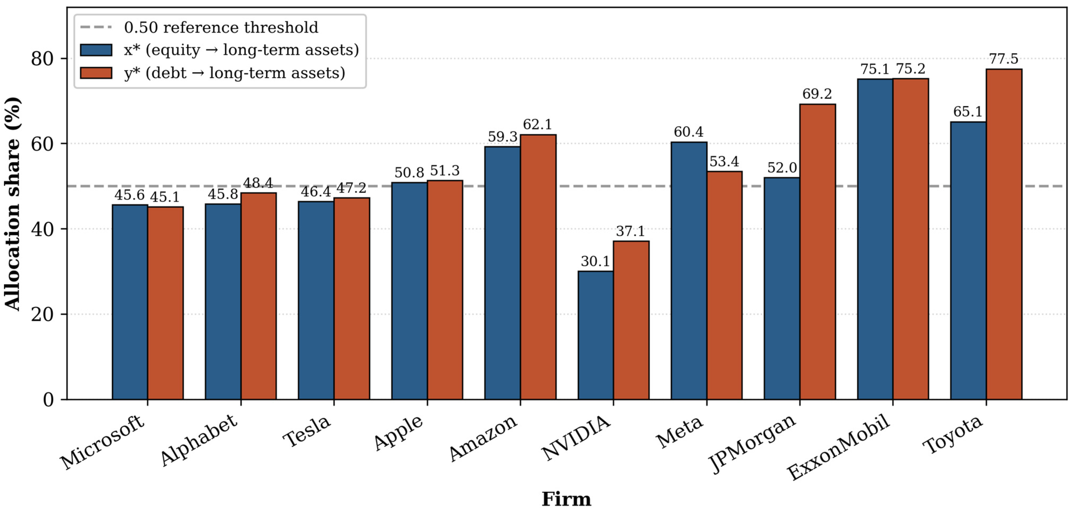
Figure 1. ME estimates of financing allocation parameters x* (equity → long-term assets) and y* (debt → long-term assets) for the ten-firm panel. Dashed line = 0.50 reference threshold. All values were computed via the bisection algorithm with ε = 10−5.
Jrfm 19 00439 g001
Figure 2. Absolute financing structure decomposition into four mean flows: equity → LT (x* · c ¯ ), equity → CA ((1 − x*) · c ¯ ), debt → LT (y* · d ¯ ), debt → CA ((1 − y*) · d ¯ ). For visual comparability across the very different balance-sheet scales of the panel firms, all firms’ values are reported on a common scale; JPMorgan’s series, given its bank scale, is shown on a separate panel to preserve resolution. LT = long-term assets; CA = current assets.
Jrfm 19 00439 g002
Figure 3. Shannon entropy H(x*, y*) (left axis) and normalised diversification index D(x*, y*) = H/(2 ln 2) (right axis) for all ten firms, ranked by H. Maximum entropy 2 ln 2 ≈ 1.386 corresponds to D = 1.0 (perfectly balanced allocation).
Jrfm 19 00439 g003
Figure 4. Firm positioning in the (x*, y*) parameter space. Each point represents one firm’s ME allocation estimates. Iso-M* contour lines (M* = +0.05, 0, −0.05, −0.10, −0.15) are shown to facilitate interpretation. Shaded regions follow the classification scheme of Section 3.6: darker green = strong alignment zone (M* > 0.05); lighter green = marginal alignment zone (0.01 < M* ≤ 0.05); pale grey = neutral zone (|M*| ≤ 0.01). The marginal alignment band is shown for completeness as part of the a priori classification scheme defined in Table 1, although no firm in the present ten-firm sample falls within it (the empty band is itself an empirical finding of the analysis, reported in Section 4.3); shading the band reflects the classification scheme rather than the sample distribution. The shaded zones are descriptive labels overlaid on the continuous (x*, y*) plane; the analytically relevant object is the continuous index M*, whose firm-level values are reported in Table 3 and Table 4 and whose ranking is invariant to threshold choice. Annotations show firm names; colours indicate sectors.
Jrfm 19 00439 g004
Figure 5. Firm-level ME allocation parameters arranged by sector. Dark bars = x*; light bars = y*. Dashed line = 0.50 reference threshold. Sector labels are descriptive of the firms in the case sample, not inferentially representative of the broader sectors.
Jrfm 19 00439 g005
Table 1. Matching alignment classification scheme.
CategoryCriterionInterpretation
Strong compliantM* > 0.05Equity is the dominant long-term financing source by a margin of more than 5 percentage points.
Marginal compliant0.01 < M* ≤ 0.05Equity allocation slightly exceeds debt allocation; alignment is positive but modest.
Neutral−0.01 ≤ M* ≤ 0.01Equity and debt are allocated to long-term assets in essentially equal proportions; no meaningful alignment in either direction.
Moderate non-compliant−0.10 < M* < −0.01Debt allocation moderately exceeds equity allocation; structural departure from the matching benchmark.
Strong non-compliantM* ≤ −0.10Debt is the dominant long-term financing source by a margin of ten percentage points or more.
Note: M* = x* − y* is the matching alignment index defined in Equation (26). Thresholds are chosen to yield economically interpretable categories spanning the empirical range observed in the present sample.
Table 2. Descriptive statistics of balance-sheet variables (USD billion).
Firm (Ticker)SectorPeriodnāSD(a) b ¯ SD(b) c ¯ SD(c) d ¯ SD(d)
Microsoft (MSFT)Technology2001–20252597.755.881.677.4101.883.2113.579.6
Alphabet (GOOGL)Technology2004–20252297.265.1109.5108.4152.0115.257.055.1
Tesla (TSLA)Automotive2014–20251230.424.338.024.336.730.228.318.5
Apple (AAPL)Technology2001–202525112.578.289.064.884.746.3135.499.8
Amazon (AMZN)Technology2004–202421128.5111.861.457.991.189.3120.0108.2
NVIDIA (NVDA)Technology2001–2025255.88.211.018.410.920.46.88.8
Meta (META)Technology2012–20241383.454.851.131.9107.272.135.028.3
JPMorgan (JPM)Finance2001–2024241587586680268208.491.62136742
ExxonMobil (XOM)Energy2001–202424232.551.866.019.9154.451.2155.039.4
Toyota (TM)Automotive2001–202424309.2119.4100.834.1141.367.5280.4103.8
Note: a = long-term assets; b = current assets; c = equity capital; d = total liabilities. ā, b ¯ , c ¯ , d ¯ = sample means; SD = standard deviation. JPMorgan values in USD billion at full bank scale.
Table 3. Maximum entropy estimates of financing allocation parameters for the ten-firm panel.
FirmSectorx* (%)y* (%)1 − x* (%)1 − y* (%)λ*H(x*, y*)D(x*, y*)|error|
MicrosoftTechnology45.64145.14354.35954.8570.00171.3780.994<10−3
AlphabetTechnology45.79248.41954.20851.5810.00111.3820.997<10−3
TeslaAutomotive46.41247.23253.58852.7680.00391.3820.997<10−3
AppleTechnology50.81351.30049.18748.700−0.00041.3860.9997<10−3
AmazonTechnology59.25962.09440.74137.906−0.00411.3400.966<10−3
NVIDIATechnology30.05337.12169.94762.8790.07751.2710.917<10−3
MetaTechnology60.35653.42639.64446.574−0.00391.3620.983<10−3
JPMorganFinance51.97969.24748.02130.753−0.00041.3090.945<10−3
ExxonMobilEnergy75.10675.18624.89424.814−0.00721.1210.809<10−3
ToyotaAutomotive65.08077.47734.9222.523−0.00441.1800.851<10−3
Note: x* = equity share → long-term assets; y* = liabilities share → long-term assets; λ* = Lagrange multiplier; H = Shannon entropy; D = H/(2 ln 2); |error| = relative constraint-satisfaction error | c ¯ x* + d ¯ y* − ā|/ā.
Table 4. Matching alignment index and financing-strategy classification.
FirmSectorx* (%)y* (%)M* (%)Classificationλ* SignFinancing Strategy
MetaTechnology60.35653.426+6.931Strong compliantNeg (−)Equity-led long-term financing backed by strong internal cash generation
MicrosoftTechnology45.64145.143+0.498NeutralPos (+)Near-even split of both sources; debt co-finances cloud infrastructure
ExxonMobilEnergy75.10675.186−0.0802NeutralNeg (−)Symmetric equity–debt co-financing of capital-intensive long-term assets
AppleTechnology50.81351.300−0.486NeutralNeg (−)Buyback-driven equity depletion; debt dominant in absolute dollar terms
TeslaAutomotive46.41247.232−0.819NeutralPos (+)Growth-phase allocation with both shares just below the 50% benchmark
AlphabetTechnology45.79248.419−2.627Moderate non-compliantPos (+)Cash-rich, current-asset-tilted; mildly debt-led long-term financing
AmazonTechnology59.25962.094−2.835Moderate non-compliantNeg (−)Debt-financed cloud-infrastructure buildout
NVIDIATechnology30.05337.121−7.068Moderate non-compliantPos (+)Equity-constrained, asset-light fabless model
ToyotaAutomotive65.08077.477−12.397Strong non-compliantNeg (−)Conventional manufacturing debt co-financing of plant and equipment
JPMorganFinance51.97969.247−17.268Strong non-compliantNeg (−)Banking intermediation: long-term credit assets predominantly debt-funded
Note: M* ≡ x* − y* is the matching alignment index (Equation (26)). Classification follows Table 1. Firms are ordered by M* from most strongly compliant to most strongly non-compliant. LT = long-term assets.
Table 5. Robustness of the matching alignment classification to alternative threshold sets.
FirmM* (%)Baseline: ±0.01, ±0.05, ±0.10Narrower: ±0.005, ±0.03, ±0.08Wider: ±0.02, ±0.07, ±0.15Quartile-Based: ±0.005, ±0.027, ±0.070
Meta+6.931Strong compliantStrong compliantMarginal compliantStrong compliant
Microsoft+0.498NeutralNeutralNeutralNeutral
ExxonMobil−0.0802NeutralNeutralNeutralNeutral
Apple−0.486NeutralNeutralNeutralNeutral
Tesla−0.819NeutralModerate non-compliantNeutralModerate non-compliant
Alphabet−2.627Moderate non-compliantModerate non-compliantModerate non-compliantModerate non-compliant
Amazon−2.835Moderate non-compliantModerate non-compliantModerate non-compliantModerate non-compliant
NVIDIA−7.068Moderate non-compliantModerate non-compliantModerate non-compliantStrong non-compliant
Toyota−12.397Strong non-compliantStrong non-compliantModerate non-compliantStrong non-compliant
JPMorgan−17.268Strong non-compliantStrong non-compliantStrong non-compliantStrong non-compliant
Note: M* ≡ x* − y* is the matching alignment index (Equation (26)). Each column applies the indicated threshold set to all ten firms. Firms are ordered by M* from most strongly compliant to most strongly non-compliant. Threshold sets are: Baseline = the classification adopted in Table 1; narrower = a tighter scheme; wider = a more permissive scheme; quartile-based = thresholds equal to the first quartile, median, and third quartile of the empirical |M*| distribution.
Disclaimer/Publisher’s Note: The statements, opinions and data contained in all publications are solely those of the individual author(s) and contributor(s) and not of MDPI and/or the editor(s). MDPI and/or the editor(s) disclaim responsibility for any injury to people or property resulting from any ideas, methods, instructions or products referred to in the content.