

The Black Hole Universe, Part I


1
Institute of Space Sciences (ICE, CSIC), 08193 Barcelona, Spain
2
Institut d Estudis Espacials de Catalunya (IEEC), 08034 Barcelona, Spain
Symmetry 2022, 14(9), 1849; https://doi.org/10.3390/sym14091849
Submission received: 12 August 2022
/
Revised: 31 August 2022
/
Accepted: 2 September 2022
/
Published: 5 September 2022
(This article belongs to the Special Issue Nature and Origin of Dark Matter and Dark Energy)
Abstract
:The original Friedmann (1922) and Lemaitre (1927) cosmological model corresponds to a classical solution of General Relativity (GR), with the same uniform (FLRW) metric as the standard cosmology, but bounded to a sphere of radius R and empty space outside. We study the junction conditions for R to show that a co-moving observer, like us, located anywhere inside R, measures the same background and has the same past light-cone as an observer in an infinite FLRW with the same density. We also estimate the mass M inside R and show that in the observed universe GM, which corresponds to a Black Hole Universe (BHU). We argue that this original Friedmann–Lemaitre model can explain the observed cosmic acceleration without the need of Dark Energy, because acts like a cosmological constant . The same solution can describe the interior of a stellar or galactic BHs. In co-moving coordinates the BHU is expanding while in physical or proper coordinates it is asymptotically static. Such frame duality corresponds to a simple Lorentz transformation. The BHU therefore provides a physical BH solution with an asymptotically deSitter metric interior that merges into a Schwarzschild metric exterior without discontinuities.
1. Introduction
A Schwarzschild black hole (BH) metric (SBH, in Equation (A12)) corresponds to a singular object of mass M, whose event horizon, GM, prevents getting information from the interior to any exterior observer. Physically, a singular point does not make much sense. The concept of physical infinity is not a scientific one if science involves testability by either observation or experiment [1]. So if the SBH is not a proper physical solution all the way to , are there other physical solutions for the metric inside observed BHs? The internal metric and BH content are in fact important to understand gravitational wave emission, BH interactions, BH formation or the origin of BHs as dark matter candidates (see Refs. [2,3] and references for some discussion). We look here for an alternative solution to the SBH interior, defined as an object of energy-mass M and size that reproduces the SBH metric, i.e., it is approximately empty, on the outside . The corresponding mean energy density at GM, as measured by an observer outside (in flat empty space) is:
regardless of its contents. Even when the BH is static outside, a static solution for the BH interior cannot exist for regular matter or radiation because it requires a minimal Buchdahl radius [4]: , which is larger than and it is therefore not a BH (the mass inside is smaller than , so there is no event horizon). However, objects with external mass M and sizes have been observed. What is then inside a BH? For a perfect fluid, to achieve such a density, the radial pressure inside a BH needs to be negative (see Ref. [5] and references therein). Cosmologist are used to this type of fluids, which are called Quintessence, Inflation, or Dark Energy (DE). Could the inside of a BH be DE [6]? Could it also be an expanding universe, like ours? If so, what can this tell us about our universe?
Here, we explore this idea more generally: a non static but uniform GR solution inside a finite R that we call the FLRW cloud (or FLRW*) based on the Lemaitre [7] cosmological model. As it is well known (see, e.g., Ref. [8]), it was Lemaitre who first published and realised the meaning and implications of the distance-redshift relation () that made Hubble famous. Lemaitre noticed that this was a consequence of Einstein’s new theory of gravity described by the (later known as) Friedmann–Lemaitre–Robertson–Walker (FLRW) flat metric in co-moving coordinates , which corresponds to an homogeneous and isotropic (usually assumed infinite) space-time:
For a perfect fluid with density and pressure p, the solution to GR field equations is well-known. The different energy conservation and acceleration equations reduced to (see Equation (10).73 in Ref. [9]):
where and , where and represents the current () matter and radiation density, respectively, and . The cosmological constant term results from: . This is the standard cosmological (CDM ) model. Given , we can solve Equation (3) to find . In this paper, we will use these same equations to make the two points below, which will be discussed in more detail in the corresponding section as shown:
- Section 2: A FLRW cloud (FLRW*) is also a GR solution. The FLRW metric with a finite spherical volume of proper radius is also a GR solution. When FLRW* is inside its Schwarzschild radius and the space outside can be approximated as empty, this is a BHU. This solution for a BH interior is different from the SBH solution.
- Section 3: A BHU without DE has the same observable background as ΛCDM. The observed cosmic acceleration can be understood as resulting from a BHU without DE, where GM acts like as an effective term, with . A co-moving observer, anywhere within R in a BHU, sees the same background as an observer in the CDM with the same density.
Section 2 and Section 3 are dedicated to each of the points above. As we will show, the existence of the FLRW* solution is not a new result but its interpretation in the light of the observed cosmic acceleration and the BHU is new. In Section 2.2 we present a new calculation of junction conditions for the FLRW* space that will allow us to address the second point above, which is the main result presented in this paper. We end with a discussion and comparison with literature in Section 4 and leave the notation and known solutions for the Appendix A, Appendix B, Appendix C, Appendix D.
2. The FLRW Cloud (FLRW*)
The FLRW* metric is given by the same flat FLRW metric in Equation (2) with the constraint . We will approximate to be empty, like we do for local solutions of regular stars or BHs in our universe. The FLRW* solution is then globally inhomogeneous and localized. There are several ways to show that FLRW* is an exact solution to GR equations. Here we present two alternative derivations. The first one is based on known classical literature of GR solutions. The second one is an explicit derivation using junction conditions for the join manifold, where we will find what are the constraints on for the solution to work as a function of proper co-moving time. Misner and Sharp [10] already studied these junction conditions in back in 1964 and concluded that we can smoothly join the FLRW* metric with the SBH metric as long as the pressure is at , which is the condition for a constant mass M inside R. As we will argue, this condition is fulfilled for both the timelike and the null hypersurface of radius presented here in Section 2.2. This result will then be used in Section 3 to show that both the FLRW and the FLRW* models have the same observable universe, despite the fact that FLRW* is a local solution and the observer could be anywhere, not necessarily at the centre. In Appendix B we present another way to look at these results based on the frame duality.
2.1. Classical Solutions
The first evidence for the FLRW* solution in GR comes from the original expanding universe discovery presented by Lemaitre ([7], English translation [11]). The same FLRW* solution was published before by Friedmann in 1922 ([12], English translation [13]), who even estimated , close to its observed value today (see Equation (33)). The special relevance of Lemaitre’s work over Friedmann’s was to connected the FLRW* solution to the observed expansion law. The infinite FLRW metric can of course be recovered in the limit and this has been the model adopted as the standard model of modern Cosmology. However, the finite cloud was further explored by Tolman [14], Oppenheimer and Snyder [15], and Misner and Sharp [10]. For a more extended review, see Ref. [16]. As detailed in Tolman [14] in his Application e), a combination of different FLRW distributions (with different densities at different radius) is also a solution to GR field equations. This is a consequence of the corollary to Birkhoff’s theorem [17] for spherically symmetric GR solutions. This corollary is equivalent to Gauss theorem in classical mechanics or electromagnetism. For an isotropic energy-mass distribution, the space-time geometry inside a region of radius R depends only on the content within R (and it is not influenced by the content outside R). Each sphere evolves with independence of what is outside . This solution has also been generalized by Vaidya [18] for the interior of the Schwarzschild metric and found the particular cases of the FLRW* and the Schwarzschild (SBH) solutions.
Because R is finite, there is a finite energy-mass M inside R. This can be estimated using the Hawking quasi-local mass, which reduces to the Misner–Sharp mass in spherical symmetry [19,20]. For the FLRW* metric the Misner–Sharp mass is (see Appendix D):
where and . We can now define the corresponding Schwarzschild radius GM and ask the following question: is ? If the answer is yes, then the FLRW* is inside its own gravitational radius and the FLRW* metric corresponds to the interior of a BH, which we call the Black Hole Universe (BHU). We will later see in Section 3 that this indeed is the situation that corresponds to our observed Universe.
Can the BHU solution be used to described an observed BH? The answer seems affirmative as the BHU has all the desired BH properties: the SBH metric outside and some energy content inside which is not a singular point. The FLRW* solution has a past singularity. In part II of this series (paper II from now on) we explore how the BHU could be formed to avoid such singularity.
2.2. Junction Conditions for FLRW*
We can arrive at the finite FLRW* solution using Israel’s junction conditions [21,22]. We will combine two solutions to Einstein’s field equations with different contents:
on two sides ( and ) of a hypersurface junction which is just given by proper coordinate junction . The inside metric, , is the FLRW metric and the outside one, , is the SBH metric. The junction conditions require that the metric and its derivative (the extrinsic curvature K) match at . This means that the joint space provides a new solution to Einstein’s field equations in (FLRW+SBH). In many situations, as in the Bubble Universes (see Section 4), this does not work and the junction requires a surface term (the bubble) to glue both solutions together (see also Ref. [23] for a more general consideration). We will show that for both timelike and null hypersurface the junction conditions are satisfied for FLRW+SBH and there are no surface terms. In this section, we follow closely the notation in Section 12.5 of Ref. [9] with where for the 4D metric and with for the 3D induced metric: i.e., restricted to the hypersurface.
2.2.1. Timelike Junction
We start by choosing a timelike hypersurface for , fixed in co-moving coordinates at some value . This can be identified with a causal boundary, like the freefall collapse/expansion of a star of fixed mass M or the particle horizon of Cosmic Inflation , where and are the scale factor and Hubble rate when inflation begins [24]. The spherical shell radius R follows a radial geodesic trajectory in the FLRW metric. This corresponds to a FLRW cloud of fixed energy-mass M that is expanding or contracting. The induced 3D metric for and fixed , is:
The only free variable remaining is , the FLRW co-moving time (the angles are free but they are the same in both metrics, as we have spherical symmetry). For the outside Schwarzschild frame, the same junction is described by some unknown functions and , where t and r are the time and radial coordinates in the physical frame of Equation (A5) of the SBH. We then have:
where the dot refers to derivatives with respect to . The induced metric estimated from the outside SBH metric (in Equation (A12)) becomes:
where . Comparing Equation (6) with Equation (8), the first matching condition results in:
For any given and we can find both and . We also want the derivative of the metric to be continuous at . For this, we estimate the extrinsic curvature normal to from each side of the hypersurface () as:
where and is the 4D vector normal to . The outward 4D velocity is and the normal to on the inside is then . On the outside and . It is straightforward to verify that: and (for a timelike surface) for both and . The extrinsic curvature estimated with the inside FLRW metric, i.e., is:
where we have used Equation (9) and the following Christoffel symbols for the FLRW:
For the SBH metric we have:
which results in :
where we have used the definition of in Equation (9). In both cases , so that follows from . Comparing Equation (11) with Equation (14), the matching conditions require , which, using Equation (9) gives:
This reproduces the FLRW energy-mass M inside R in Equation (4). The time equation is:
which is the generalization of Equation (A20) for and agrees with in Equation (A17) for , so it corresponds to a time dilation in the co-moving frame ().
For constant the timelike , only works for a dust () matter dominated FLRW metric , as only in this case Equation (15) agrees with with a constant . This corresponds to a FLRW dust cloud of fix energy-mass M expanding or collapsing. This case illustrates well the point we want to make. For we need to consider a null junction, which allows for a general , see Section 2.2.3.
2.2.2. The GHY Boundary Term
The action inside an isolated BH is bounded by the event horizon and we need to add the GHY boundary term to the action in Equation (A4), where:
As explained in Appendix A, we need to add this term to the action for Einstein’s field Equation (A2) to be valid. We will next show that this term acts exactly like a term in the action. So even if we start with a global term, the action inside a BH generates a term that is equal to .
The integral in Equation (17) is over the induced metric at , which corresponds to Equation (6), i.e., at :
So the only remaining degrees of freedom in the action are time and the angular coordinates. We can use this metric and Equation (11) to estimate K:
We then have
The contribution to the action in Equation (A4) is:
where we have estimated the total 4D volume as that bounded by inside : , where the factor 2 accounts for the fact that can be covered both during collapse and during expansion, and both paths are available to the action inside . Comparing the two terms we can see that we need or equivalently to cancel the boundary term. In other words: evolution inside a BH event horizon induces a term in Einstein’s field equations even when there is no term to start with. Such an event horizon is only a boundary for outgoing geodesics, i.e., expanding solutions. This provides a fundamental interpretation to the observed as a causal boundary [25,26].
2.2.3. Null Junction
A null junction has degeneracies that require more elaborate consideration. Here we give a brief account of such a calculation. For more details, see Ref. [22]. We choose to be a radial null surface in the FLRW metric, i.e.,: . This results in a radial coordinate , which is not always constant and that we want to identify with the FLRW event horizon of Equation (32). At any given time the corresponding physical distance is with . For the outside Schwarzschild coordinate system, is described as previously by Equation (7). The induced inside metric is then:
The outward 4D velocity is , so it has a radial component in the co-moving frame. For a null surface we define a transverse extrinsic curvature [22]. We use the same notation as in Equation (10) with the difference that n is now a transverse null vector: and . We then have: where is an arbitrary function of . On the outside and as before, but where we have now used the new matching condition above in Equation (24). Using the Christoffel symbols in Equations (12) and (13), we find:
Thus, the second matching conditions together with Equation (23) results in:
The left hand side is fulfilled for any as long as is a null geodesic (i.e., ), which is our starting point in Equation (23) and agrees with Equation (A25) for . The right hand side fixes the normalization of in .
When a is small, the null geodesics in the integral of Equation (32) is dominated by the late time value of and this means that the FLRW event horizon is approximately fixed in co-moving coordinates. This reproduces the junction in Equation (15). Note how implies that , this is illustrated in Figure 1.
On the opposite limit, when H is constant: we have and . This results in (see Equation (A19)) in the junction . This makes sense because dS metric null events are fixed in physical coordinates. Note that we have at because (see also Appendix D and Section 4) as required by the Misner and Sharp [10] boundary condition.
2.2.4. The GHY Null Boundary Term
We estimate the GHY boundary term to the action following the steps in Section 2.2.2. We use the formalism in Ref. [27] for boundaries of null surfaces. This is similar to what we did before with the difference that the induced metric is now 2D instead of 3D:
where is the non-affinity coefficient: and We can use Equation (25) to find . So the corresponding trace of the extrinsic curvature is:
For we have and . Thus, we recover the same result as Equation (19). From this we can arrive at the same conclusion that the boundary GHY term fixes .
3. The Observable Universe
One could wonder if an observer that is off-centered and close to the boundary of the FLRW* space could see anisotropies due to the change in the background at . We will study this point in this section. Let us start by assuming the infinite FLRW space, as most cosmologist seem to believe, for the CDM model (flat FLRW with ). The physical observable Universe is given by the past null cone integral of the FLRW metric in Equation (2):
This is also what cosmologists call the proper angular diameter distance. It gives the proper distance radius () at time when the light signal was emitted so that it reaches us today at time or (see Section VI in [28]). This is shown in Figure 2 for the CDM model as a dashed green line. We can only see photons emitted along this green line radial trajectory (in all directions). Therefore, this is the observable universe.
Figure 2.
Proper radial distances in units of as a function of cosmic time (given by the scale factor a) for a flat FLRW metric. The Hubble horizon (blue line), is compared to the observable universe in Equation (30) (dashed green line) and the FLRW Event Horizon in Equation (32) (red line). This figure is the same for an infinite FLRW and for a finite one. The only difference is that in the former we assume that (magenta and grey shaded regions) have the same uniform density as the rest, while in the FLRW cloud we assume them to be (approximately) empty. Direct observations can not tell the difference because those regions are outside our past light-cone.

What is striking about the curve is that it is not a monotonic function of (or a): photons reach a maximum radius and then return. This is easy to understand: as we look back around us, the distance travelled by photons increases with increasing redshift . However, because the universe is expanding, the scale factor (and proper distance) decreases with increasing redshift. So there is a point where these two effects cancel each other out and we reach a maximum proper distance. From there on, the expansion (or backwards contraction) dominates until all points merge in the past. Ellis and Rothman [28] use the analogy with gravitational lensing: as we follow our lightcone back into the past, the gravitation of the matter it encloses causes refocusing so it reaches a maximum and then contracts. However, note that there is no light bending here: paths are just stretched by the expansion. In co-moving coordinates does monotonically increase with redshift (see Figure 3). A null past geodesic in the FLRW metric: corresponds to (the minus sign reflects incoming radial direction) so that:
So the maximum radius () corresponds to the point where intercepts the Hubble horizon in our past, shown as a blue line in Figure 2. The maximum occurs at or . So we have never seem photons from distances larger than about 40% of our Hubble horizon ( today, even for an infinite FLRW space.
The red line in Figure 2 shows a null geodesic , where is the FLRW Event Horizon:
where is the corresponding co-moving scale. This is the maximum distance ever travel by a photon (outgoing radial null geodesic or Event Horizon [28] at cosmic time or a). For small a the value of is fixed to a constant (this corresponds to a time-like geodesic for a matter dominated universe). Thus, the physical trapped surface radius increases with time. As we approach the Hubble rate becomes constant and freezes to a constant value . No signal from inside can ever reach outside, just like in the interior of a BH. We will identify with the size of the FLRW* as indicated by Equation (26), and with (as explained in Section 2.2.4). For and km/s/Mpc, we have that , where:
This bound on might seem puzzling at first because , so that for a fixed co-moving coordinate , the R coordinate can grow unbounded as grows to infinity. However, note that as grows to infinite the integral in Equation (32) (which represents the co-moving distance, , travel by a photon) goes to zero, because there is increasingly less time available for the photon to travel. Another way to understand this is to look at Figure A1 or Equation (A20) where we can see that a given fixed coordinate distance in dS space acts like an Horizon: proper coordinates r and proper time , asymptotically freeze for .
Given that , as indicated by Figure 2, can we distinguish with observations an infinite FLRW universe from a finite FLRW* one? Let us try to answer this question next.
3.1. The Black Hole Universe
Even when we have assumed the standard infinite FLRW, we still have something that resembles very much the inside of a BHU within FLRW*. The first thing to notice is that corresponds to in Equation (4). The observed H tends to a constant so that becomes static. So we can identify with . Following Birkoff’s theorem, if we approximate the outside of to be empty space, we will then have a SBH space outside. This is the definition of a BH. However, note that it does not have the same interior as the static SBH. The interior is the FLRW metric and is only static in the limit .
More generally, behaves like an apparent BH event horizon (see also Ref. [29]) as the energy-mass inside is always in Equation (4) and the density is the same as the density of a BH in Equation (1). It is only apparent because is moving as the universe expands. However, observations tell us that H approaches a constant value and we have that asymptotically (see Figure 2) so that the FLRW event horizon in Equation (32) becomes a static BH. This is what we call the BHU.
We can also find the same result if we look at this from the prespective of deSitter space. The infinite CDM universe asymptotically tends to a deSitter (dS) space. There is a frame duality for a dS space (i.e., Equation (A20)) that allows us to equivalently describe the dS Universe as either static (in proper coordinates) or exponentially expanding (in co-moving coordinates). In proper coordinates the Universe is static with a radial metric element: and uniform density . The region is causally disconnected from (see Equation (A14)). The energy-mass inside this region corresponds to that of a BH inside GM, where M in Equation (4) is the energy-mass inside . However, for this to be a BH we need the outside to be empty. In the infinite FLRW universe the outside should have the same density as the inside. As shown in previous subsection we can not observationally tell (at least from the center) if there is or there is no matter outside because that region of space-time is causally disconnected from the rest. Moreover, as we have already seen, Birkhoff’s corollary tell us that it does not matter what is outside if we have spherical symmetry.
This means that if we are at the centre of such a BH, we can not distinguish between the finite and the infinite FLRW spaces. So you may argue that this is not a scientific question [1]. However there are other considerations. A constant density everywhere, independent of time, corresponds to the Steady State Universe solution (similar to that originally proposed by Einstein) and is not asymptotically flat at infinity. In fact dS metric becomes singular at infinity. In that respect, the BHU solution is more easy to understand and implement given that empty space is asymptotically flat. In the FLRW*, the region of the Universe with content is finite, which avoids the need to explain how to place matter at infinite distances in a finite amount of time [25,26]. Having an asymptotically flat space also helps defining the mass and avoids some inconsistencies of the dS interpretation (see also Appendix D).
We thus conclude that if we are at the centre of such BH, we can not tell if we have a finite or an infinite FLRW space, just because . However, what happens when the observer is not at the centre of the BH?
3.2. Off-Centred Co-Moving Observer
The metric in Equation (2) is the same for the infinite or the finite FLRW model, as long as is the same, which only requires that the energy density inside R is the same. The only difference is given by the coordinate restriction for the FLRW cloud. Both spaces are therefore equivalent for an observer whose past light-cone does not intersect . In the discussion and in part II of this paper we will mention possible observational differences related to the local nature of the FLRW cloud and the origin of fluctuations. Here we will only discuss if an observer sees the same background.
Let us now assume a co-moving observer at our time () but located at some arbitrary position inside the FLRW cloud. Without lost of generality, we can still choose its angular coordinates to be at the origin and only study the radial constraints. Let us call the radial proper coordinate where the off-centred observer is located. We then have by construction that , as we want the observer to be co-moving with the matter inside. If we ignore the fact that there is a boundary (that moves in time), the observable universe around is obviously the same as the one in Equation (30), because the FLRW cloud is uniform and it has the same dynamics as the CDM universe everywhere inside R. This can also be understood as a simple shift of the radial coordinates. The condition that the null past light-cone of does not cross anytime in the past is then:
As argued before (e.g., in Equation (26)), R corresponds to the FLRW event horizon in Equation (32). Using Equation (30) for and Equation (32) for we then have that Equation (34) becomes:
This condition is clearly fulfilled because, by construction, needs to be inside R today: .
As the off-centred observer looks back, the observable past light-cone grows, but R grows by the same amount, so no photons from the boundary can reach . Figure 3 illustrates this result. We thus conclude that no matter where the off-centred observer is located within the FLRW cloud today, the observer will see the same background universe as the one seen by an observer located in the centre.
4. Discussion and Conclusions
The solution in Equation (A22) corresponds to what we here call a FLRW cloud (FLRW*). That such FLRW* solutions exist is well known since Friedmann and Lemaitre, see Section 2.1. When we call it a Black Hole Universe (BHU). Such a BH is not static inside, which explains why it avoids the constraint in Ref. [4]. We have studied the junction conditions (see Section 2.2) to show that the joint manifold (FLRW+SBH) is also a solution to EFE and there are no surface terms in the junction.
Contrary to the standard Cosmological model of the infinite FLRW space or CDM universe, here we have assumed that the background outside R is flat with and , as in empty space. The field equations of GR are local and can not change k or , which are global geometrical values, regardless of the matter or content. We therefore adopt the most simple topology, that of empty space, unless we find some evidence or good reason to the contrary. So we do not expect a global curvature or in the BHU (this will be discussed further in paper II of the BHU series). As it happens with the exterior of the SBH space, the exterior metric of the BHU does not need to be exactly empty and could also be a perturbation inside a lower density FLRW or a dS metric (e.g., see Ref. [30] and Equation (A7) or Equation (A15)). So in the BHU we could have two nested FLRW manifolds (as in "Application e)" of Ref. [14]). This is illustrated in the bottom right of Figure A2. We can have smaller BHs inside larger BHs or smaller FLRW submanifolds inside larger FLRW universes. Mathematically this looks like a Matryoshka (or nesting) doll [31] or a fractal structure [32]. However, physically, each BH has a different energy-mass and therefore different physical properties, expansion time, and internal structure.
The fact that the universe might be generated from the inside of a BH has been studied extensively in the literature [33,34,35,36,37,38]. Most of these previous approaches involve modifications to Classical GR and will not be discussed here. There are also some simple scalar field examples (e.g., Ref. [35]) which presented models within the scope of a classical GR and classical field theory with a false vacuum interior. A particular case are Bubble or Baby Universe solutions where the BH interior is de-Sitter metric [3,6,39,40,41,42,43]. The BHU solution is similar, but has some important differences. In the BHU, no surface term (or Bubble) is needed and the matter and radiation inside are regular–not just false vacuum solutions. There is no need for a false vacuum in the BHU because plays the role of . In this respect, the BHU is not quite a Bubble Universe.
A deSitter BH interior without bubble has been proposed before by several authors (e.g., Refs. [44,45]). However, the idea has been criticised by Poisson and Israel [46], who argued that such a combination is not possible because of the O’Brien–Synge junction condition, which requires in the junction, as already pointed out by Misner and Sharp [10]. Another source of concern comes from the fact that the resulting deSitter+SW solution represents a non singular BH, which seems to contradict Penrose’s singularity theorems [47] (however, see also Ref. [48] who argues that this matter is not settled yet). Unlike the deSitter metric, the BHU (or the FLRW*) metric is not static and has a past singularity. The BHU becomes deSitter only asymptotically when . In that limit we have argued here that becomes a boundary to the Einstein–Hilbert action (see Equations (A4) and (20)), because nothing can escape . So there is no action or pressure in the junction. More generally, because of causality, perturbations freeze out for separations .
In the 1970s Pathria [31] and Good [49] proposed that the FLRW space could be the interior of a BH. However, these were not proper GR solutions, but just incomplete analogies (see Ref. [50]). The model by Zhang [32] has the same name and similar features to our BHU proposal, but it is built as a new postulate to GR and not as a solution to a classical GR problem. Our BHU solution is quite different from that of Ref. [33], who just speculated that all final (e.g., BH) singularities ’bounce’ or tunnel to initial singularities of new universes. The solution by Stuckey [51] with agrees well with the time-like junction in Section 2.2.1, but does not interpret the observed cosmic acceleration as resulting from . Poplawski [52] proposed the torsion in the Einstein–Cartan gravity model with to generate a non singular bounce that results in a BH universe. We instead use Classical GR without torsion and argue that is not needed once you realise that you are inside a BH that produces the same effect.
Criticising some of these previous results, Knutsen [50] argued that p and in the homogeneous (infinite) FLRW solution are only a function of co-moving time and can not change at to become zero in the exterior. However, this is no longer the case for the FLRW* solution discussed here, where we have an inhomogeneous local universe.
As shown in Section 3, a co-moving observer located anywhere inside a local FLRW* sees the same background as a co-moving observer of an infinite FLRW universe with equal density content. We can also understand this curious behaviour in the dual frame by considering radial null events in deSitter metric, which follow Equation (A14). If the FLRW cloud is moving or rotating within a larger background, this could show as a dipole in the CMB. Such a dipole has already been observed, but it is usually interpreted as a local flow. This interpretation has recently been challenged by new observations of our local neighbourhood (see [53]).
The BHU solution does not require a term or Dark Energy to explain cosmic acceleration. As shown in Section 2.2.2, the BH event horizon corresponds to a boundary in the action, which has the same effect as . Note how this is quite different from the LBT model [54], which tries to explain cosmic acceleration with a local spherical void centred around us. You could in principle picture our FLRW* as an LBT model with a central over-density (instead of a void) where the outside background () is empty. This is quite different in scale and signature from the LBT. Moreover, the LBT provides a smooth transition between the two backgrounds while in the BHU the two backgrounds are causally separated by an event horizon ( in Equation (32)). Due to all these differences, the observation constraints that defeat the LBT model (see Ref. [54]) do not affect the BHU, which has the same observed background as the CDM universe.
While we can not differentiate with background observations in our past light-cone between an infinite and finite FLRW, an observer could in principle detect differences between spaces by measuring tidal forces. However, note that both spaces are identical in the internal submanifold and we find no defects or discontinuities in the junction with the external SBH space (see Section 2.2). The yellow region in Figure 1 and Figure 2 contains primordial frozen perturbations, which we can observe today, and could be different in each model, depending on the formation mechanism. In paper II we will address the issue of how the BHU forms. This will provide an observational window to distinguish the BHU from the standard Big Bang model that emerged out of Cosmic Inflation. We can observe transverse perturbations in the CMB that are larger than R. At the time of CMB last scattering, R corresponds to an angle deg. Such super-horizon scales could be related to the so-called CMB anomalies, deviations with respect to inflationary predictions from CDM (see Refs. [26,55,56,57,58,59,60] and references therein), or the apparent tensions in measurements from different cosmic scales or times [61]. The BHU can also be challenged by a measurement a the DE equation of state . This would indicate that cosmic acceleration is not solely caused by the BHU event horizon .
The BHU model allows for a Perfect Cosmological Principle, the one advocated by Einstein (when he introduced ) and the Steady State Cosmology [62,63,64]. However, there is no need for ad hoc matter creation (the C-field) to explain the observed cosmic expansion. The frame duality in Equation (A19) explains how we can have at the same time an expanding universe in co-moving coordinates (as observed by the Hubble–Lemaitre law) and an asymptotically static BHU in the outside Schwarzschild frame.
Funding
This work was partially supported by grants from Spain MCIN/AEI/10.13039/501100011033 grants PGC2018-102021-B-100, PID2021-128989NB-I00 and Unidad de Excelencia María de Maeztu CEX2020-001058-M and from European Union funding LACEGAL 734374 and EWC 776247. IEEC is funded by Generalitat de Catalunya.
Data Availability Statement
No new data is presented.
Acknowledgments
I want to thank Marco Bruni, Robert Caldwell, Benjamin Camacho, Ramin G. Daghigh, and Alberto Diez-Tejedor for their feedback to early drafts of this work and to Angela Olinto and Sergio Assad for their hospitality during the summer of 2022, when the latest version of this paper was completed, extracted from earlier unpublished drafts [65,66] which preceded later related publications [59,60,67].
Conflicts of Interest
The author declares no conflict of interest.
Appendix A. Some Simple Solutions
Given the Einstein–Hilbert action [9,68,69,70]:
where is the invariant volume element, is the volume of the 4D spacetime manifold, is the Ricci scalar curvature and the Lagrangian of the energy-matter content. We can obtain Einstein’s field equations (EFE) for the metric field from this action by requiring S to be stationary under arbitrary variations of the metric . The solution is [9,70,71]:
where and is the matter Lagrangian. For perfect fluid in spherical coordinates:
where is the 4-velocity (), , and p are the energy-matter density and pressure. This fluid is made of several components, each with a different equation of state .
Equation (A2) requires that boundary terms vanish (e.g., see Refs. [9,72,73]). Otherwise, we need to add a Gibbons–Hawking–York (GHY) boundary term [74,75,76] to the action:
where K is the trace of the extrinsic curvature at the boundary and h is the induced metric. In Section 2.2.2 we show that the GHY boundary results in a term when the evolution happens following a FLRW* metric inside an expanding BH event horizon. To cancel the GHY term we need . That is a GHY term was originally proposed in Ref. [26].
Spherical Symmetry in Physical Coordinates
The most general shape for a metric with spherical symmetry in physical orSchwarzschild coordinates can be writen as:
where and are the two gravitational potentials. The Weyl potential is the geometric mean of the two:
describes propagation of non-relativist particles and the propagation of light. For we have . Equation (A5) can also be used to describe the SBH solution (or any other solution) as a perturbation () around a FLRW background:
where and . The same result follows from perturbing the FLRW metric in Equation (2).
Solutions to EFE for Equation (A5) are well known, e.g., see Equation (7.51) in Ref. [9]. For a static perfect fluid BH with arbitrary inside and empty space () outside, we have . This can be solved using :
so the interior of a BH has [77]:
depends on and . For we have and the general solution with is:
The remaining EFE in Equation (A2) are and correspond to energy conservation . For a co-moving observer in a perfect fluid of Equation (A3):
Note how results in constant and p in time and everywhere, but with a discontinuity at . This means that and p could be constant but different in both sides of . This is addressed with the study of junction conditions in Section 2.2. We can also consider anisotropic pressure ([5,38]) which can result from non canonical scalar field ([78]).
Empty space () in Equation (A10) results in the SBH metric:
There is a trapped surface at (). Outgoing radial null geodesics cannot leave the interior of , while incoming ones can cross inside. The solution to Equation (A10) for , but results in deSitter (dS) metric:
where is the effective density: . We can immediately see that this solution is the same as the interior of a BH with constant density in Equation (A9) with .
dS metric corresponds to the surface of a hypersphere of radius in a flat spacetime with an extra spatial dimension (see Appendix C). This has a constant positive Ricci curvature and a finite volume inside . As in the SBH metric, the dS metric also has a trapped surface at (). Radial null events () connecting with follow:
so that it takes to reach from any point inside. The SBH metric is singular at , while dS is singular at . However, note that this singularity can not be reached from the inside because of the trapped surface at in Equation (A14). The inside observer is trapped, like in the FLRW case. Both metrics are equivalent for (see [79,80]) which explains why the dS metric reproduces Cosmic Inflation in co-moving coordinates.
For M and constant, the solution to Equation (A10) is:
which corresponds to dS-SW (dSW) metric, a SBH within a dS background. Solution of a BH inside a FLRW metric also exist (e.g., see Ref. [30]). Here we will show that GR solutions also exist for a FLRW inside a BH (or inside a larger FLRW metric).
We also consider a generalization of the dS metric, which we call dS extension (dSE), which is just a recast of the general case:
Appendix B. Frame Duality
Consider a change of variables from to co-moving coordinates , where and angular variables remain the same. The metric in Equation (A5) transforms to , with . If we use:
with and arbitrary and , we find:
In other words, these two metrics are the same:
The dSE metric in Equation (A16) with corresponds to the FLRW metric with : this is a hypersphere of radius that tends to (see Appendix C). This frame duality can be understood as a Lorentz contraction where the velocity u is given by the Hubble–Lemaitre law: (which results from ). An observer in the Schwarzschild frame, not moving with the fluid, sees the moving fluid element contracted by the Lorentz factor : . For constant H, the FLRW metric corresponds to the interior of a BH with constant density in Equation (A9). A Lorentz factor also explains as time dilation. Given , we can find and . For we have and (see [79,81]):
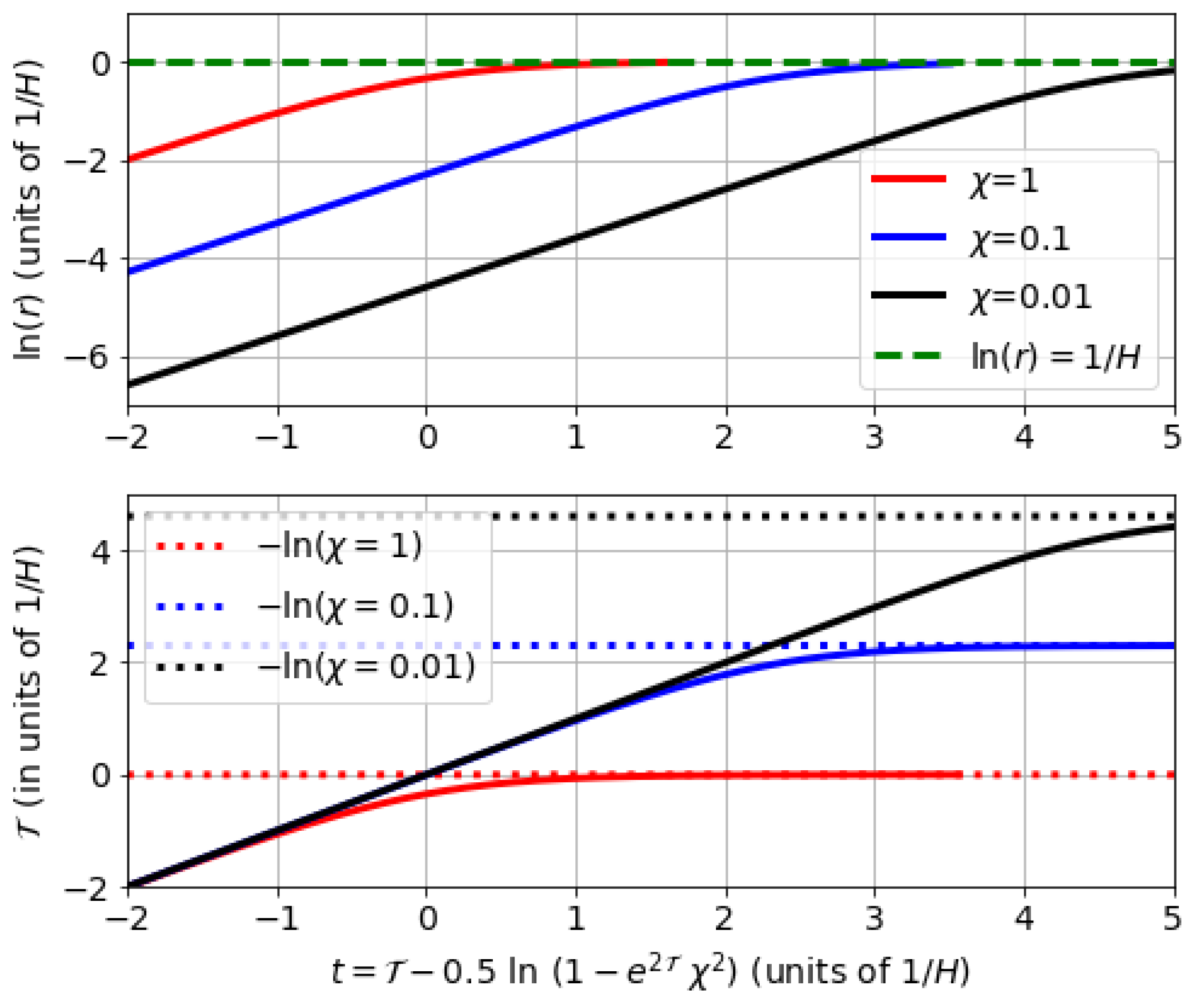
where and reproduces dS metric (see Ref. [80] for some additional discussion). In co-moving coordinates, the metric is inflating exponentially: , while in physical coordinates it is static. Figure A1 illustrates how this is possible and shows how freezes to a constant as (this is because shrinks to zero). Note also how in Equation (A17) for is the generalization of Equation (A20) for .
Consider a solution with spherical symmetry as in Equation (A5) where we have matter and radiation inside some radius R and empty space outside:
For uniform density inside this we should reproduce the FLRW solution for and the SBH solution for . This follows from Gauss law (or the corollary to Birkhoff’s theorem [16]) where each sphere collapses independent of what is outside . To see this more explicitly for the interior solution, we use the dSE notation in Equation (A16): , so that:
At the junction , we find that:
which matches Equations (15) and Equation (4). For a regular star so the expansion is subluminar because . Our Universe has (we observe super-horizon scales in the CMB), which, using Equation (A23), requires : i.e., we are inside our own BH! For we can change variables as in Equation (A17)–(A19). In the co-moving frame of Equation (A19), from every point inside the BHU, co-moving observers will have the illusion of an homogeneous and isotropic space-time around them, with a fixed Hubble–Lemaitre expansion . This converts the dSE metric into the FLRW metric. So the solution is and . Given and in the interior we can use Equation (3) to find and :
Figure A1.
Logarithm of physical radius (top) and co-moving time (bottom) as a function of Schwarzschild time t in Equation (A20) for and different values of . All quantities are in units of . For early time or small : . A fix acts like an Horizon: as we have (dotted), which freezes inflation to: (dashed).
This corresponds to a homogeneous FLRW* of fix energy-mass confined inside . The co-moving radius corresponding to R is . We can see how R can be related with a (free-fall) geodesic radial shell:
where . For a time-like geodesic of constant () we have and , which reproduces Equation (A23). For a null-like geodesic (): . The case corresponds to in Equation (32) from which we can immediately see that . So even when , the energy-mass M inside R generates (see also Section 2.2.2). We can integrate Equation (A25) to find , for a fix and , regardless of . This shows that a solution for exist for any content inside R. To complete the solution, i.e., to find and , we need to solve Equation (A17) with . For the solution is and Equation (A20). The FLRW metric with becomes the dS metric in Equation (A13). Such solutions are illustrated in Figure A2.
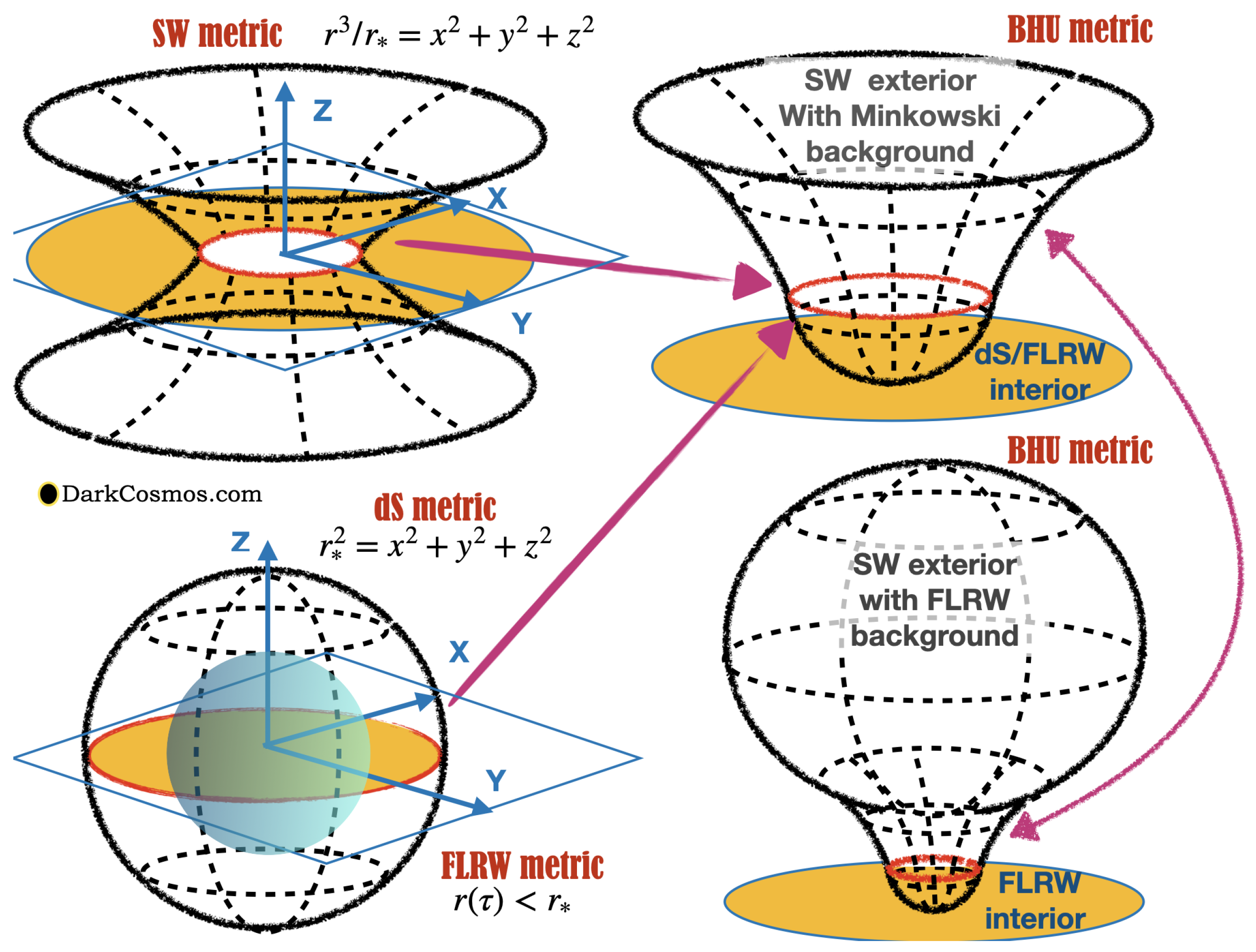
Figure A2.
Spatial representation of 2D metric embedded in 3D flat space for: deSitter (dS, bottom left, ), FLRW (, blue sphere inside dS), Schwarzschild (SW, top left, ) and two versions of the combined BHU metrics. The yellow region shows the projection coverage in the plane. In the top right figure we show a BHU with dS (or FLRW) interior and SBH metric exterior joint at the Event Horizon (red circles). The BHU solution has in general two nested FLRW metrics joined by the SBH metric (bottom right). See Appendix C for a more detailed explanation.
Appendix C. Geometrical Representations
To visualize the spatial BHU metric in a 2D plot we consider the most general shape for a spherically symmetric metric in 2D space embedded in 3D flat space (see also Section 7.1.3 in Ref. [9]). In polar coordinates with and we have:
In 3D space we just have one additional angle, , in Equation (A5), but the radial part is the same. The case corresponds to flat space: . The simplest case with curvature can be represented by a 2D sphere (S2) embedded in 3D flat space using an extra dimension z:
This metric is flat in 3D coordinates, but constrained to , which is the radius of the sphere and the curvature within the 2D surface of S2. We can replace z by r using: to find:
so that just like in the dS metric of Equation (A13) for . It tell us that dS space corresponds to being in the flat surface of a sphere (like us in Earth). This is illustrated in the bottom left of Figure A2. Note how are coordinates in the plane. The S2 space is trapped or bounded by (yellow region). The metric changes signature (becomes imaginary) for : this region cannot be reached (white region). The case (red circles) corresponds to the Event Horizon at .
The Newtonian interpretation of is that this is caused by a centrifugal force, like that in the orbit of a satellite. Even when there is no matter, the curvature (or boundary) is interpreted as a repulsive gravitational force that causes acceleration.
The FLRW metric (or dSE metric in Equation (A19)) corresponds to a smaller sphere S2 (inside dS sphere) with an expanding radius that tends asymptotically to (see Equation (A19)):
So, it has the same topology and Event Horizon or trapped surface (red circle) as the dS metric. It is represented in Figure A2 by a blue sphere inside dS sphere in the bottom left corner. This illustrates how it is possible that each observer inside sees an homogeneous space even when the sphere is centred around a given position.
The next simplest case can be represented by a static radius that increases with r, i.e.,: . We can replace z by r using: to find:
so that just like in the SBH metric of Equation (A12) for . This is illustrated in the top left of Figure A2. The case (red circle) corresponds to the Event Horizon at . The Newtonian interpretation for is the inverse square law for a point mass M: .
The Schwarzschild space is bounded by (yellow region). The metric changes signature (becomes imaginary) for and this region can not be reached. This coverage is complementary to the dS or FLRW metric, which only covers the inner region. We can match the dS and SBH metrics at to cover the full plane as in the BHU metric. Physically, this corresponds to a balance between the centrifugal force, represented by dS potential , and the SBH inverse square law, , like what happens in the circular Keplerian orbits. This matching is the junction in Equation (15) which corresponds to a causal boundary. This can also be seen as a Lorentz contraction where the velocity u is given by the Hubble–Lemaitre law: . The time duality between the FLRW and SBH frame can also be interpreted as a time dilation, see Equation (A19).
This BHU metric is shown in the top right of Figure A2, which is asymptotically Minkowski. The dS metric is the limiting case of FLRW metric and SBH metric is a perturbation over the FLRW metric. So, more generally, the BHU is a combination of 2 FLRW metrics joined by a SBH metric. The junction happens at the effective value of , which asymptotically tends to , corresponding to the inner FLRW. If the outer FLRW has a mass , then the SBH hyperbolic surface will close as another S2 sphere (bottom right panel) with .
Appendix D. The FLRM* Mass
Contrary to what happens in special relativity, in GR mass, M can not always be defined globally. This is the case for non asymptotically flat spaces, like dS or FLRW. Following Hayward [19], consider a spherically symmetric metric in the form:
with a perfect fluid inside. We recover units of to see the non relativistic limit. The FLRW case corresponds to and . The Misner and Sharp [10] energy-mass inside a spatial hypersurface , given by , is:
where is the 3D spatial volume element of the metric in . The first term corresponds to the material or passive mass (which we call here ):
We can then interpret the next two terms in the integrant of Equation (A32) as the contribution to M from the kinetic and potential energy. In the non relativistic limit, these two terms are negligible and . However, in general, as indicated by Equation (A32), can not be expressed as a sum of individual energies as also appears inside the integral, reflecting the non-linear nature of gravity.
In the FLRW metric we have , where , because and . For a co-moving observer we have: and using Equation (3): , so the last two terms cancel each other () and we find that , which we just call M as in Equation (4). For in Equation (32) we have that for small times (or small a) R is constant in co-moving coordinates, which means that . This is the case even when we have radiation and because the integral is dominated by for small a. Another way to understand this is to note that so that R is always causally disconnected, so there is no pressure at . This () is also the case in the dS phase because both and R become constant. However, there is an intermediate regime when we approach the dS phase where M reduces its value (). To understand this better, consider the FLRW solution to EFE, i.e., Equation (3):
We can see here how H tends to a constant () because , as expansion dilutes the energy content. So the mass for a co-moving observer in Equation (4) becomes:
as R approaches the BH radius , the density dilutes to zero (because of exponential expansion) and all that remains is the SBH mass: . So, the mass M for a co-moving observer M has two contributions: one from the kinetic energy of the expansion and one from the BH’s binding energy, . A physical (or Schwarzschild) observer outside only sees because is causally disconnected.
Mitra [80] noted that there is a contradiction in how global mass conservation is viewed by different coordinates in dS metric. Mitra pointed out that when the FLRW metric is dominated by , Equation (4) indicates that the mass is unbounded in co-moving coordinates because seems to grow unbounded with time, while H is constant. While in physical coordinates, the dS metric is static and therefore mass must be conserved. Part of the problem here is that the dS metric is not asymptotically flat and therefore mass is not well defined. We saw in Equation (32) that R is in fact bounded and argued that proper coordinates r and proper time , asymptotically freeze out for (see Figure A1). As is finite, M becomes constant if we only integrate inside R (i.e., in the FLRW* case). This agrees with both the outside static SBH metric and the inside asymptotically static dS metric. In other words, the FLRW* metric behaves better than the FLRW metric because it is asymptotically flat and has a well defined mass, as advocated by Friedmann–Lemaitre original cosmology (see Section 2.1).
References
- Ellis, G. Opposing the multiverse. Astron. Geophys. 2008, 49, 2.33–2.35. [Google Scholar] [CrossRef]
- Kormendy, J.; Ho, L.C. Coevolution (Or Not) of Supermassive Black Holes and Host Galaxies. ARAA 2013, 51, 511–653. [Google Scholar]
- Kusenko, A.E. Exploring Primordial Black Holes from the Multiverse with Optical Telescopes. PRL 2020, 125, 181304. [Google Scholar] [CrossRef] [PubMed]
- Buchdahl, H.A. General Relativistic Fluid Spheres. Phys. Rev. 1959, 116, 1027–1034. [Google Scholar] [CrossRef]
- Brustein, R.; Medved, A.J.M. Resisting collapse. PRD 2019, 99, 064019. [Google Scholar] [CrossRef]
- Mazur, P.O.; Mottola, E. Surface tension and negative pressure interior of a non-singular ‘black hole’. Class. Quantum Gravity 2015, 32, 215024. [Google Scholar] [CrossRef]
- Lemaître, G. Un Univers homogène de masse constante et de rayon croissant rendant compte de la vitesse radiale des nébuleuses extra-galactiques. Ann. Société Sci. Brux. 1927, 47, 49–59. [Google Scholar]
- Elizalde, E. The True Story of Modern Cosmology: Origins, Main Actors and Breakthroughs; Springer: Berlin/Heidelberg, Germany, 2021. [Google Scholar]
- Padmanabhan, T. Gravitation; Cambridge University Press: Cambridge, UK, 2010. [Google Scholar]
- Misner, C.W.; Sharp, D.H. Relativistic Equations for Adiabatic, Spherically Symmetric Gravitational Collapse. Phys. Rev. 1964, 136, 571. [Google Scholar] [CrossRef]
- Lemaître, G. Expansion of the universe, A homogeneous universe of constant mass and increasing radius accounting for the radial velocity of extra-galactic nebulae. MNRAS 1931, 91, 483–490. [Google Scholar] [CrossRef]
- Friedmann, A. Über die Krümmung des Raumes. Z. Phys. 1922, 10, 377–386. [Google Scholar]
- Friedmann, A. On the Curvature of Space. Gen. Relativ. Gravit. 1999, 31, 1991. [Google Scholar] [CrossRef]
- Tolman, R.C. Effect of Inhomogeneity on Cosmological Models. Proc. Natl. Acad. Sci. USA 1934, 20, 169–176. [Google Scholar] [PubMed]
- Oppenheimer, J.R.; Snyder, H. On Continued Gravitational Contraction. Phys. Rev. 1939, 56, 455–459. [Google Scholar] [CrossRef] [Green Version]
- Faraoni, V.; Atieh, F. Turning a Newtonian analogy for FLRW cosmology into a relativistic problem. PRD 2020, 102, 044020. [Google Scholar] [CrossRef]
- Johansen, N.; Ravndal, F. On the discovery of Birkhoff’s theorem. Gen. Relativ. Gravit. 2006, 38, 537–540. [Google Scholar]
- Vaidya, P.C. Nonstatic Analogs of Schwarzschild’s Interior Solution in General Relativity. Phys. Rev. 1968, 174, 1615–1619. [Google Scholar] [CrossRef]
- Hayward, S.A. Gravitational energy in spherical symmetry. Phys. Rev. D 1996, 53, 1938–1949. [Google Scholar]
- Faraoni, V.; Giusti, A.; Bean, T.F. Asymptotic flatness and Hawking quasilocal mass. PRD 2021, 103, 044026. [Google Scholar]
- Israel, W. Singular hypersurfaces and thin shells in general relativity. Nuovo Cimento B Ser. 1967, 48, 463. [Google Scholar]
- Barrabès, C.; Israel, W. Thin shells in general relativity and cosmology: The lightlike limit. PRD 1991, 43, 1129–1142. [Google Scholar] [CrossRef]
- Crisostomo, J.; Olea, R. Hamiltonian treatment of the gravitational collapse of thin shells. Phys. Rev. D 2004, 69, 104023. [Google Scholar] [CrossRef]
- Dodelson, S. Modern Cosmology; Academic Press: New York, NY, USA, 2003. [Google Scholar]
- Gaztañaga, E. The size of our causal Universe. MNRAS 2020, 494, 2766–2772. [Google Scholar] [CrossRef]
- Gaztañaga, E. The cosmological constant as a zero action boundary. MNRAS 2021, 502, 436–444. [Google Scholar]
- Parattu, K.; Chakraborty, S.; Majhi, B.R.; Padmanabhan, T. A boundary term for the gravitational action with null boundaries. Gen. Relativ. Gravit. 2016, 48, 94. [Google Scholar] [CrossRef]
- Ellis, G.F.R.; Rothman, T. Lost horizons. Am. J. Phys. 1993, 61, 883–893. [Google Scholar] [CrossRef]
- Melia, F. The apparent (gravitational) horizon in cosmology. Am. J. Phys. 2018, 86, 585–593. [Google Scholar]
- Kaloper, N.; Kleban, M.; Martin, D. McVittie’s legacy: Black holes in an expanding universe. PRD 2010, 81, 104044. [Google Scholar] [CrossRef]
- Pathria, R.K. The Universe as a Black Hole. Nature 1972, 240, 298–299. [Google Scholar] [CrossRef]
- Zhang, T.X. The Principles and Laws of Black Hole Universe. J. Mod. Phys. 2018, 9, 1838–1865. [Google Scholar] [CrossRef] [Green Version]
- Smolin, L. The Life of the Cosmos; Oxford University Press: Oxford, UK, 1997. [Google Scholar]
- Easson, D.A.; Brandenberger, R.H. Universe generation from black hole interiors. J. High Energy Phy. 2001, 2001, 024. [Google Scholar] [CrossRef]
- Daghigh, R.G.; Kapusta, J.I.; Hosotani, Y. False Vacuum Black Holes and Universes. arXiv 2000, arXiv:gr-qc/0008006. [Google Scholar]
- Firouzjahi, H. Primordial Universe Inside the Black Hole and Inflation. arXiv 2016, arXiv:1610.03767. [Google Scholar]
- Oshita, N.; Yokoyama, J. Creation of an inflationary universe out of a black hole. Phys. Lett. B 2018, 785, 197–200. [Google Scholar] [CrossRef]
- Dymnikova, I. Universes Inside a Black Hole with the de Sitter Interior. Universe 2019, 5, 111. [Google Scholar] [CrossRef]
- Grøn, Ø.; Soleng, H.H. Dynamical instability of the González-Díaz black hole model. Phys. Lett. A 1989, 138, 89–94. [Google Scholar] [CrossRef]
- Blau, S.K.; Guendelman, E.I.; Guth, A.H. Dynamics of false-vacuum bubbles. PRD 1987, 35, 1747–1766. [Google Scholar] [CrossRef]
- Frolov, V.P.; Markov, M.A.; Mukhanov, V.F. Through a black hole into a new universe? Phys Lett. B 1989, 216, 272–276. [Google Scholar] [CrossRef]
- Aguirre, A.; Johnson, M.C. Dynamics and instability of false vacuum bubbles. PRD 2005, 72, 103525. [Google Scholar] [CrossRef]
- Garriga, J.; Vilenkin, A.; Zhang, J. Black holes and the multiverse. JCAP 2016, 2016, 064. [Google Scholar] [CrossRef]
- Gonzalez-Diaz, P.F. The space-time metric inside a black hole. Nuovo Cimento Lett. 1981, 32, 161–163. [Google Scholar] [CrossRef]
- Shen, W.; Zhu, S.T. Junction conditions on null hypersurface. Phys. Lett. A 1988, 126, 229–232. [Google Scholar]
- Poisson, E.; Israel, W. Structure of the black hole nucleus. Class. Quantum Gravity 1988, 5, L201–L205. [Google Scholar] [CrossRef]
- Penrose, R. Gravitational Collapse and Space-Time Singularities. Phys. Rev. Lett. 1965, 14, 57–59. [Google Scholar] [CrossRef]
- Dadhich, N. Singularity: Raychaudhuri equation once again. Pramana 2007, 69, 23. [Google Scholar] [CrossRef]
- Good, I.J. Chinese universes. Phys. Today 1972, 25, 15. [Google Scholar] [CrossRef]
- Knutsen, H. The idea of the universe as a black hole revisited. Gravit. Cosmol. 2009, 15, 273–277. [Google Scholar] [CrossRef]
- Stuckey, W.M. The observable universe inside a black hole. Am. J. Phys. 1994, 62, 788–795. [Google Scholar] [CrossRef]
- Popławski, N. Universe in a Black Hole in Einstein-Cartan Gravity. ApJ 2016, 832, 96. [Google Scholar] [CrossRef]
- Secrest, N.J.; von Hausegger, S.; Rameez, M.; Mohayaee, R.; Sarkar, S.; Colin, J. A Test of the Cosmological Principle with Quasars. ApJL 2021, 908, L51. [Google Scholar] [CrossRef]
- Moss, A.; Zibin, J.P.; Scott, D. Precision cosmology defeats void models for acceleration. Phys. Rev. D 2011, 83, 103515. [Google Scholar] [CrossRef]
- Fosalba, P.; Gaztañaga, E. Explaining cosmological anisotropy: Evidence for causal horizons from CMB data. MNRAS 2021, 504, 5840–5862. [Google Scholar] [CrossRef]
- Gaztañaga, E.; Fosalba, P. A peek outside our Universe. Symmetry 2022, 14, 285. [Google Scholar] [CrossRef]
- Yeung, S.; Chu, M.C. Directional Variations of Cosmological Parameters from the Planck CMB Data. arXiv 2022, arXiv:2201.03799. [Google Scholar] [CrossRef]
- Camacho, B.; Gaztañaga, E. A measurement of the scale of homogeneity in the Early Universe. arXiv 2021, arXiv:2106.14303. [Google Scholar]
- Gaztañaga, E. How the Big Bang Ends up Inside a Black Hole. Universe 2022, 8, 257. [Google Scholar] [CrossRef]
- Gaztanaga, E.; Camacho-Quevedo, B. Super-Horizon modes and cosmic expansion. arXiv 2022, arXiv:astro-ph.CO/2204.10728. [Google Scholar]
- Abdalla, E.; Abellán, G.F.; Aboubrahim, A.; Agnello, A.; Akarsu, Ö.; Akrami, Y.; Pettorino, V. Cosmology Intertwined: A Review of the Particle Physics, Astrophysics, and Cosmology Associated with the Cosmological Tensions and Anomalies. arXiv 2022, arXiv:2203.06142. [Google Scholar]
- O’Raifeartaigh, C.; Mitton, S. A new perspective on steady-state cosmology. arXiv 2015, arXiv:1506.01651. [Google Scholar]
- Bondi, H.; Gold, T. The Steady-State Theory of the Expanding Universe. MNRAS 1948, 108, 252. [Google Scholar] [CrossRef]
- Hoyle, F. A New Model for the Expanding Universe. MNRAS 1948, 108, 372. [Google Scholar] [CrossRef]
- Gaztañaga, E. Inside a Black Hole: The Illusion of a Big Bang. 2020. Available online: https://hal.archives-ouvertes.fr/hal-03106344 (accessed on 11 January 2021).
- Gaztañaga, E. The Black Hole Universe (BHU) from a FLRW Cloud. 2021. Available online: https://hal.archives-ouvertes.fr/hal-03344159 (accessed on 14 September 2021).
- Gaztañaga, E. The Cosmological Constant as Event Horizon. Symmetry 2022, 14, 300. [Google Scholar]
- Hilbert, D. Die Grundlage der Physick. Konigl. Gesell. D. Wiss. Göttingen Math-Phys K 1915, 3, 395–407. [Google Scholar]
- Weinberg, S. Gravitation and Cosmology; John Wiley & Sons: Hoboken, NJ, USA, 1972. [Google Scholar]
- Weinberg, S. Cosmology; Oxford University Press: Oxford, UK, 2008. [Google Scholar]
- Einstein, A. Die Grundlage der allgemeinen Relativitätstheorie. Ann. Der Phys. 1916, 354, 769–822. [Google Scholar]
- Landau, L.D.; Lifshitz, E.M. The Classical Theory of Fields; Elsevier: Amsterdam, The Netherlands, 1971. [Google Scholar]
- Carroll, S.M. Spacetime and Geometry; Addison-Wesley: Boston, MA, USA, 2004. [Google Scholar]
- York, J.W. Role of Conformal Three-Geometry in the Dynamics of Gravitation. PRL 1972, 28, 1082–1085. [Google Scholar]
- Gibbons, G.W.; Hawking, S.W. Cosmological event horizons, thermodynamics, and particle creation. PRD 1977, 15, 2738–2751. [Google Scholar]
- Hawking, S.W.; Horowitz, G.T. The gravitational Hamiltonian, action, entropy and surface terms. Cl. Quantum Gravity 1996, 13, 1487. [Google Scholar] [CrossRef]
- Tolman, R.C. Relativity, Thermodynamics, and Cosmology; Dover Publications: New York, NY, USA, 1934. [Google Scholar]
- Diez-Tejedor, A.; Feinstein, A. Homogeneous scalar field the wet dark sides of the universe. PRD 2006, 74, 023530. [Google Scholar] [CrossRef]
- Lanczos, K. Bemerkung zur de Sitterschen Welt. Phys. Z. 1922, 23, 539–543. [Google Scholar]
- Mitra, A. Interpretational conflicts between the static and non-static forms of the de Sitter metric. Nat. Sci. Rep. 2012, 2, 923. [Google Scholar] [CrossRef] [Green Version]
- Lanczos, K.; Hoenselaers, C. On a Stationary Cosmology in the Sense of Einstein’s Theory of Gravitation [1923]. GR Gravit. 1997, 29, 361–399. [Google Scholar]
Figure 1.
Illustration of the BHU inside the event horizon GM. This is a Schwarzschild (empty) metric outside () and a FLRW metric with a Hubble radius inside (). The BHU solution in Equation (15) requires . This means that there is a region with matter outside the Hubble radius (yellow shading, see also Figure 2).
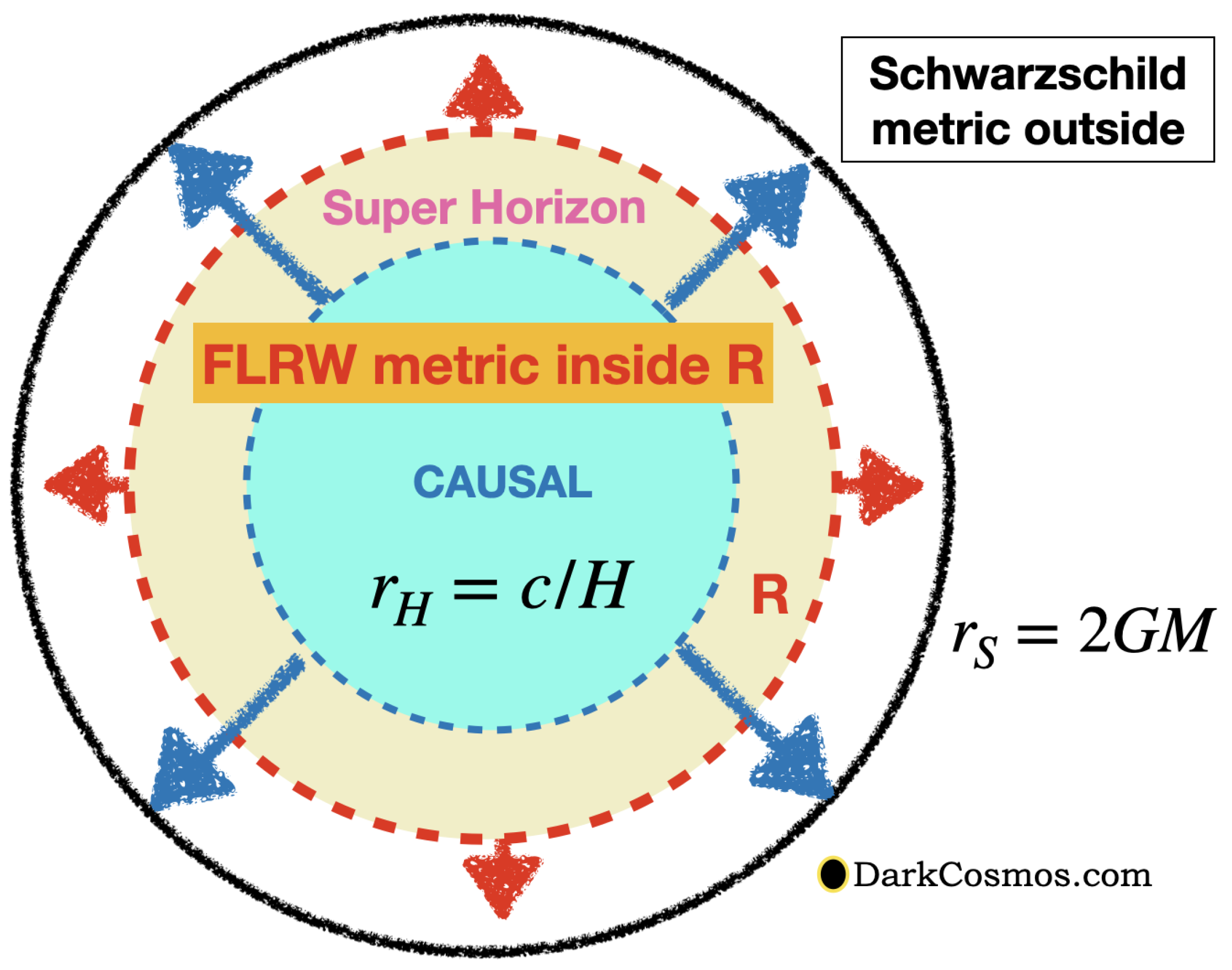
Figure 3.
Same as Figure 2 in co-moving coordinates (linear scale). The two dashed green lines are the past-line cones for an observer at the centre (lower line) or off centred (upper line). The difference between the FLRW event horizon and is constant in co-moving coordinates (see Equation (35)). This is why all observers within R today see the same homogeneous background and cannot observe photons with anytime in their past light-cone.

Publisher’s Note: MDPI stays neutral with regard to jurisdictional claims in published maps and institutional affiliations. |
© 2022 by the author. Licensee MDPI, Basel, Switzerland. This article is an open access article distributed under the terms and conditions of the Creative Commons Attribution (CC BY) license (https://creativecommons.org/licenses/by/4.0/).
Share and Cite
MDPI and ACS Style
Gaztanaga, E. The Black Hole Universe, Part I. Symmetry 2022, 14, 1849. https://doi.org/10.3390/sym14091849
AMA Style
Gaztanaga E. The Black Hole Universe, Part I. Symmetry. 2022; 14(9):1849. https://doi.org/10.3390/sym14091849
Chicago/Turabian StyleGaztanaga, Enrique. 2022. "The Black Hole Universe, Part I" Symmetry 14, no. 9: 1849. https://doi.org/10.3390/sym14091849
Note that from the first issue of 2016, this journal uses article numbers instead of page numbers. See further details here.