

The Black Hole Universe, Part II


1
Institute of Space Sciences (ICE, CSIC), 08193 Barcelona, Spain
2
Institut d Estudis Espacials de Catalunya (IEEC), 08034 Barcelona, Spain
Symmetry 2022, 14(10), 1984; https://doi.org/10.3390/sym14101984
Submission received: 31 August 2022
/
Revised: 19 September 2022
/
Accepted: 20 September 2022
/
Published: 22 September 2022
(This article belongs to the Special Issue Nature and Origin of Dark Matter and Dark Energy)
Abstract
In part I of this series, we showed that the observed Universe can be modeled as a local Black Hole of fixed mass , without Dark Energy: cosmic acceleration is caused by the Black Hole event horizon rS = 2GM. Here, we propose that such Black Hole Universe (together with smaller primordial Black Holes) could form from the hierarchical free-fall collapse of regular matter. We argue that the singularity could be avoided with a Big Bounce explosion, which results from neutron degeneracy pressure (Pauli exclusion principle). This happens at GeV energies, like in core collapse supernova, well before the collapse reaches Planck energies (1019 GeV). If our Universe formed this way, there is no need for Cosmic Inflation or a singular start (the Big Bang). Nucleosynthesis and recombination follow a hot expansion, as in the standard model, but cosmological measurements (which are free parameters in the standard model) could in principle be predicted from first principles. Part or all of the Dark Matter could be made up of primordial compact objects (Black Holes and Neutron Stars), remnants of the collapse and bounce. This can provide a faster start for galaxy formation. We present a simple prediction to explain the observed value of or equivalently (the fraction of the critical energy density observed today in form of Dark Energy) and the coincidence problem .
1. Introduction
A cosmological model predicts the background evolution, composition and structure of the observed Universe given some initial conditions. The standard cosmological model [1,2], also called CDM, assumes that our Universe began in a hot Big Bang (BB) expansion at the very beginning of space-time. Such initial conditions seem to violate the classical concept of energy conservation and are very unlikely [3,4,5,6]. Our observed Hubble Horizon has a total mass energy closed to in the form of stars, gas, dust and Dark Matter, which according to the singular start BB model came out of (macroscopic) nothing in the form of some quantum gravity vacuum fluctuations that we can only speculate about and we will never be able to test experimentally because of the enormous energies involved ( GeV). There is no direct evidence that this ever occurred. This model also requires three more exotic ingredients or patches: Cosmic Inflation, Dark Matter and Dark Energy (DE), for which we have no direct evidence or understanding at any fundamental level. Another problem of the CDM model is why the value of (or DE) is such that ∼ today: the cosmological coincidence problem (see [1,2,7,8]). Despite these shortfalls, the CDM model seems very successful in explaining most observations by fitting just a handful of free cosmological parameters.
In reference [9] (paper I, from now on), we propose a new cosmological solution, the Black Hole (BH) Universe (BHU) that can explain the same observations as CDM without the need of Dark Energy (which is just the BHs event horizon). This solution can also be used to model the interior of regular BHs. However, it is not enough to find a new solution to GR. We need to make sure that such a configuration can be achieved in a causal way. A good example of this problem is the infinite Friedman–Lemaitre–Robertson–Walker (FLRW) solution. The Hubble rate is the same everywhere, no matter how far, and this is not causally possible [10,11]. Cosmic Inflation alleviates this problem but does not solve it [6]. We propose two possible BHU formation scenarios: (i) one that happens during a rapid expansion (or explosion) and (ii) a version that happens during a free-fall collapse. Both can be applied to a small object, such as a star, or a large object, such as our Universe. The main difference is that for the larger object, the density corresponding to is very low (few atoms per cubic meter), and we can assume a dust () fluid. This is not the case for small objects, such as stars.
In the appendix, we present the expanding scenario, which requires an existing expansion (such as Cosmic Inflation or a supernova explosion) and a scalar field in a false vacuum potential. This also means that the outside manifold has a different effective term (the true vacuum) and will not be asymptotically flat. So, this shares many of the problems of the standard CDM model that we are trying to avoid, resulting in a more complicated and speculative scenario. Thus, we focus on the hierarchical free-fall collapse to form a BHU, as presented in Section 2, which can start from a uniform low-density cloud of regular matter. Section 3 presents a new anthropic argument to predict the observed value for our BHU mass M and cosmic acceleration. Finally, Section 4 is devoted to our conclusions and discussions.
2. BHU Collapse
BHs are thought to form from gravitation collapse. So, we will study next a simple but generic collapse scenario for pressureless matter.
2.1. FLRW Cloud Collapse
Consider a uniform spherical cloud of dust or CDM (that is, an energy density with pressure ) with radius R and mass M, surrounded by a region that can be approximated as empty space. The cloud composition is not important to start with, but it could play some role later on. You can imagine an infinite uniform FLRW universe with a very low density, filled with small random amplitude fluctuations of different sizes. The Hubble rate will be close to zero as in empty Minkowski space. We will focus on one particular positive random fluctuation that slowly collapses, forming a cloud of size R.
Such a cloud will collapse following the FLRW* solution in GR (see paper I). The solution is exactly the same in Newtonian physics [12]. The radius r inside R () is given by , where is a fixed comoving coordinate. The rate of collapse is given by the Hubble–Lemaitre law:
At any time (this is proper time for a comoving observer), the collapse rate H is given by the energy density . During collapse, energy–mass conservation requires that . Given and at time , this equation can be integrated with solution:
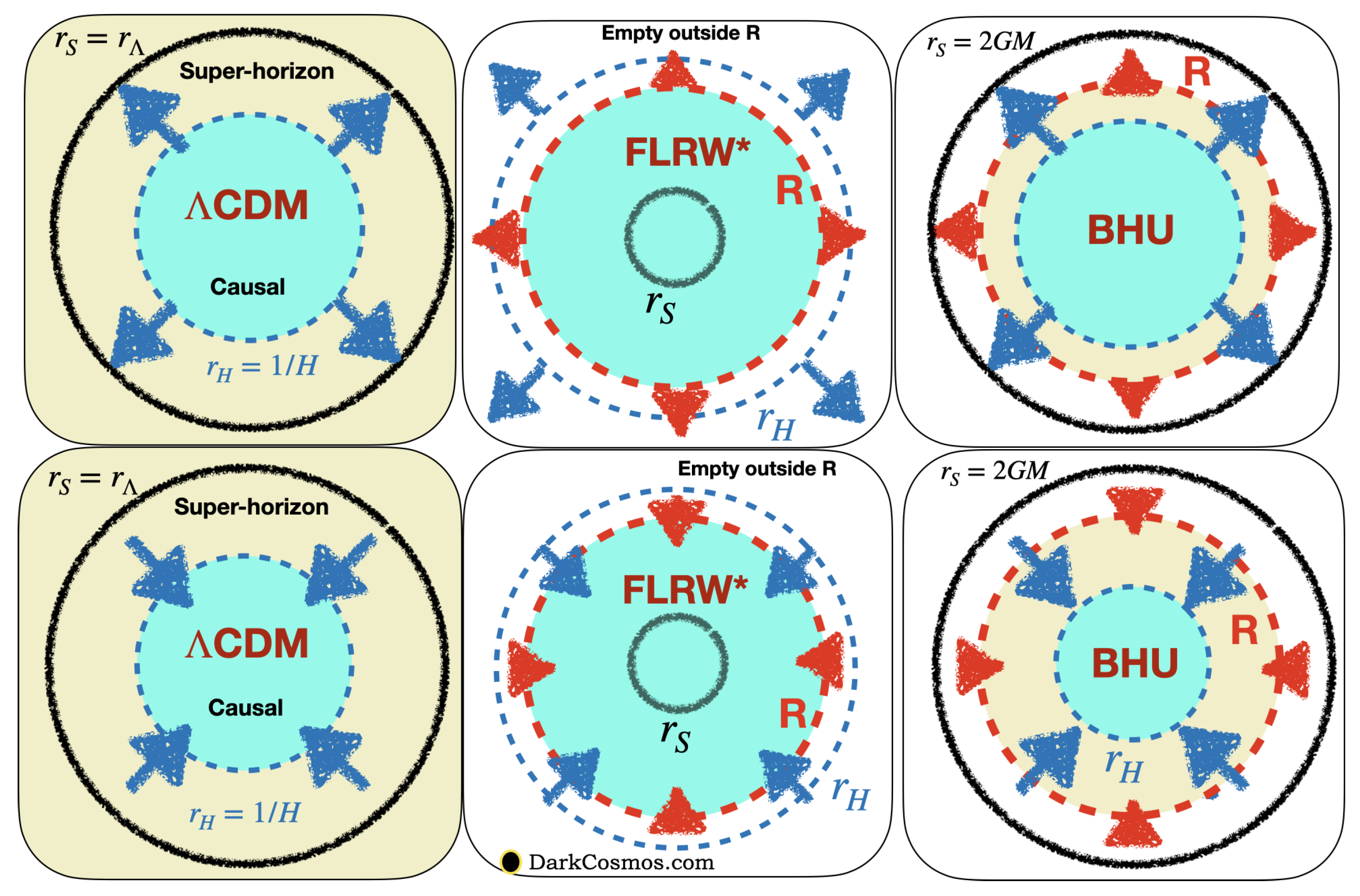
During collapse, H and are negative. Note also that during collapse , but we will refer to its absolute value to compare to the radial coordinate r. As proper time approaches the singularity (at ), becomes smaller and becomes larger. Structures that are larger than cannot evolve because the time that a perturbation takes to travel that distance is larger than the expansion time. This is illustrated in Figure 1.
The mass M inside R in the FLRW* cloud is (see paper I for details) is:
so that:
So, we can see that as , we have and . Before collapsing into a BH (i.e., ) we have that . After BH collapse: (see Figure 1).
Once you form a BH, the collapsed time (i.e., time before singularity) is quite short:
The mean energy density of a BH (as measured by an observer outside in flat empty space) at is:
regardless of its content. This agrees with Equation (1) for , indicating that the collapse eventually produces a BH and keeps growing inside the BH. This of course neglects preassure or rotation.
This critical value should be compared with the atomic nuclear saturation density:
which corresponds to the density of heavy nuclei and results from the Pauli exclusion principle applied to neutrons and protons. For a Neutron Star (NS) with , both densities are the same: . This relation indicates that it is difficult to form BHs from gravitational collapse with masses smaller than , because you somehow need to first overcome the Pauli exclusion principle. It also explains why NS are never larger than , as a collapsing cloud with such mass reaches BH density before it reaches . The maximum observed M for NS is closer to [13], which agrees with more detailed considerations that include the equation of state estimates. Cold nuclear matter at neutron density is a major unsolved problem in modern physics [13]. Fortunately, we should be able to understand this better in the near future with further modeling (see e.g., [14]) and pulsar and NS observations. This issue could be critical to understand cosmic expansion, as we will discuss here later in Section 2.3.
2.2. Hierarchical or Self Similar Collapse
Imagine a very large (or infinite) and uniform (FLRW) space-time with an initially Gaussian distribution of small random fluctuations , so that . Let us further assume that the amplitude of fluctuations is similar on all scales. By its definition, gravity dominates for masses above the Jeans mass . For such masses, we can apply the simple free-fall gravitational collapse presented in the subsection above. The positive fluctuations with the smallest masses will collapse first and form a BH for or an NS for smaller masses. Larger scales will collapse later and will be made of a uniform mix of already collapsed BH, NS, and background matter. The largest scale perturbations, corresponding to the largest masses, will collapse last.
We do not know the initial particle composition of this low-density fluid, but we can assume that it is similar to the one in our Universe. The density is so low that BHs will behave like collisionless dark matter (CDM). The hierarchical gravitational collapse could also lead to dense cold dark matter (CDM) halos and not necessarily to collapsing BHs. This is the case even if the CDM that we observe today is not made of new exotic DM particles but is made of compact objects with regular matter (such as BHs and NSs). Massive BHs could still form inside CDM halos. So, compact objects could correspond to halos with BHs inside or just naked BHs or NSs.
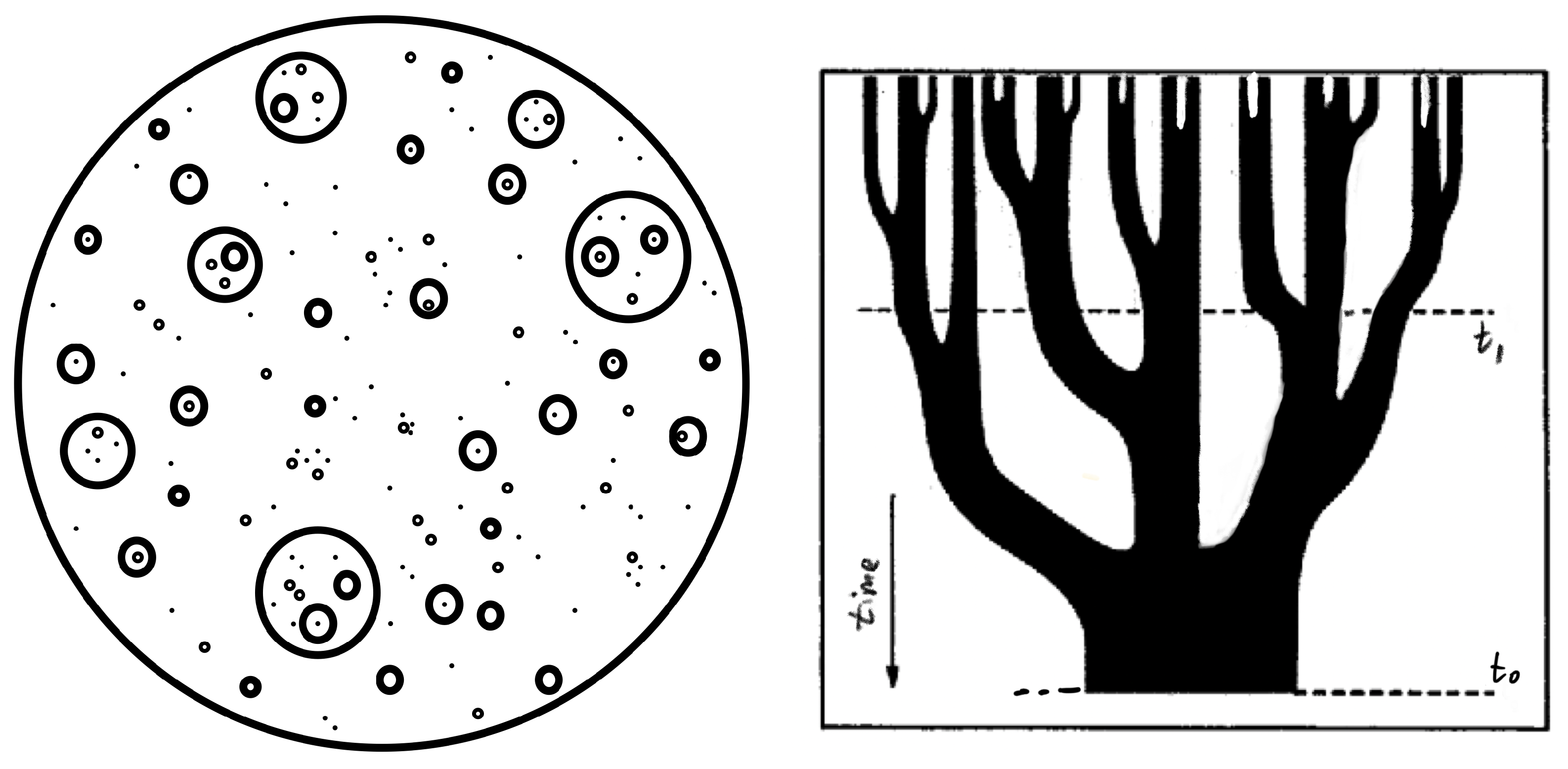
This leave us with a hierarchical picture, as illustrated in Figure 2, of small BHs inside larger naked BHs or DM halos. Only the smallest BHs will have NSs inside and, as we will see next, only the very large BHs will contain stars and galaxies inside. As we will see later in Section 3, for a Gaussian distribution, we can calculate the probability of structures of different M to form. All this is a crude approximation, as we are neglecting deviations from spherical symmetry and rotation, but it gives us a good idea of how hierarchical formation works [15].
These ideas has been tested in a more realistic way using cosmological N-body simulations (e.g., see [16] and references therein). Note that recent large scale N-body studies are mostly completed in an expanding (and not collapsing) background, which is dominated by (as it happens in our Universe today). In this case, the hierarchy is truncated for the largest objects (, see Section 3 below) because there is not enough time for larger compact objects to form (as structure freeze out during the deSitter (dS) phase of the expansion, i.e., close to now). Early N-body simulation without show a much more scale-free hierarchy without truncation (e.g., see [17] and references therein). We expect that this will be even more pronounced when the background is collapsing (instead of expanding) because gravity works in the same direction as collapse.
Typically, once a BH is formed, the internal collapse time in Equation (5) is quite short, and no further structures can form inside. The astronomical time needed to form a star similar to our Sun is measured in units of Gyr or yr. This means that according to Equation (5), to form a star similar to our Sun inside a BH, it has to be a very large one: . This is the mass inside our FLRW event horizon (for details, see paper I). Such a large BHU has a very low density, , which is 25% lower than the critical density today (a few protons per cubic meter).
According to the equations above, each of the hierarhical BHs collapses into a singularity. However, as mentioned before, quantum mechanics does not allow for matter to become singular. Well before we reach Planck scales ( GeV), we encounter nuclear saturation in Equation (7) (1 GeV). Although we cannot observe from outside what happens inside, it is reasonable to expect that the collapse will bounce into an explosion, as it happens in core collapse supernovae. The difference with a regular core collapse is that we are inside a BH. During expansion, the action is bounded by the BH event horizon, and the expansion turns into a dS phase, which corresponds to an asymptotically static BHs in proper coordinates (see paper I). So, the collapsing hierarchy is not quite symmetric with the expanding hierarchy. However, there is one case where we can actually observe what happens inside: our own BHU.
2.3. The Big Bounce
From the previous considerations, we conclude that our observed Universe could have formed from the collapse of a very large FLRW cloud. However, when we measured the Hubble–Lemaitre law, we observe expansion () and not collapse (). This means that we must have gone through a Big Bounce sometime in our past. Such a Big Bounce then replaces the role of the hot Big Bang (BB), which requires either Inflation or a singular start. Here are some ideas as to how this Big Bounce could have happened:
(1) Our local FLRW cloud must first collapse to form a BH. Before it collapses, the density of such a large cloud was so small that radiation escaped the cloud, so that . Radial comoving shells of matter are in free-fall collapse and continuously pass inside its own BH horizon. We take in Equation (2) as the time () when , i.e., when the BH forms (). Collapse and expansion are not symmetric because the event horizon is not symmetric: it allows matter to fall in but not to get out. This is key to the BHU model. We then find that the BH forms at time :
i.e., before (the BB) or 25 Gyr ago (when we add 14 Gyr from the BB to now).
(2) The collapse continues inside until it reaches nuclear saturation in Equation (7). The Hubble radius corresponding to Equation (7) is only 21 km and contains 7 . So, the collapse mass and scale is similar to that in the interior of a regular collapsing star. Typical supernova explosion energy accounts for a significant fraction of the progenitor rest mass. So, to explain the formation of the typical NS with 1–3 that we observed in nature, we would need a large progenitor (3–9). These values are closed to the 7 obtained from comparing Equation (7) with Equation (6), indicating that neutron degeneracy pressure will have some role in the collapse of the Hubble horizon region. Higher densities cannot be reached because of the Pauli exclusion principle. This indicates that the collapse must be halted by neutron degeneracy pressure, causing the implosion to rebound as it happens in stars [18]. Other bouncing mechanisms have been proposed [19,20,21], but they assume modifications to Classical GR. The CPT-Symmetric Universe idea [22,23] could provide an alternative bouncing mechanism.
(3) The different Hubble size regions within the BHU explode in sync because (ignoring smaller scale fluctuations) the background density is approximately the same everywhere in the collapsing FLRW cloud. The collapse energy () bounces into approximately uniformed expansion (). Radiation, baryons, NSs and primordial Black Holes (PBHs) result from each Hubble size region as compact remnants that can make up all or part of Dark Matter . Such compact remnants do not necessarily disrupt Nucleosynthesis or CMB recombination as long as they are not too large [24,25]. The bounce must produce the right amount of diffuse baryons per photon () so that Nucleosynthesis generates the observed primordial element abundance [26]. This will also give the right temperature for the observed CMB recombination physics.
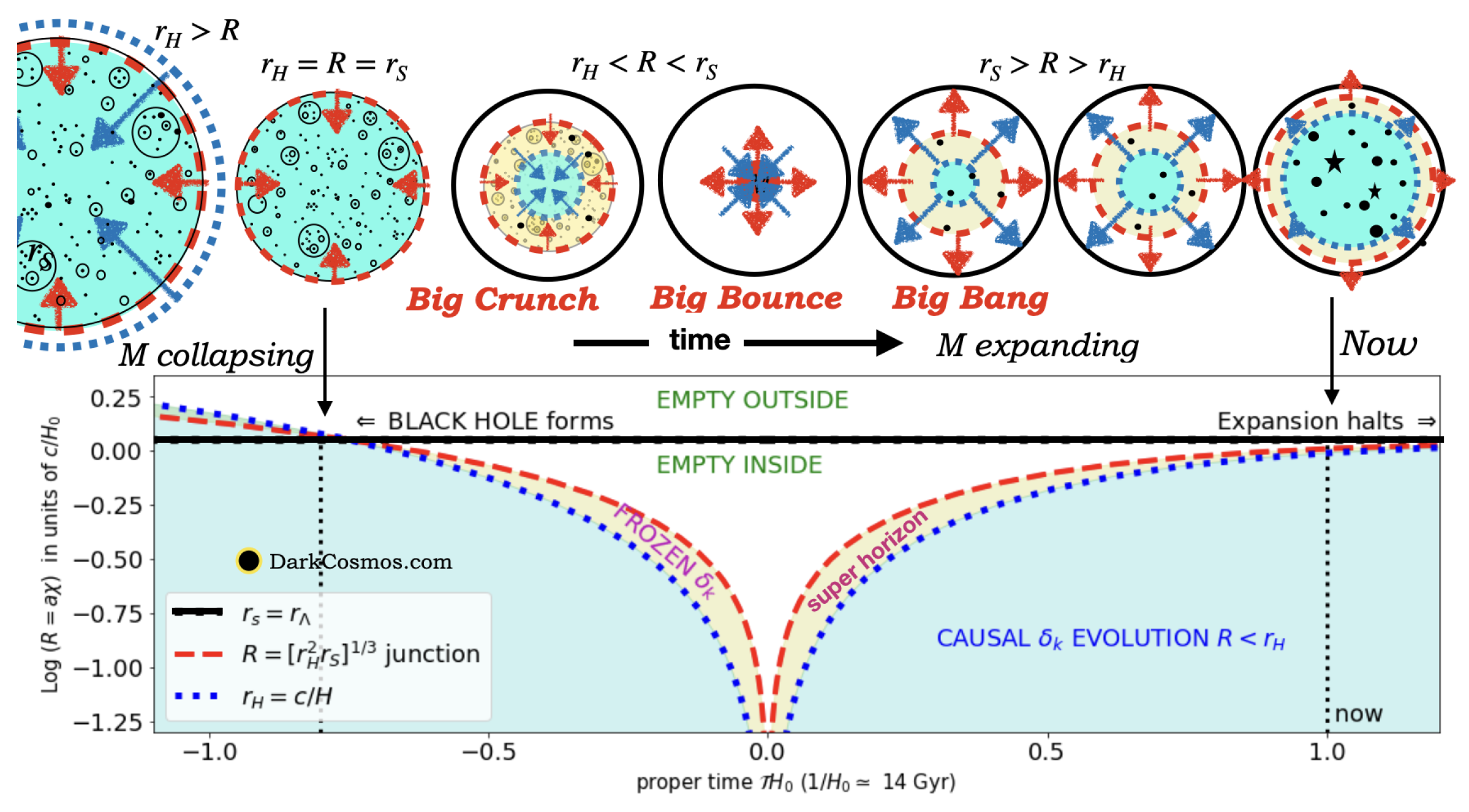
The top panel of Figure 3 illustrates this formation process. The bottom panel of Figure 3 shows an actual numerical calculation for the formation of our Universe. During collapse, the boundary R (falling red dashed line) is fixed in comoving coordinates and follows , where we have fixed to its observed value today with and is just given by Equation (1) with and . After the Big Bounce, R follows a null geodesic (rising red dashed line) with given by effective and . The Big Bang happened Gyrs ago, and our Universe collapsed into a BH about 25 Gyrs ago.
2.4. Comparison with Inflation
Inflation [27,28,29,30] is a key ingredient in the standard CDM cosmological model. For a review, see [1,31]. It solves several problems; the most relevant here are: (1) the horizon problem, (2) the source of Large-Scale Structure (LSS), (3) the flatness problem, and (4) the monopole problem. The horizon and LSS problems rise because much of the LSS that we observed today, e.g., BAO in CMB maps, was outside the Hubble Horizon at the time of light emission and therefore could not have had a causal origin. The idea of inflation is that during the very first instances of the Big Bang, the Universe became dominated by some FV or DE, which produced a dS expansion phase (see also our Appendix). Such an exponential expansion solves all the above problems. After expanding by a factor , Inflation leaves the universe empty, and we need a mechanism to stop Inflation and to create the matter and radiation that we observe today. This is called re-heating. These require fine-tuning and free parameters that we do not understand at a fundamental level. Inflation is not directly observable or testable, because it occurred when the Universe was opaque and at energies ( GeV) that are out of reach in particle accelerators [1]. Another problem of the CDM model that is not solved by Inflation is why there is DE or , and why the value of is such that today: the cosmological coincidence problem (see [1,2,7,8]).
As detailed before, a large fraction of the mass M that collapsed into our BHU is outside , especially close to singular time (), as (see Figure 1 and Figure 3). This clearly solves the horizon problem. Perturbations can be generated during the collapse and exit the horizon before the Big Bounce. Such super-horizon perturbations translate into inhomogeneities in the Big Bounce and can be the source of LSS structures when they re-enter during expansion. Long before Inflation was invented, Harrison [32], Zel’dovich [33] and Peebles [34] proposed that the gravitational instability of regular matter alone can generate a scale-invariant spectrum of fluctuations, which is very similar to the predicted in models of Inflation. This means that both models (Inflation or the BHU) could make similar predictions.
Inflation speculates that reheating could produce the right number of baryons per photon () needed for Nucleosynthesis and CMB recombination. The simplest models of Inflation also predict adiabatic scale-invariant fluctuations (given by an overall amplitude and slope ) in agreement with current observations [1]. However, note that the actual parameters that are fitted to observations (∼, ∼1, ∼, or ∼4) are not fundamental predictions of Inflation but rather free parameters of the CDM model.
In the BHU, the Big Bounce replaces the role of reheating and gives rise to (diffused baryons to photons) and (compact to diffused baryons). The collapse and bounce can also generate the initial spectrum of fluctuations needed to explain the observed cosmic structures (∼ and ∼1). Gravitational instability [32,33,34] allows perturbations to grow causally during the collapse phase, but they quickly exit as the collapse approaches . Such causally disconnected regions will therefore have slightly different and at the time close to the Big Bounce ( s). These regions correspond to super-horizon perturbations in the CMB that re-enter during the expansion given rise to the structures that we see today in Cosmic Maps.
Because R is always finite, we expect a cut-off in the spectrum of perturbations. This is at odds with the simplest prediction of Inflation. Recent anomalies in measurements of cosmological parameters over very large super-horizon scales agree better with the BHU predictions than with Inflation [35] and indicate that large super horizon fluctuations are not adiabatic, which is in contrast to what is predicted by Inflation. This again could provide evidence for the Big Bounce, which is an out of equilibrium process and cannot be modeled as a perfect fluid or an adiabatic process. Other differences include the abundance of primordial compact remnants, which could made up DM, speed up galaxy formation and produce an intrinsic CMB dipole (see discussion).
The BHU Big Bounce model is speculative in the same way Inflation is speculative. The main difference is that Inflation happens at energies that we will never be able to test, whereas the Big Bounce collapse within the BHU can be modeled and tested using the same Nuclear Astrophysics (and observations) that are used to understand Neutron Stars, Pulsars or core collapsed Supernovae. Further work is needed to show this in detail. This new model has the potential to explain from first principles some key cosmological observations, such as , , or , which are currently fixed by observations as free parameters of the CDM model (see Table 1 for a detailed comparison).
2.5. Why Is the Universe Flat?
So, if inflation did not happen, why is our Universe flat? The results in paper I can be applied to a FLRW cloud with if we just redefine:
so this does not change our BHU model or interpretation. A time-like geodesic of constant comoving radius contains a constant mass M also for . However, what is the motivation to choose a particular topology, other than that of empty space ()? The so-called “flatness problem”, that is solved by Inflation, is only a problem if you assume that the Big Bang Planck singularity (or the postulated initial conditions) will produce different values for the topological curvature k. The same can be argued about a global term. The field equations of GR are local, and they do not change k or by the presence of matter. These are global topological quantities imposed as the starting point to the equations. So, any choice other than would require some justification that is outside GR. In our analysis, we just assumed the most simple topology, that of empty space with , because we do not start from a past Planck singularity but from almost empty Minkowski space (before the BHU collapse). In the subsequent BHU evolution, k or remain zero, and the singularity is avoided at GeV, well before Quantum Gravity effects ( GeV), so we do not expect monopoles, a global curvature or to emerge.
3. The Apollonian Universe
Whatever the formation mechanism, one could ask: what was there before our BHU formed? We will assume here that there are other BHUs and regular matter within a larger space-time that we call the Apollonian Universe. Above the Jeans mass , we can use the Press–Schechter formalism [15] to predict the number of collapsed objects of a given mass M. For a scale-free power spectrum (scalar spectral index ) close to the one inside our BHU at the largest scales:
where corresponds to the gravitational collapse non-linear transition scale. More generally, for different spectral indexes n, we have . This result can be understood as the abundace of peaks in a Gaussian field [36]. The important point to notice is that large collapsed objects are exponentially suppressed for . The typical value of increases with time. The value today corresponds to a cluster mass: but was lower in the past. In our observed expanding Universe (inside now), we do not expect objects above to form in the future because structure formation freezes out during the dS phase (), but this is not a limit for the exterior background where the BHU collapsed because (see Section 2.5).
We assume that the probability of having observers like us increases linearly with time for and is zero for . So, is the astronomical time needed for observers like us to exist. Its value must be close to Gyrs, corresponding to the age of our galaxy [37], which is only about three times the age of our planet: Gyr [38]. The BH collapse time in Equation (5) is proportional to M, so that a large mass in Equation (3) has a typical collapse time of Gyr in Equation (5) (i.e., Equation (8)). The expansion time is longer because of the acceleration caused by the BH event horizon, but during the de-Sitter phase, the Hubble Horizon shrinks and structure formation halts. So, in practice, the relevant timescale is the one given by matter domination in Equation (5): GM/3.
We express M in terms of : , where is the BH mass corresponding to in Equation (5). The anthropic probability that an observer lives inside a BH of such mass is then:
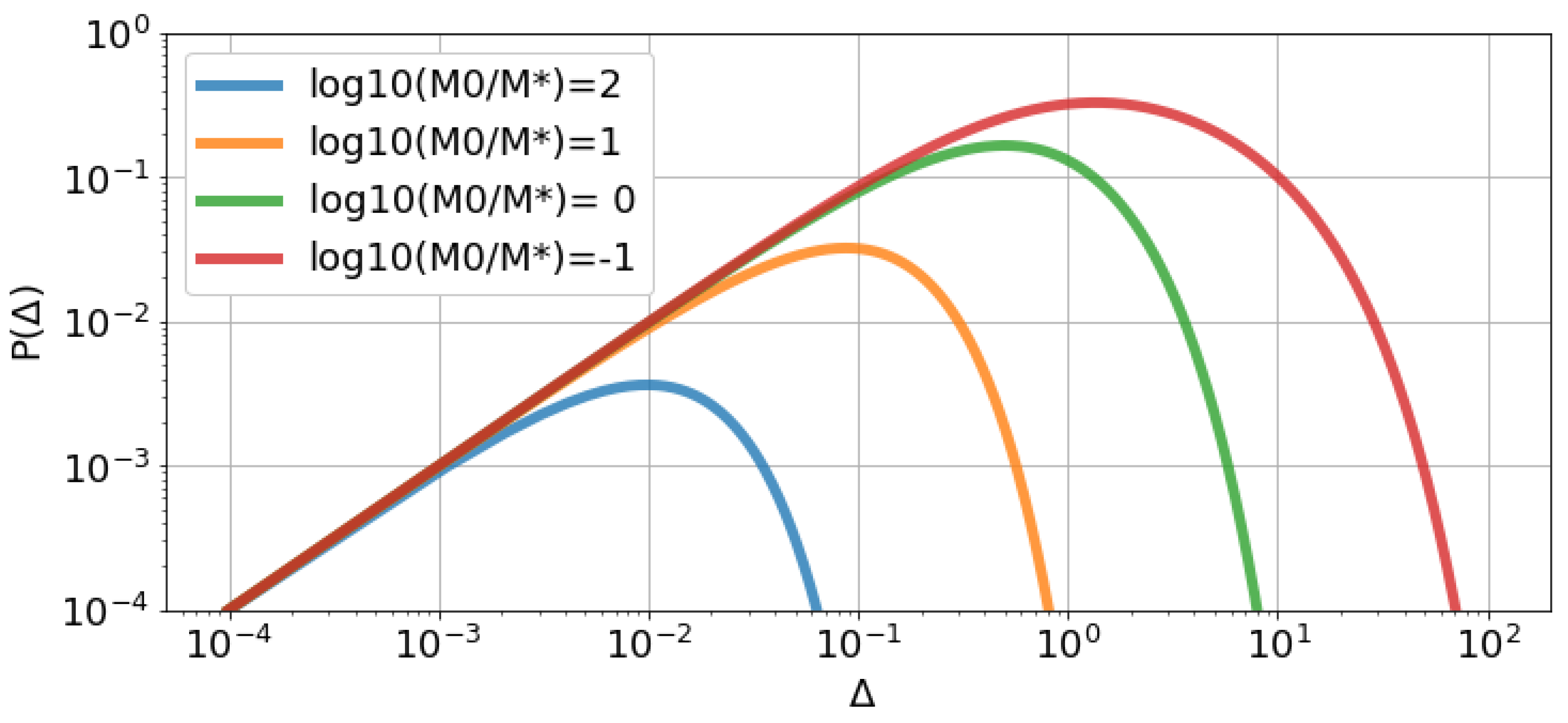
We have divided in Equation (10) by because we are interested in the relative number of BHs above the ones with the minimal mass . Figure 4 shows Equation (11) for some values of . For , the probability is dominated by the exponential suppression and peaks around . This means that most observers will live in a BH with mass . So, an accurate estimation of provides a prediction for and therefore a prediction for and , which is in agreement with the values measured in our BHU. For , the probability peaks around , which predicts that most observers live in BHs which are two times . For , the result is independent of and the peak is at . Thus, regardless of , the maximum probability corresponds to observers in a BH with mass or collapse times , which is very consistent with the measurements in our Universe for and M in Equation (3). In terms of , this corresponds to , where is the value corresponding to or .
4. Conclusions and Discussion
We propose that cosmic expansion originated from the gravitational free-fall collapse of a large and low-density matter cloud. We assume that the background is flat with and , as in empty space. The so-called flatness problem, that is solved by Inflation, is only a problem if the BB singularity can somehow create curvature. In the BHU model, the singularity is avoided at GeV (i.e., the energy corresponding to the nuclear saturation density in Equation (7)), well before Quantum Gravity effects ( GeV), so there is no reason to expect a global curvature or . There is therefore no flatness problem that needs to be solved.
In nature, we never observe cold regular matter with densities larger than that of an atomic nuclei in Equation (7). The reason for this is the Pauli exclusion principle in Quantum Mechanics, which prevents fermions from occupying the same quantum state (which includes position). This neutron degeneracy pressure is responsible for core collapse supernova explosions [18]. We propose here that when the BH collapse reaches nuclear saturation density, it bounces back, as it happens in a supernova core collapse. This Big Bounce occurs at times and energy densities that are many orders of magnitudes away from Inflation or Planck times. Thus, Quantum Gravity or Inflation are not needed to understand cosmic expansion or the monopole problem [28]. Further work is needed to understand the details of such a Big Bounce: to estimate the perturbations, composition, and the fraction of compact and diffuse remnants that resulted from the bounce. This could explain from first principles some of the free parameters in the CDM model, as shown in Table 1.
The Big Bounce could provide a uniform start for the BB, solving the horizon problem (see Figure 1 and Figure 3): super-horizon perturbations during collapse (and bounce) seed structures (BAO and galaxies) as they re-enter during expansion. The main differences with Inflation are the origin of those perturbations and the existence of a cut-off in the spectrum of fluctuations given by R in Equation (4). Such a cut-off has recently been measured in CMB maps [12,39,40,41]. Galaxy maps are also able to measure this signal [42,43]. The existence of such super-horizon perturbations could be related to the tension in measurements of the cosmological parameters from different cosmic scaletimes [44,45,46,47,48], which have similar variations in cosmological parameters to the measured CMB cut-off anomalies, as reported in [35].
Another difference is the possibility that DM is all made of primordial BHs (PBHs) and Neutron Stars (NSs) remnants from before the BB explosion. According to the PS formalism in Section 3, we expect a significant number of large (super massive) PBHs with as well as a much larger number of smaller ones. This could represent a paradigm shift for models of galaxy formation. There is a tight empirical relation between the BH mass measured in the center of large galaxies and the stellar (bulge) mass or luminosity [49]. This is hard to explain in current models of galaxy formation where galaxies form first and central BHs grow later. In the BHU model, large PBHs could instead be the seeds to form massive galaxies, which together with smaller PBHs and NSs could be the mysterious DM. This could also help explain some recent JWST observations of high redshift massive galaxies [50,51] and the puzzling observation of very luminous quasars (which trace super-massive BHs) at very high redshift (see [52] and references there in). Smaller BHs could be present as a dormant population, which could be detected with GAIA measuremnts [53].
The BH collapse time in Equation (5) is proportional to M, so that a large mass in Equation (3) is just the right one to allow enough time for galaxies and planets to form before the de-Sitter phase dominates. This provides an anthropic explanation [54,55] as to why we live inside such a large BH. In other words, it is an explanation of why the observed is so small and why we live at a time when the expansion is close to the dS phase (the coincidence problem in cosmology [1,2,7,8]). According to Equation (11) (see also Figure 4), the maximum probability corresponds to observers that appear in BHs with , where is the value corresponding to in Equation (8) for the minimum time needed for observers to exit. If we assume that this time agrees with the age of our galaxy, we find good agreement between this prediction and the observed measurements (). These arguments neglect the global rotation of the FLRW cloud (or the BHU). Such rotation could slow down the expansion rate (see Appendix C in [12]) and play some role in the bounce and collapse time. If our BHU is moving or rotating, within the Apollonian background, this could show as a dipole. A CMB dipole has already been observed [56], but it is usually interpreted as a local flow. This interpretation has recently been challenged by new observations of our local neighborhood (see [57]).
The BHU solution can also be used to understand the interior of regular (stellar or galactic) BHs. Such BHs could just be made of regular (baryonic) collapsing matter, but they will not have time to form regular galaxies or stars inside because within seconds of the bounce (see Equation (5)), the internal dynamics becomes dominated by the de-Sitter phase (caused by their event horizon mass ). The bounce proposed here, based in Quantum Mechanics, could avoid both the BH and the BB singularities [58,59], which in the BHUs model both corresponds to the same FLRW cloud collapse (but with different masses). The BHU also eludes the entropy paradox [4] in a similar way as that proposed by Penrose [5]. The difference is that the BHU does not require new laws (infinite conformal re-scaling) or cyclic repetition. Our expansion will end up trapped (and asymtotically static) inside a BH within a larger and older manifold possibly containing other BHUs. We call this the Apollonian Universe (see Section 3). Such an idea provides another layer to the Copernicus Principle, where we are not at the center of our BHU and our BHU is not at the center of everything else.
Funding
This work was partially supported by grants from Spain MCIN/AEI/10.13039/501100011033 grants PGC2018-102021-B-100, PID2021-128989NB-I00 and Unidad de Excelencia María de Maeztu CEX2020-001058-M and from European Union funding LACEGAL 734374 and EWC 776247. IEEC is funded by Generalitat de Catalunya.
Data Availability Statement
No new data is presented.
Acknowledgments
I want to thank Marco Bruni, Robert Caldwell, Benjamin Camacho, Ramin G. Daghigh, Ravi Sheth and Alberto Diez-Tejedor for their feedback to early drafts of this work and to Angela Olinto and Sergio Assad for their hospitality during the summer of 2022, when the latest version of this paper was completed, extracted from earlier unpublished drafts [60,61], which preceded later review articles [12,62].
Conflicts of Interest
The authors declare no conflict of interest.
Appendix A. Expanding Background
To form a BHU during an explosion or rapid expansion, we need a scalar field and a False Vacuum (FV), , which is a term that is explained next.
Appendix A.1. Scalar Field in Curved Space-Time
Consider a minimally coupled scalar field with:
The Lagrange equations are: . We can estimate from its definition:
to find (e.g., see [2]):
comparing with a perfect fluid in spherical coordinates:
we find:
In general, we can have for non canonical scalar fields (see Equation (5) in [63] for further details). The stable solution corresponds to :
where is trapped in the true minimum or some False Vacuum (FV) state . The situation is illustrated in Figure A1. The solution to Equation (A2) for constant (without matter or radiation) for a general metric with spherical symmetry in physical coordinates:
is given by the deSitter (dS) metric:
This metric is static, which indicates that the vacuum solution is in equilibrium. This same dS solution also corresponds to the FLRW metric solution with constant H:
If we use , so that there is empty space outside (see paper I), this corresponds to a BHU with , without regular matter or radiation. Note how the smaller the , the larger the M. Note that in general, we would not expect so that the metric outside is not that of Schwarzschild. This would correspond to a BHU inside a dS or FLRW metric (see bottom right panel of Figure A2 in paper I).
Figure A1.
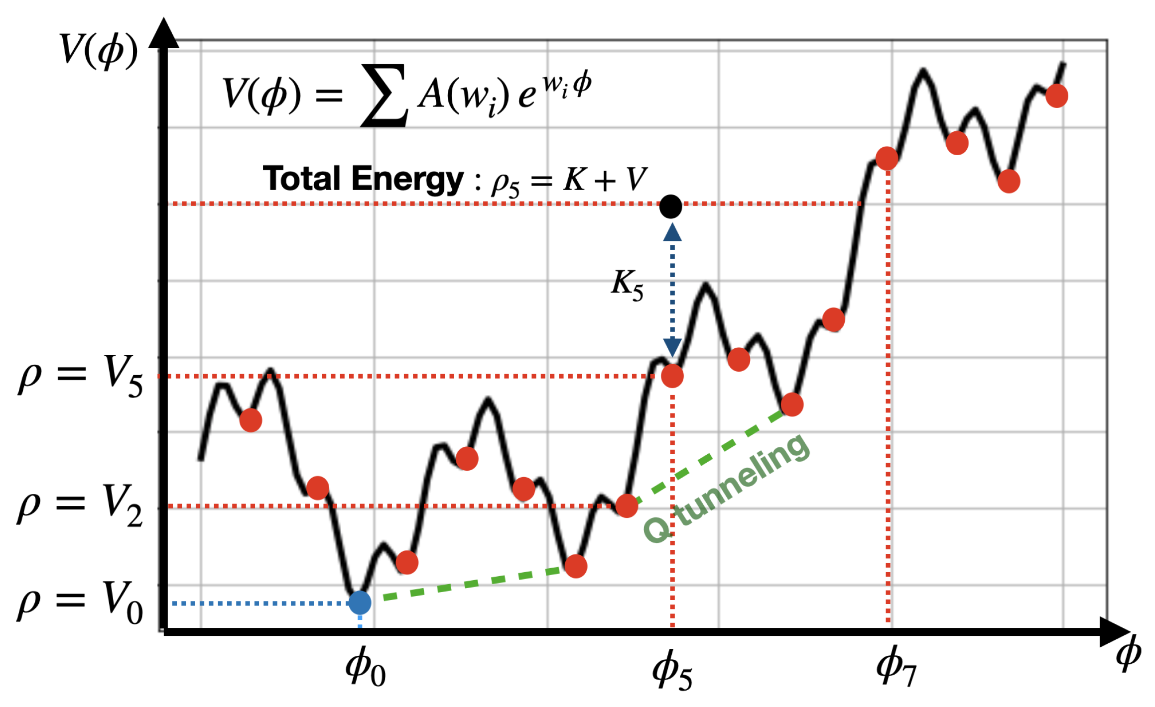
The potential , of a classical scalar field , made of the superposition of plane waves. A configuration with total energy: (black dot at ) can lose its kinetic energy during expansion (e.g., a supernova explosion or a expanding background) due to Hubble damping and relax into one of the static () ground states (or FV) (red dots). This can generate a Black Hole (BH.fv) and regular matter from reheating. Each FV has an energy excess over the true vacuum at (blue dot). Quantum tunneling (dashed lines) could allow to jump between FV, resulting in BH evaporation and new matter/radiation.
Figure A1.
The potential , of a classical scalar field , made of the superposition of plane waves. A configuration with total energy: (black dot at ) can lose its kinetic energy during expansion (e.g., a supernova explosion or a expanding background) due to Hubble damping and relax into one of the static () ground states (or FV) (red dots). This can generate a Black Hole (BH.fv) and regular matter from reheating. Each FV has an energy excess over the true vacuum at (blue dot). Quantum tunneling (dashed lines) could allow to jump between FV, resulting in BH evaporation and new matter/radiation.

Appendix A.2. BHU Formation
Consider a localized field with some fixed total energy (black dot labeled in Figure A1). In an expanding background (such as a supernovae explosion or Inflation), the field can rapidly lose its kinetic energy (), due to Hubble damping, and end up trapped inside some FV (). If the outside background () has at a lower FV, this will generate an expanding BHU until . Because an additional FV structure can exist within a given FV, the same Hubble damping can form a BHU inside a larger BHU. When K is not fully damped, the classical reheating mechanism around a FV could also be a source of matter/radiation. There is some literature on Bubble Universe formation (e.g., see [64,65] and references therein), but they typically involve quantum gravity ideas or GR extensions. As illustrated in Figure A1, there could be a landscape of nested BHU of different masses and sizes. Such BHUs are similar to primordial BHs [66]. The masses and sizes of such BHU bare no relation with the energy of the expansion (e.g., supernova explosion or inflation) or the host object which originated the expansion. This means that if this mechanism actually occurred, a BH of any mass M can emerge out of violent expansion. For example, a stellar explosion could produce a galactic size BH or one as large as our Universe. The smaller the , the larger the M and . In addition, quantum tunneling (see Figure A1) could generate a cascade of small BHs turning into larger BHs. This could take some time, as the tunneling probability is proportion to . These are puzzling results that strongly depend on the vacuum structure of , but they could explain how large mass BHUs formed.
References
- Dodelson, S. Modern Cosmology; Academic Press: New York, NY, USA, 2003. [Google Scholar]
- Weinberg, S. Cosmology; Oxford University Press: Oxford, UK, 2008. [Google Scholar]
- Tolman, R.C. On the Problem of the Entropy of the Universe as a Whole. Phys. Rev. 1931, 37, 1639–1660. [Google Scholar] [CrossRef]
- Dyson, L.; Kleban, M.; Susskind, L. Disturbing Implications of a Cosmological Constant. J. High Energy Phys. 2002, 2002, 011. [Google Scholar] [CrossRef]
- Penrose, R. Before the big bang: An outrageous new perspective and its implications for particle physics. Conf. Proc. C 2006, 060626, 2759–2767. [Google Scholar]
- Brandenberger, R. Initial conditions for inflation—A short review. Int. J. Mod. Phys. D 2017, 26, 1740002. [Google Scholar] [CrossRef]
- Peebles, P.J.; Ratra, B. The cosmological constant and dark energy. Rev. Mod. Phys. 2003, 75, 559–606. [Google Scholar] [CrossRef]
- Carroll, S.M.; Remmen, G.N. A nonlocal approach to the cosmological constant problem. Phys. Rev. D 2017, 95, 123504. [Google Scholar] [CrossRef]
- Gaztañaga, E. The Black Hole Universe, part I. Symmetry 2022, 14, 1849. [Google Scholar] [CrossRef]
- Gaztañaga, E. The size of our causal Universe. Mon. Not. R. Astron. Soc. 2020, 494, 2766–2772. [Google Scholar] [CrossRef]
- Gaztañaga, E. The cosmological constant as a zero action boundary. Mon. Not. R. Astron. Soc. 2021, 502, 436–444. [Google Scholar] [CrossRef]
- Gaztañaga, E. How the Big Bang Ends up Inside a Black Hole. Universe 2022, 8, 257. [Google Scholar] [CrossRef]
- Özel, F.; Freire, P. Masses, Radii, and the Equation of State of Neutron Stars. Annu. Rev. Astron. Astrophys. 2016, 54, 401–440. [Google Scholar] [CrossRef]
- Järvinen, M. Holographic modeling of nuclear matter and neutron stars. Eur. Phys. J. C 2022, 82, 282. [Google Scholar] [CrossRef]
- Press, W.H.; Schechter, P. Formation of Galaxies and Clusters of Galaxies by Self-Similar Gravitational Condensation. ApJ 1974, 187, 425–438. [Google Scholar] [CrossRef]
- Bernardeau, F.; Colombi, S.; Gaztañaga, E.; Scoccimarro, R. Large-scale structure of the Universe and cosmological perturbation theory. Phys. Rep. 2002, 367, 1–248. [Google Scholar] [CrossRef]
- Bertschinger, E.; Gelb, J.M. Cosmological N-body simulations. Comput. Phys. 1991, 5, 164–175. [Google Scholar] [CrossRef]
- Baym, G.; Pethick, C. Physics of neutron stars. Annu. Rev. Astron. Astrophys. 1979, 17, 415–443. [Google Scholar] [CrossRef]
- Novello, M.; Bergliaffa, S.E.P. Bouncing cosmologies. Phys. Rep. 2008, 463, 127–213. [Google Scholar] [CrossRef]
- Ijjas, A.; Steinhardt, P.J. Bouncing cosmology made simple. Class. Quantum Gravity 2018, 35, 135004. [Google Scholar] [CrossRef]
- Popławski, N. Universe in a Black Hole in Einstein-Cartan Gravity. ApJ 2016, 832, 96. [Google Scholar] [CrossRef]
- Boyle, L.; Finn, K.; Turok, N. CPT-Symmetric Universe. PRL 2018, 121, 251301. [Google Scholar] [CrossRef]
- Boyle, L.; Finn, K.; Turok, N. The Big Bang, CPT, and neutrino dark matter. Ann. Phys. 2022, 168767. [Google Scholar] [CrossRef]
- Carr, B.; Kühnel, F. Primordial Black Holes as Dark Matter: Recent Developments. Annu. Rev. Nucl. Part. Sci. 2020, 70, 355–394. [Google Scholar] [CrossRef]
- Bird etal, S. Snowmass2021 Cosmic Frontier White Paper:Primordial Black Hole Dark Matter. arXiv 2022, arXiv:2203.08967. [Google Scholar]
- Cyburt, R.H.; Fields, B.D.; Olive, K.A.; Yeh, T.H. Big bang nucleosynthesis: Present status. Rev. Mod. Phys. 2016, 88, 015004. [Google Scholar] [CrossRef]
- Starobinskiǐ, A.A. Spectrum of relict gravitational radiation and the early state of the universe. Soviet J. Exp. Theor. Phys. Lett. 1979, 30, 682. [Google Scholar]
- Guth, A.H. Inflationary universe: A possible solution to the horizon and flatness problems. Phys. Rev. D 1981, 23, 347–356. [Google Scholar] [CrossRef]
- Linde, A.D. A new inflationary universe scenario. Phys. Lett. B 1982, 108, 389–393. [Google Scholar] [CrossRef]
- Albrecht, A.; Steinhardt, P.J. Cosmology for Grand Unified Theories with Radiatively Induced Symmetry Breaking. Phys. Rev. Lett. 1982, 48, 1220–1223. [Google Scholar] [CrossRef]
- Liddle, A.R. Observational tests of inflation. arXiv 1999, arXiv:astro-ph/9910110. [Google Scholar]
- Harrison, E.R. Fluctuations at the Threshold of Classical Cosmology. Phys. Rev. D 1970, 1, 2726–2730. [Google Scholar] [CrossRef]
- Zel’Dovich, Y.B. Reprint of 1970A&A.....5...84Z. Gravitational instability: An approximate theory for large density perturbations. Astron. Astrophys. 1970, 500, 13–18. [Google Scholar]
- Peebles, P.J.E.; Yu, J.T. Primeval Adiabatic Perturbation in an Expanding Universe. ApJ 1970, 162, 815. [Google Scholar] [CrossRef]
- Gaztanaga, E.; Camacho-Quevedo, B. Super-Horizon Modes and Cosmic Expansion. arXiv 2022, arXiv:2204.10728. [Google Scholar]
- Sheth, R.K.; Tormen, G. Large-scale bias and the peak background split. Mon. Not. R. Astron. Soc. 1999, 308, 119–126. [Google Scholar] [CrossRef]
- Xiang, M.; Rix, H.W. A time-resolved picture of our Milky Way’s early formation history. Nature 2022, 603, 599–603. [Google Scholar] [CrossRef] [PubMed]
- Dalrymple, G.B. The age of the Earth in the twentieth century: A problem (mostly) solved. Geol. Soc. Lond. Spec. Publ. 2001, 190, 205–221. [Google Scholar] [CrossRef]
- Fosalba, P.; Gaztañaga, E. Explaining cosmological anisotropy: Evidence for causal horizons from CMB data. Mon. Not. R. Astron. Soc. 2021, 504, 5840–5862. [Google Scholar] [CrossRef]
- Gaztañaga, E.; Fosalba, P. A peek outside our Universe. Symmetry 2022, 14, 285. [Google Scholar] [CrossRef]
- Camacho, B.; Gaztañaga, E. A measurement of the scale of homogeneity in the Early Universe. arXiv 2021, arXiv:2106.14303. [Google Scholar]
- Gaztanaga, E.; Baugh, C.M. Testing deprojection algorithms on mock angular catalogues: Evidence for a break in the power spectrum. Mon. Not. R. Astron. Soc. 1998, 294, 229–244. [Google Scholar] [CrossRef][Green Version]
- Barriga, J.; Gaztañaga, E.; Santos, M.G.; Sarkar, S. On the APM power spectrum and the CMB anisotropy: Evidence for a phase transition during inflation? Mon. Not. R. Astron. Soc. 2001, 324, 977–987. [Google Scholar] [CrossRef]
- Colin, J.; Mohayaee, R.; Rameez, M.; Sarkar, S. Evidence for anisotropy of cosmic acceleration. Astron. Astrophys. 2019, 631, L13. [Google Scholar] [CrossRef]
- Riess, A.G. The expansion of the Universe is faster than expected. Nat. Rev. Phys. 2019, 2, 10–12. [Google Scholar] [CrossRef]
- Di Valentino, E.; Mena, O.; Pan, S.; Visinelli, L.; Yang, W.; Melchiorri, A.; Mota, D.F.; Riess, A.G.; Silk, J. In the realm of the Hubble tension-a review of solutions. Class. Quantum Gravity 2021, 38, 153001. [Google Scholar] [CrossRef]
- Abdalla, E.; Abellán, G.F.; Aboubrahim, A.; Agnello, A.; Akarsu, Ö.; Akrami, Y.; Alestas, G.; Aloni, D.; Amendola, L.; Anchordoqui, L.A.; et al. Cosmology Intertwined: A Review of the Particle Physics, Astrophysics, and Cosmology Associated with the Cosmological Tensions and Anomalies. arXiv 2022, arXiv:2203.06142. [Google Scholar] [CrossRef]
- Castelvecchi, D. How fast is the Universe expanding? Cosmologists just got more confused. Nature 2019, 571, 458–459. [Google Scholar] [CrossRef]
- Gültekin, K.; Richstone, D.O.; Gebhardt, K.; Lauer, T.R.; Tremaine, S.; Aller, M.C.; Bender, R.; Dressler, A.; Faber, S.M.; Filippenko, A.V.; et al. The M-σ and M-L Relations in Galactic Bulges, and Determinations of Their Intrinsic Scatter. ApJ 2009, 698, 198–221. [Google Scholar] [CrossRef]
- Liu, B.; Bromm, V. Accelerating early galaxy formation with primordial black holes. arXiv 2022, arXiv:2208.13178. [Google Scholar]
- Menci, N.; Castellano, M.; Santini, P.; Merlin, E.; Fontana, A.; Shankar, F. High-Redshift Galaxies from Early JWST Observations: Constraints on Dark Energy Models. arXiv 2022, arXiv:2208.11471. [Google Scholar]
- Ma, L.; Hopkins, P.F.; Ma, X.; Anglés-Alcázar, D.; Faucher-Giguère, C.A.; Kelley, L.Z. Seeds don’t sink: Even massive black hole ’seeds’ cannot migrate to galaxy centres efficiently. Mon. Not. R. Astron. Soc. 2021, 508, 1973–1985. [Google Scholar] [CrossRef]
- El-Badry, K.; Rix, H.W.; Quataert, E.; Howard, A.W.; Isaacson, H.; Fuller, J.; Hawkins, K.; Breivik, K.; Wong, K.W.K.; Rodriguez, A.C.; et al. A Sun-like star orbiting a black hole, 2022. arXiv 2022, arXiv:2209.06833. [Google Scholar]
- Tegmark, M.; Rees, M.J. Why Is the Cosmic Microwave Background Fluctuation Level 10−5? Astrophys. J. 1998, 499, 526–532. [Google Scholar] [CrossRef][Green Version]
- Garriga, J.; Vilenkin, A. Testable anthropic predictions for dark energy. Phys. Rev. D 2003, 67, 043503. [Google Scholar] [CrossRef]
- Smoot, G.F.; Bennett, C.L.; Kogut, A.; Wright, E.L.; Aymon, J.; Boggess, N.W. Structure in the COBE Differential Microwave Radiometer First-Year Maps. Astrophys. J. 1992, 396, L1. [Google Scholar] [CrossRef]
- Secrest, N.J.; von Hausegger, S.; Rameez, M.; Mohayaee, R.; Sarkar, S.; Colin, J. A Test of the Cosmological Principle with Quasars. Astrophys. J. 2021, 908, L51. [Google Scholar] [CrossRef]
- Penrose, R. Gravitational Collapse and Space-Time Singularities. Phys. Rev. Lett. 1965, 14, 57–59. [Google Scholar] [CrossRef]
- Dadhich, N. Singularity: Raychaudhuri equation once again. Pramana 2007, 69, 23. [Google Scholar] [CrossRef][Green Version]
- Gaztañaga, E. Inside a Black Hole: The Illusion of a Big Bang. 2020. Available online: https://hal.archives-ouvertes.fr/hal-03106344 (accessed on 11 January 2021).
- Gaztañaga, E. The Black Hole Universe (BHU) from a FLRW Cloud. 2021. Available online: https://hal.archives-ouvertes.fr/hal-03344159 (accessed on 14 September 2021).
- Gaztañaga, E. The Cosmological Constant as Event Horizon. Symmetry 2022, 14, 300. [Google Scholar] [CrossRef]
- Diez-Tejedor, A.; Feinstein, A. Homogeneous scalar field the wet dark sides of the universe. Phys. Rev. D 2006, 74, 023530. [Google Scholar] [CrossRef]
- Garriga, J.; Vilenkin, A.; Zhang, J. Black holes and the multiverse. J. Cosmol. Astropart. Phys. 2016, 2016, 064. [Google Scholar] [CrossRef]
- Oshita, N.; Yokoyama, J. Creation of an inflationary universe out of a black hole. Phys. Lett. B 2018, 785, 197–200. [Google Scholar] [CrossRef]
- Kusenko, A. Exploring Primordial Black Holes from the Multiverse with Optical Telescopes. Phys. Rev. Lett. 2020, 125, 181304. [Google Scholar] [CrossRef] [PubMed]
Figure 1.
The FLRW metric can be used to model: (LEFT) a CDM infinite universe with GM, where M is the (or DE) mass inside , (MIDDLE) a stellar cloud with finite mass M inside R (red circle), or (RIGHT) a BHU where R is inside (black circle). In the BHU, outside R, while in CDM, is the same everywhere. The Hubble Horizon (blue circle) is expanding (top panels) or collapsing (bottom). Matter inside (outside) is colored in cyan (yellow). In our Universe, we have . The causal perturbations of size D becomes a super-horizon () during collapse and re-enters the Hubble Horizon () during expansion, solving the horizon problem without Inflation.

Figure 2.
Hierarchical structure of BHs and halos (represented by circles) inside other BHs and halos. The smallest BHs form first. Then, larger-scale fluctuations collapse, including smaller BHs inside. The left panel shows a picture of the structure when the largest BH collapsed (outer circle). The right panel shows a merger tree which corresponds to the time evolution from top (early) to bottom (late) of the collapse of some of the small BHs as they merge into bigger ones. The last instant (the trunk of the tree) reflects the time when the largest BH has collapsed.

Figure 3.
Illustration of the formation of a BHU. Color regions (dashed red line) are filled with a uniform FLRW metric (blue corresponds to and yellow corresponds to ) with empty space outside. A cloud of radius R and mass M collapses under gravity. When it reaches , it becomes a BH. The collapse proceeds inside the BH (where a frozen layer appears in yellow) until it bounces, producing an expansion (the hot Big Bang). The event horizon behaves like a cosmological constant with so that the expansion freezes before it reaches back to . The bottom panels shows the evolution of R and during collapse and expansion in log units of . The structure in-between R and is frozen and seeds structure formation in our Universe, which could include smaller BHUs, CMB, stars and galaxies, and it replaces the role of Inflation in CDM.

Figure 4.
Anthropic probability in Equation (11) for different values of . This corresponds to the probability for an observer like us to be in a BH of mass . corresponds to the minimum time Gyr needed for a galaxy and planet similar to ours to form. is the non-linear mass scale. Regardless of , the maximum in is always within or .


Table 1.
Model comparison. Observations that require explanation.
| Cosmic Observation | Big Bang (CDM) | BHU Big Bounce |
|---|---|---|
| Expansion law | FLRW metric | FLRW metric |
| Element abundance | Nucleosynthesis | Nucleosynthesis |
| Baryons per foton | Free parameter of reheating | Diffuse remnants of collapse |
| CMB K | Recombination | Recombination |
| All sky uniformity & LSS seeds | Inflation | Big Bounce |
| Intrinsic CMB dipole | Local flow | BHU frame |
| Cosmic acceleration | Dark Energy | BH event horizon size |
| Age of the Universe: 14 Gyr | Dark Energy | BH event horizon size |
| Rot. curves, grav. lensing & vel. flows | Dark Matter | Compact remnants from collapse |
| CMB fluctuations | Inflation: free parameter | Perturbations during collapse/bounce |
| CMB sprectral index | Inflation: | Perturbations during collapse/bounce |
| Free parameter | Compact to diffuse renmants | |
| Free parameter | Time to de-Sitter phase | |
| Large-scale CMB anomalies | Cosmic Variance (bad luck) | Super-horizon cut-off |
| Hubble tension | Systematic effects | Super-horizon perturbations |
| Flat universe | Inflation | Topology of empty space |
Publisher’s Note: MDPI stays neutral with regard to jurisdictional claims in published maps and institutional affiliations. |
© 2022 by the author. Licensee MDPI, Basel, Switzerland. This article is an open access article distributed under the terms and conditions of the Creative Commons Attribution (CC BY) license (https://creativecommons.org/licenses/by/4.0/).
Share and Cite
MDPI and ACS Style
Gaztanaga, E. The Black Hole Universe, Part II. Symmetry 2022, 14, 1984. https://doi.org/10.3390/sym14101984
AMA Style
Gaztanaga E. The Black Hole Universe, Part II. Symmetry. 2022; 14(10):1984. https://doi.org/10.3390/sym14101984
Chicago/Turabian StyleGaztanaga, Enrique. 2022. "The Black Hole Universe, Part II" Symmetry 14, no. 10: 1984. https://doi.org/10.3390/sym14101984
APA StyleGaztanaga, E. (2022). The Black Hole Universe, Part II. Symmetry, 14(10), 1984. https://doi.org/10.3390/sym14101984
Note that from the first issue of 2016, this journal uses article numbers instead of page numbers. See further details here.