Article

Machine Learning-Based Hyperspectral and RGB Discrimination of Three Polyphagous Fungi Species Grown on Culture Media

by
Jan Piekarczyk
1,*,
Andrzej Wójtowicz
2,
Marek Wójtowicz
3,
Jarosław Jasiewicz
1,
Katarzyna Sadowska
2,
Natalia Łukaszewska-Skrzypniak
2,
Ilona Świerczyńska
2 and
Katarzyna Pieczul
2
1
Faculty of Geographic and Geological Sciences, Adam Mickiewicz University, 60-680 Poznań, Poland
2
Institute of Plant Protection—National Research Institute, 60-318 Poznań, Poland
3
Plant Breeding and Acclimatization Institute—National Research Institute, 60-479 Poznań, Poland
*
Author to whom correspondence should be addressed.
Agronomy 2022, 12(8), 1965; https://doi.org/10.3390/agronomy12081965
Submission received: 25 July 2022 / Revised: 16 August 2022 / Accepted: 17 August 2022 / Published: 20 August 2022
(This article belongs to the Section Pest and Disease Management)

Abstract

:
In this study, three fungi species (Botrytis cinerea, Rhizoctonia solani, Sclerotinia sclerotiorum) were discriminated using hyperspectral and red-green-blue (RGB) data and machine learning methods. The fungi were incubated at 25 °C for 10 days on potato dextrose agar in Petri dishes. The Hyperspectral data were acquired using an ASD spectroradiometer, which measures reflectance with 3 and 10 nm bandwidths over the range 350–1000 nm and the range 1000–2500 nm, respectively. The RGB images were collected using a digital Canon 450D camera equipped with the DIGIC 3 processor. The research showed the possibility of distinguishing the analysed fungi species based on hyperspectral curves and RGB images and assessing this differentiation using machine learning statistical methods (extreme boosting machine with bootstrap simulation). The best results in analysed fungi discrimination based on hyperspectral data were achieved using the Principal Component Analysis method, in which the average values of recognition and accuracy for all three species were 0.96 and 0.93, respectively. The wavelengths of the shortwave infrared (SWIR) wavelength region appeared to be the most effective in distinguishing B. cinerea-R. solani and B. cinerea-S. sclerotiorum, while of the visible range (VIS) of electromagnetic spectrum in discrimination of R. solani-S. sclerotiorum. The hyperspectral reflectance data were strongly correlated with the intensity of the pixels in the visible range (R2 = 0.894–0.984). The RGB images proved to be successfully used primarily for the identification of R. solani (recognition = 0.90, accuracy = 0.79) and S. sclerotiorum (recognition = 0.84, accuracy = 0.76). The greatest differences in the intensity of the pixels between B. cinerea and R. solani as well as R. solani and S. sclerotiorum occurred in the blue band and in distinguishing B. cinerea and S. sclerotiorum in the red band.

1. Introduction

Rapid and accurate identification of plant pathogens is essential to adopt the most appropriate plant protection strategies [1]. Two groups of methods for pathogen identification can be distinguished: direct and indirect. The direct group includes polymerase chain reaction (PCR) [2], real-time PCR [3], loop-mediated isothermal amplification (LAMP) [4], immunofluorescence (IF) [5], fluorescence in-situ hybridisation (FISH) [6], enzyme-linked immunosorbent assay (ELISA) [7], flow cytometry (FCM) [8], and gas chromatography-mass spectrometry (GC-MS) [9]. These methods proved to be highly sensitive and specific in the detection of numerous plant pathogens. However, they are not suitable for in-field analysis. In contrast with direct methods, the indirect can fulfil this task. The indirect methods include thermography and reflectance spectroscopy, among which hyperspectral, multispectral and RGB images play a significant role [10,11,12].
Over the years, the rapid development of new technologies based on hyperspectral techniques and RGB imaging has encouraged extensive research on pathogen identification [13,14,15,16,17,18]. Hyperspectral techniques provide helpful information about the analysed object based on a spectrum between 350 and 2500 nm. This method showed high sensitivity to the subtle plant changes caused by diseases, and made it possible to distinguish different disease types and perform early asymptomatic detection [19]. The RGB image is represented by three colour component intensities such as red, green, and blue, and uses 8-bit monochrome standard and has 24 bits/pixel where eight bits for each colour (red, green, and blue) [20]. The utilisation of images to evaluate diseases of plants has been practised for over three decades [21,22]. Most of the available solutions use RGB imagery to quantify symptomatic areas in the whole plant or its parts [23,24,25,26,27,28]. Recently, digital images providing appropriate colour data for this task have increased dramatically due to the availability of inexpensive instruments such as digital cameras, phones, or scanners [29]. While reflectance spectroscopy provides a massive amount of data, the next step provides novel tools to extract knowledge from such data. Machine learning has emerged among such tools, directing research to a new paradigm of data-driven science [30] and gaining popularity in various fields of agriculture such as plant breeding [31], in vitro culture [32], stress phenotyping [33], plant system biology [34], plant identification [35], and pathogen identification [36].
Numerous plant diseases are caused by Ascomycota, represented among others by Botrytis cinerea, Rhizoctonia solani and Sclerotinia sclerotiorum. These pathogens are characterised by worldwide distribution and a wide host range. Considerable threat to the agricultural production caused by B. cinerea, R. solani and S. sclerotiorum and limitation of the disease identification methods used so far triggered the incorporation of remote sensing technics into discrimination of these pathogens. The spectral pattern of B. cinerea was investigated by Aboelghar et al. [37], who tested six spectra zones for distinguishing the pathogen isolates collected from grape and strawberry and obtained the best results with the use of the short-wave infrared wavelengths. Aboelghar et al. [38] also showed the suitability of the Euclidean distance (ED) method for discrimination of that pathogen isolates. The example illustrating the use of remote sensing for R. solani discrimination is the study of Reynolds et al. [39], who focused on identifying wideband and narrowband vegetation indices optimal for the correlation of Rhizoctonia crown and root rot of sugarbeet symptoms with visual ratings of the disease. In turn, the survey conducted by Cao et al. [40] represents the study concentrated on remote sensing for S. sclerotiorum detection. The authors investigated the potential of infrared thermography to distinguish the infected and non-infected areas of the attacked oilseed rape leaves by S. sclerotiorum. They proved the possibility of improving the classification results by image fusion based on multi-model images.
The capabilities of various remote sensing techniques documented above induce new research to compare the previously proposed methods and to develop new solutions that ensure greater efficiency or lower the costs of pathogen identification. The study aimed to compare the effectiveness of three fungi species (B. cinerea, R. solani, S. sclerotiorum) discrimination based on hyperspectral measurements and RGB images using machine learning statistical methods. Additionally, we wanted to determine the most informative wavelengths and check relations between spectral reflectance data obtained using two different sensors.

2. Materials and Methods

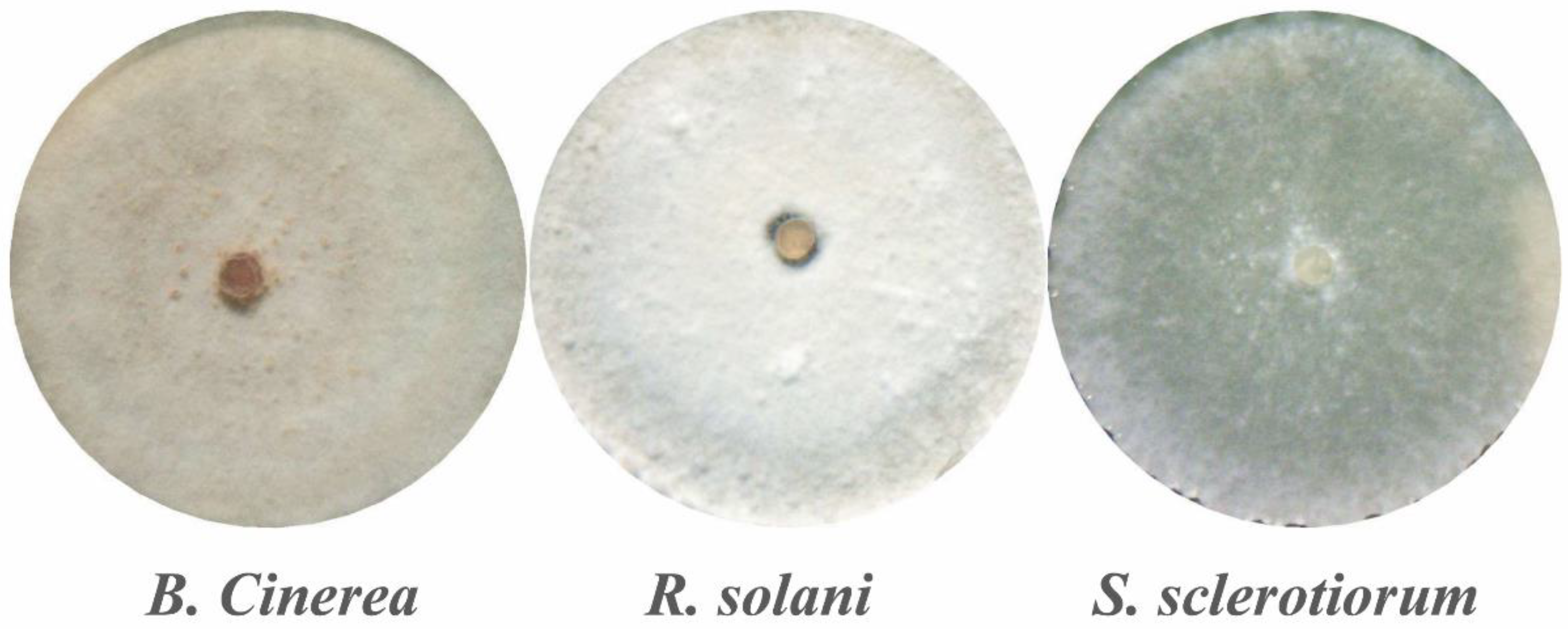
2.1. Fungal Cultures

The pathogens were isolated from rape plants with symptoms of fungal infection and deposited in Plant Disease Clinic and Bank of Pathogens, the Department of Institute of Plant Protection, National Research Institute, Poznań, Poland. The provided pathogens were maintained at 16 °C under mineral oil. The cultures were grown on PDA (Potato Dextrose Agar, Difco) medium and subcultured twice. Petri dishes were inoculated with 7-old days fungal colony plugs in the centre. Before spectral measurements, the fungi cultures were incubated at 25 °C for 10 days in the darkness (Figure 1).

2.2. Hyperspectral Measurements

The hyperspectral data were acquired using an ASD spectroradiometer (FieldSpec Analytical Spectral Devices, Inc., Boulder, CO, USA), which measures reflectance with 3 and 10 nm bandwidths over the range 350–1000 nm and the range 1000–2500 nm, respectively. Reflectance spectra were obtained as the ratio between the spectrum of a calibration panel (Spectralon: SRT-99100 UV–VIS-NIR Diffuse Reflectance Target, LabSphere Inc. North Sutton, NH 03260 USA) and that of analysed fungus cultures. All measurements were performed using a pistol grip with a 10° Field of View (FOV) and afore optics lens attached to the pistol grip at the height of 40 cm above the Petri dish illuminated by a 400 W halogen lamp positioned 90 cm from the sample at an angle of 45° to the zenith. In order to decrease the reflectance of semitransparent PDA, a black diffusing plate was placed under the Petri dish holder. Before collecting reflectance data, the spectrophotometer was warmed up for an hour and the lamp was turned on appropriately earlier so that the temperature was saturated, and the output light was stable. The reflectance from each fungi culture in a Petri dish was measured four times at four different dish positions. For each fungal species, 40 measurements were made in total.

2.3. RGB Images

Digital Canon 450D camera equipped with the DIGIC 3 processor was used to collect the RGB images in JPG (Joint Photographic Experts Group) format. It is a 12.0 megapixels digital single-lens reflex camera (DSLR) with a maximum resolution of 4272 × 2848. To calculate mean DN (digital number) values from RGB images of each Petri dish, the MIPS TNT™ software (Microimages Inc. Lincoln NE, USA) was used. The DN of the pixel express the intensity of the radiation reflected or emitted from the part of the surface represented by that pixel in the image. The band maxima for R, G, and B wavelengths for the Canon EOS 450D were calculated by Cameron and Kumar [41] and were 600, 540 and 450 nm, respectively.

2.4. Data Processing and Models Created

Spectral measurements provided 808 spectral curves. Each curve has 2151 individual bands, which means 2151 potential predictors. From a data science point of view, the collected data set is not large, smaller than the number of estimators. Such a situation is not unusual in natural science projects, where many factors, primarily the possibility of obtaining a sufficiently large number of unique samples, limits the number of cases. The entire procedure is outlined in Figure 2 and consists of three stages: (1) preprocessing, (2) feature selection and (3) learning.

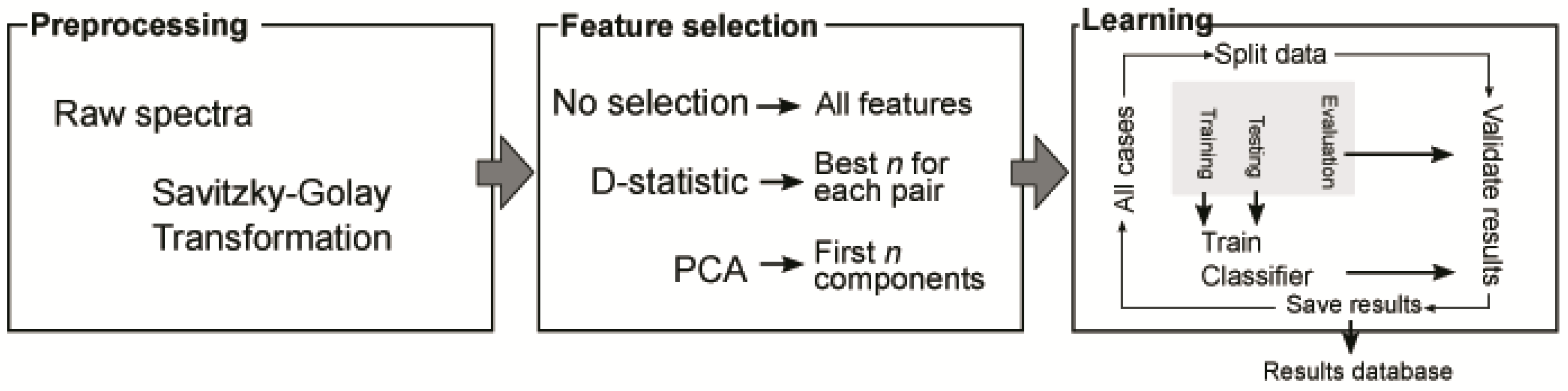
2.4.1. Preprocessing and Feature Selection

Raw spectra require transformation before further processing. Based on our previous experiences [42], we selected a Savitzky–Golay (SG) filter [43]. The SG filter uses local derivatives and therefore is more robust against spectra imperfections than simple methods such as basement alignment or continuum removal. The SG filter removes unnecessary effects resulting from the non-ideal sampling process, like noise reduction or baseline shift. SG filter requires three parameters: differentiation order, polynomial order, and size of the smoothing window. By experiments, we found that the following values, respectively: 2, 2 and 5 provide locally optimal results. Wavelengths values after SG transformation became input features for target classifiers. The target classifier is an Extreme gradient boosting classifier-XGBoost [44]. XGBoost has been designed to process non-linear data and allows extracting important features from datasets containing noise and redundant information. Numerous studies [45,46,47] demonstrate the highest prediction accuracy and provides remarkable results for spectral analyses in different scientific domains. Using all predictors, especially with many features, results in a very long training time. For that reason, in the second step, besides using all 2151 features, we independently applied two additional feature selection methods due to the significant advantage of quantity in the number of features over the cases. As the first, we limited the number of features to the restricted group of most divisive bands, and in the second, we used standard Principal Component Analysis (PCA). In that way, in the paper, we test three scenarios of feature selection: (1) all features, (2) most divisive bands, and (3) PCA.
The first scenario does not require any additional steps. In the second scenario, we selected a group of spectrum bands most important for the distinction of species. As “the most important”, we define those bands whose distributions overlap to the slightest degree for the studied populations. We used the value of two-sample Kolmogorov-Smirnov (K-S) D-statistic as a variable importance index [48]. D-statistics takes values between 0 and 1 where 0 means full overlap and 1 means full separation, which means that the higher the value, the higher separation. The D-statistic does not require an assumption on the form of the distributions of compared sets. For each wavelength, D-statistic was calculated using:
D = sup x | F ( x ) G ( x ) |
where F(x) and G(x) are two cumulative distribution functions, and supx is the supremum of those two distributions. This means that the D takes the largest absolute difference between F(x) and G(x) across all x values.
The D statistic was calculated for all possible combinations of variables, in our case-three: B cinerea-R. solani, B. cinerea-S. sclerotiorum, R. solani-S. sclerotiorum. We used the analysis of each pair because the features separating one pair may not be relevant to the others. By increasing the number of the best predictors for each pair, we have observed that beyond eight, the accuracy of the model does not increase. Next, we applied a cross product on all three subsets to eliminate duplicates. Thus, we found a minimal set of 10 variables that allow us to achieve the highest accuracy of the classifier. The second scenario involves the standard PCA on the transformed and z-scored data. In a similar way as in the former scenario, we found that beyond eight principal components, the accuracy of the model remains constant.

2.4.2. Learning Process

The typical procedure of training the XGBoost classifier requires dividing the collected data into three sets [49,50]. Two sets, the training and the testing set, are used during the training of the model, where the testing set allows us to report how well the model is performing on the given stage of the training and, in effect, to avoid over-fitting. The third is the evaluation set, which is used for independent validation of the model accuracy. With a relatively small number of cases compared to the number of features, the role of features in the trained model may vary significantly for the various components of the training, testing, and evaluation sets. The consequence of such a situation is the model’s potential over-fitting [51]. Machine learning models gain their highest performance when the distributions of selected features in all subsets are very similar. This is not the case when the number of cases surpasses the number of features, but when the data set is relatively small, there is a risk that predictors selected in the training subset will not be relevant to those left for evaluation. Such a situation results mainly in the high efficiency of the training set and low efficiency during evaluation. Also, in small data sets, even a minor number of potentially “bad” cases (for example, corrupted, contaminated or incorrectly measured) have a substantial impact on the entire classifier and may lead to wrong conclusions about the entire analytical procedure. In the first step, we set up a classifier using softmax as a learning task and logloss as an evaluation metric. Other hyperparameters we tuned individually for each scenario and input data. We applied a bootstrapping procedure, including 200 iterations, to determine the risk of over-fitting and identify potentially problematic cases in our data. If an over-fitting risk is high in such a data set, we expect the testing set’s performance to vary between iterations. If such a risk is low, each iteration shall return with similar, possibly high performance. Moreover, if there are strong predictors in the data, the trained model will select them at each iteration, and each iteration will indicate the same cases each time.
All 808 cases were randomly divided into the training set at each iteration, including 60% of cases, testing sets, including 20% of cases, and the evaluation set with the remaining 20%. This means that we have 200 variant training sets assessed by 200 different testing sets, and each case had a chance to be included in the testing set 40 times on average. It is a large enough number to assess the stability of the classification process. At each iteration, we save the results of the evaluation and finally, each case is described by the number of correct and incorrect hits. To assess each case individually [52], we propose that each case is determined in three ways: (1) correctly classified (Good case) if the outcome agrees with the actual in more than 85% hits; (2) incorrectly classified (Wrong case) if the outcome shows a different label than the actual, but steady, namely, more than 85% hits for a wrong case; (3) Vague case if the outcome takes different labels at each iteration—the threshold 85% was selected arbitrarily. The second indicates that the case is more similar to another species than its parent in the measured wavelengths. The third situation indicates that the classifier cannot be trained efficiently for the given case. Bootstrap does not allow traditional performance measures like sensitivity or specificity. For this reason, to evaluate the performance, we use the classically defined accuracy (Acc) as the ratio of correctly classified objects to the total number of classified objects in this class and recognition (Rec), an average percentage of correct hits for the individual. The two measures are non-standard and apply only to bootstrapping evaluations; however, Acc has the same meaning as accuracy in multiclass classification, namely the fraction of correct classification.
ACC = G/(G + V + W)
where: G-number of good; V-number of vague; W-number of wrong
REC = avg (hc/h)
where: hc-correct hits; h-total hits.

3. Results and Discussion

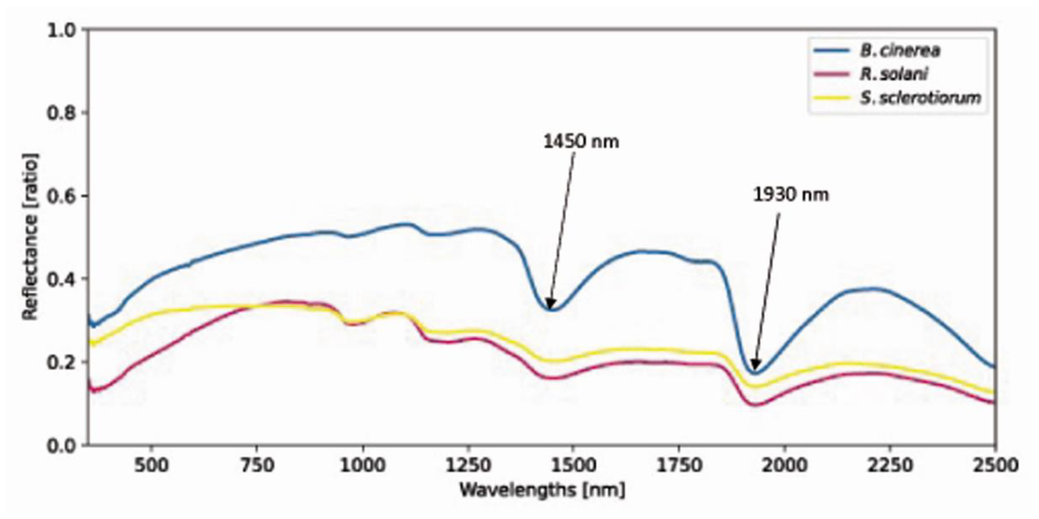
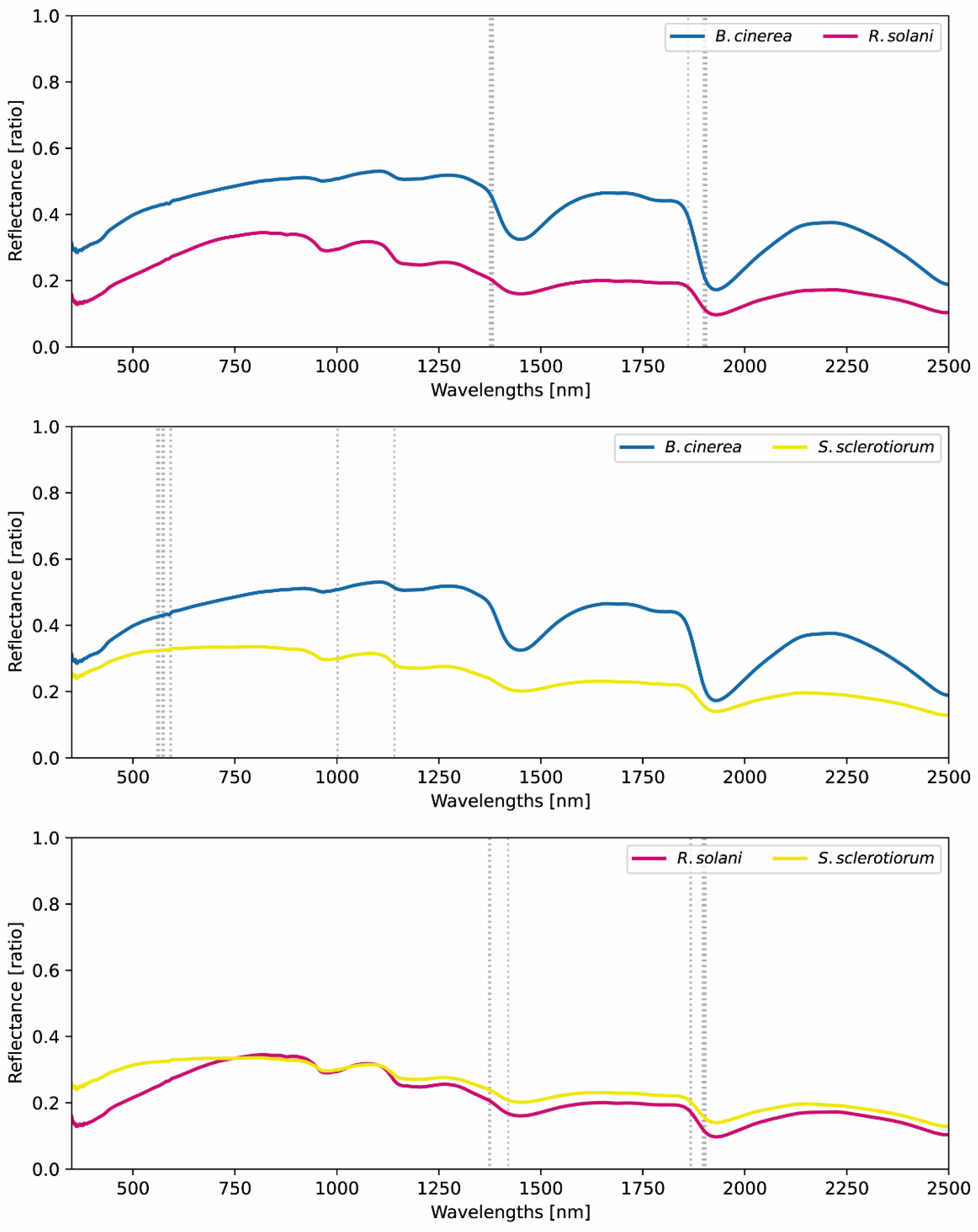
3.1. Hyperspectral Characteristics of Fungi

Hyperspectral measurements are performed using spectrophotometers that record the reflected radiation in very many (more than 100) very narrow bands of wavelengths. The reflectance characteristics of an object over different, contiguous wavelengths are graphically represented by reflectance curves (spectra).
As shown in Figure 3, the spectra of B. cinerea, R. solani and S. sclerotiorum differed visibly in the visible range (VIS) of the electromagnetic spectrum. In the whole range, the spectrum of B. cinerea stood out from the others, and was characterised by the highest reflectance and the most clearly marked water absorption bands with the maximum at 1450 nm and 1930 nm. The spectral characteristic of B. cinerea is very similar to those presented in the work of Aboelghar et al. [37], who used spectral measurements to distinguish isolates of this pathogen. The differences in the course of the spectra were noted only in the range of about 700 nm. The spectral curve presented by Aboelghar et al. [38] was characterised by an increase in reflectance in this range; however, this was not observed in our research.
The comparison of the spectral characteristics of the three species is presented in Figure 4. The highest differences in the whole optical range appeared between the spectra of B. cinerea and R. solani. Similar differences were observed between B. cinerea and S. sclerotiorum spectra, except for the VIS range and the second water absorption band in SWIR wavelength region. On the other hand, the minor differences were registered between R. solani and S. sclerotiorum. In this case, the highest differences were observed in the VIS spectrum. In the visible range, the reflectance of B. cinerea and R. solani showed a marked increase with increasing wavelength, while the reflectance of S. sclerotiorum was only recorded in the blue range.
The most valuable wavelengths for discrimination of B. cinerea and R. solani and B. cinerea and S. sclerotiorum were found in the SWIR range, on the descending portion of the water absorption bands close to their maxima, which occur in 1450 and 1950 nm. The usefulness of SWIR in distinguishing fungi grown on fungal culture media was also noted by Aboelghar et al. [37], who based on the results of research on distinguishing between B. cinerea, Aspergillus sp., Rhizopus sp., Penicillium italicum, Penicillium digitatum, Fusarium sp., Alternaria sp. Rhizoctonia sp. found the 2055–2315 nm wavelength range to be the most useful. However, in these studies, they did not consider the ranges covering the water absorption bands because the measurements were made outdoors. The advantages of SWIR in the study of B. cinerea were also demonstrated by Conrad et al. [53], who, comparing the spectral characteristics of inoculated and healthy rice plants in the range of 1898–2551 nm, found differences in the intensity of reflectance in the range of 1564–1854 nm.
In studies on remote sensing to distinguish B. cinerea from F. oxysporum, Aboelghar et al. [38] demonstrated the usefulness of wavelengths in the visible and near-infrared (VNIR) range (350–1300 nm). In our study, VNIR also proved to be the most useful for distinguishing R. solani and S. sclerotiorum. The best wavelengths for differentiation between these two species were mostly in the VIS range (wavelengths 563–593 nm) and shorter wavelengths in near-infrared (NIR) range (Figure 4 and Table 1). Another example illustrating the usefulness of spectral measurements in the VNIR range for pathogen recognition are the studies by Kong et al. [54], who, identifying S. sclerotiorum on rapeseed stems based on spectral characteristics in the 384–1034 range, included the VIS wavelengths among the most valuable wavelengths. Including these in our research turned out to be optimal.
The applied classification methods showed very high accuracy, exceeding 85%. The highest number of correctly classified cases of B. cinerea (163) and S sclerotiorum (269) was obtained using the PCA method (Table 2). On the other hand, the all-features method generated the most correctly classified R. solani cases (270). Similar results were obtained with the use of the Rec and Acc indices. The most significant number of cases of good diagnosis and the highest mean values of the Rec and Acc indicators for all three species were obtained due to the application of the PCA method. This method turned out to be the most accurate in the classification of S. sclerotiorum (95%) and the worst in the classification of B. cinerea (91%). The accuracy of the Selected Features method did not exceed 90% for any of the fungi analysed.

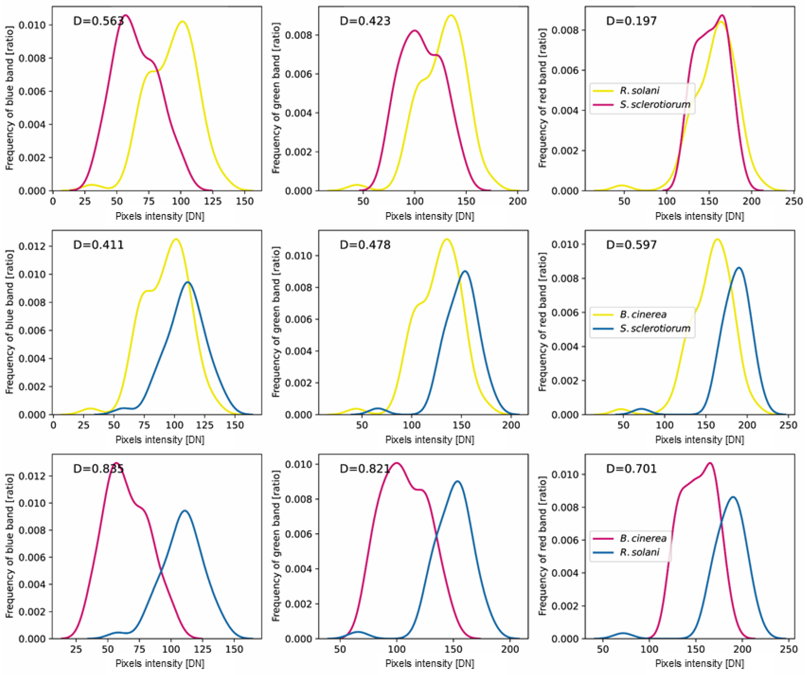
3.2. RGB Characteristics of Fungi

An RGB (truecolor) image consists of individual pixels for which red, green, and blue components are defined. The light intensity level of each of these three components is encoded as Digital Number (DN) in the range from 0 to 255. Thus, each pixel colour of an RGB image is a mixture of light from the three bands, and DN on the red, green, and blue channels can be extracted from this image.
The D-statistics presented in Figure 5 show that the most remarkable differences in the mean pixel intensity values from RGB images occurred between B. cinerea and R. solani. The most significant differences were recorded in the blue band (D = 0.84) and the smallest in the red band (D = 0.70). The most minor difference in mean pixel intensity values was when comparing R. solani and S. sclerotiorum. In this case, the differences were also the largest in the blue band (D = 0.56) and the smallest in the red band (D = 0.20). On the other hand, the opposite situation was observed when comparing B. cinerea and S. sclerotiorum. The D-statistics in the blue, green and red bands were 0.41, 0.48, and 0.60, respectively.
The helpfulness of digital imaging in the discrimination of disease symptoms is well documented in many studies [55,56,57,58,59]. The advantages of the blue band in terms of pathogen identification were presented by Fernández et al. [60], who distinguished healthy and Podosphaera xanthii (powdery mildew)-infested cucumber leaves with an accuracy of 0.89% based on the multispectral RGB (mRGB) image (R = 663–673, G = 550–570, B = 465–485 nm) and images from the blue channel. Another example illustrating an application of RGB images in fungi discrimination is delivered by Pozza et al. [61], who analysed the infestation of common beans seeds by Aspergillus flavus, A. niger, A. ochraceus, Penicillium sp., Mucor sp, Rhizopus sp, Fusarium sp, Rhizoctonia sp. His study showed that, among the six algorithms used (random forest (rf), rpart, rpart1SE, rpart2, naive Bayes, and svmLinear2), the best results were guaranteed by Random Forest ensuring the classification accuracy of 0.80 Kappa 0.77. In a study performed by Anthony and Wickramarachchi [62], RGB images were successfully used to differentiate Rice blast (Magnaporthe grisea), Rice sheath blight (Rhizoctonia solani) and Brown spot (Cochliobolus miyabeanus) on rice leaves. The discrimination efficiency obtained in these experiments was 70%. Pavicic et al. [63] used the RGB camera to assess the severity of disease symptoms caused by B. cinerea on Arabidopsis thaliana leaves over time. The research conducted using pixel classification and a random forest algorithm allowed the discrimination between three categories of leaf fragments: healthy, chlorotic and necrotic. The advantages of using a single wavelength were also confirmed by the research of Sun et al. [64], who developed a method for simulating the development of the mycelium of B. cinerea, Rhizopus stolonifer, and Colletotrichum acutatum based on the results of the reflectance of the wavelength of 716 nm.
Besides the original RGB values registered with standard digital CCD cameras, mRGB images are often successfully used in the studies on pathogen discrimination [65]. For example, Rego et al. [66] analysed the capabilities of using images captured in 19 (365 to 970 nm) bands with mRGB camera to identify Fusarium pallidoroseum, R. solani and Aspergillus sp. on bean seeds. The accuracy of discrimination between these pathogens validated with the model developed in this study was 92–99%. Interesting results obtained with the use of mRGB camera are also presented by Fahrentrapp et al. [67], who focused on identifying B. cinerea on tomato leaves before the onset of disease symptoms. That experiment found an increase in the intensity of the red reflectance between inoculated and healthy leaves with time. However, the differences did not change over time concerning blue and green wavelengths. On this basis, the authors of this study found red wavelengths more helpful in detecting B. cinerea infection on tomato leaves (before the onset of disease symptoms) than blue and green wavelengths.
The classification accuracy carried out on the data from RGB images turned out to be lower than that obtained on the data from hyperspectral measurements (Table 3). In this case, R. solani was classified the most accurately (79%), and the accuracy of S. sclerotiorum and B. cinerea classification was 76% and 51%, respectively.

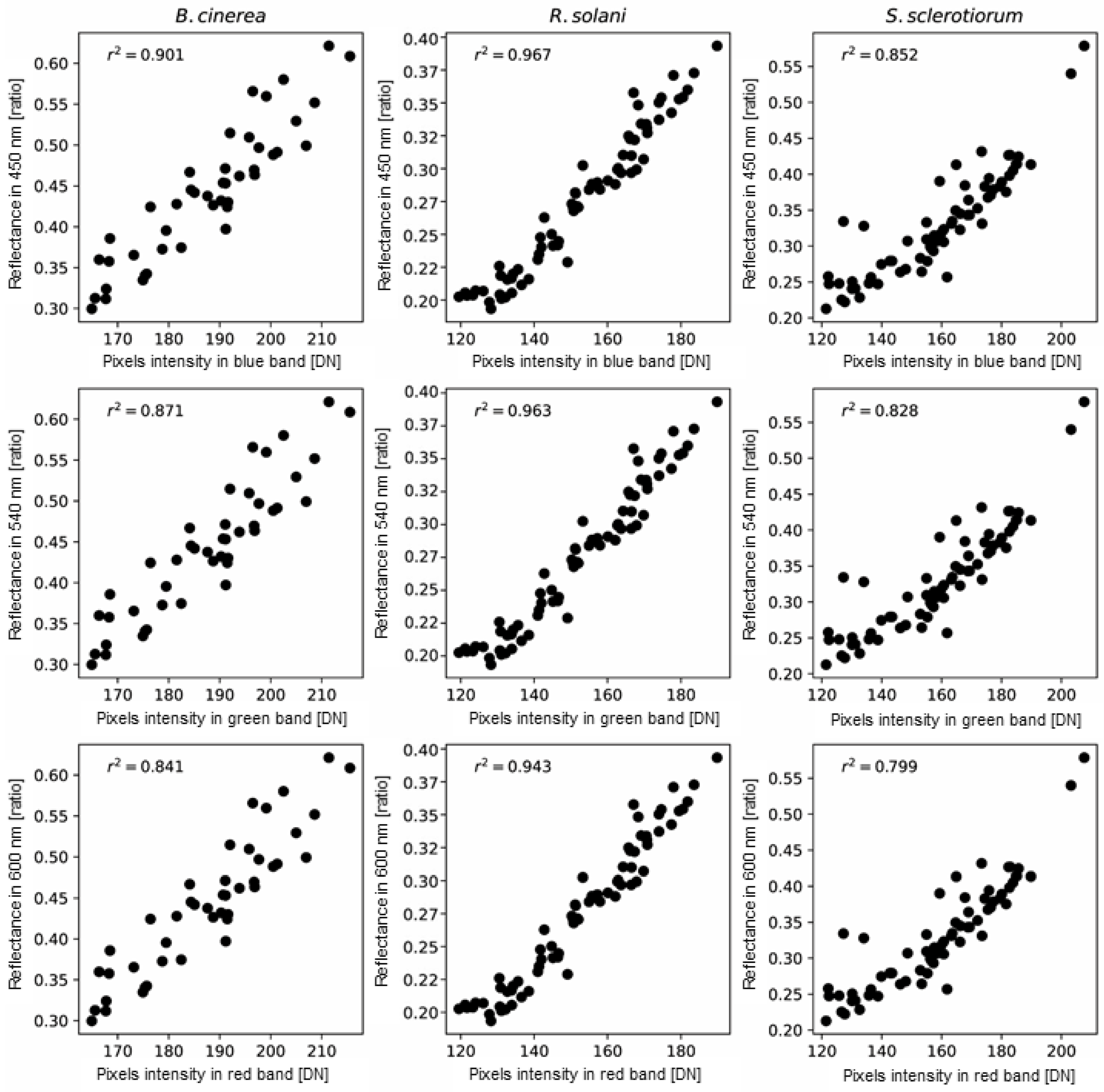
3.3. Relationship between Hyperspectral and RGB Characteristics

There have been many studies on pathogen-fungi identification in the literature; however, few studies have compared the performance of hyperspectral and RGB characteristics of fungi. Our study indicated a close relationship between the intensity of pixels in the visible range and the corresponding values of hyperspectral reflectance factors (Figure 6). The highest convergence was obtained for R. solani in all three ranges (blue 0.984, green 0.982 and red 0.971) and the smallest for S. sclerotiorum (blue 0.923, green 0.910, red 0.894). Mutual relations between the values registered with RGB and hyperspectral cameras were analysed, among others by Du et al. [68], who investigated the colour display of hyperspectral data with a single RGB composite. Similar experiments were performed by Magnusson et al. [69], who presented a method of transforming the visible spectral bands of hyperspectral images to the RGB colour space. On the other hand, there are studies focused on recovering high-quality hyperspectral images from RGB values [70,71,72,73]. The high correlation between the intensity of the pixels in the visible range and the corresponding values of the hyperspectral reflectance presented in our work is consistent with the results of the research presented above. We hope that this approach may result in replacing expensive hyperspectral devices with consumer-grade low-cost RGB cameras. Another opportunity to increase pathogen identification effectiveness is combining RGB and hyperspectral imaging with image analysis software [21,74,75,76].
The results of the investigation indicate that the proposed method is worth applying in further studies in fungi identification.

4. Conclusions

The conducted research gave the opportunity to distinguish the analysed fungi not only based on hyperspectral curves but also with RGB images. The most effective method in the hyperspectral identification of the fungi analysed turned out to be the PCA method, in which the average values of Rec and Acc for all three fungi were 0.96 and 0.93, respectively. The most valuable wavelengths for distinguishing B. cinerea-R. solani and B. cinerea-S. sclerotiorum were the wavelengths of the SWIR range and for distinguishing Rhizoctonia-Sclerotinia the wavelengths of the VIS range.
The high correlation in three ranges of the visible spectrum (blue, green and red) between the hyperspectral and multispectral data indicates the possibility of developing a simpler method of identifying fungi in Petri dishes. The method based on RGB images proved to be successful primarily for the identification of R. solani (rec = 0.90, acc = 0.79) and S. sclerotiorum (rec = 0.84, acc = 0.76). The most significant differences in the intensity of the pixels between B. cinerea and R. solani and R. solani and S. sclerotiorum occurred in the blue band and in distinguishing B. cinerea and S. sclerotiorum in the red band.
The results of research on the use of RGB images to identify fungi bring us closer to the development of a quick and non-contact method of identifying fungi based on the use of cheap sensors. The presented results indicate the need to include the analysis of normalized RGB images in subsequent studies, converted to HSI (hue, saturation, intensity) [55] and spectral indices [61,77]. Considerable improvement in the access to image data and increase in computational power implies the opportunity to fast develop new methods based on the fusion of image acquisition techniques with machine learning. The collection of RGB and hyperspectral data registered in this study in the current spectral library enables multiple uses of the stored data in future research.

Author Contributions

J.P., A.W. and M.W.: Conceptualization, Investigation, Writing-Original Draft Preparation, Writing-Review & Editing, K.S., N.Ł.-S., I.Ś. and K.P.: Data Curation, Resources, Investigation, J.J.: Methodology, Visualization, Writing-Original Draft Preparation. All authors have read and agreed to the published version of the manuscript.

Funding

This research received no external funding.

Institutional Review Board Statement

Not applicable.

Informed Consent Statement

Not applicable.

Data Availability Statement

The data presented in this study are available on request from the corresponding author.

Conflicts of Interest

The authors declare no conflict of interest.

References

  1. Karimi, K.; Arzanlou, M.; Pertot, I. Development of novel species-specific primers for the specific identification of Colletotrichum nymphaeae based on conventional PCR and LAMP techniques. Eur. J. Plant Pathol. 2020, 156, 463–475. [Google Scholar] [CrossRef]
  2. Baturo-Cieśniewska, A.; Groves, C.L.; Albrecht, K.A.; Grau, C.R.; Willis, D.K.; Smith, D.L. Molecular identification of Sclerotinia trifoliorum and Sclerotinia sclerotiorum isolates from the United States and Poland. Plant Dis. 2017, 101, 192–199. [Google Scholar] [CrossRef] [Green Version]
  3. Šišić, A.; Oberhänsli, T.; Baćanović-Šišić, J.; Hohmann, P.; Finckh, M.R. A novel real time PCR method for the detection and quantification of Didymella pinodella in symptomatic and asymptomatic plant hosts. J. Fungi 2022, 8, 41. [Google Scholar] [CrossRef] [PubMed]
  4. Pieczul, K.; Perek, A.; Kubiak, K. Detection of Tilletia caries, Tilletia laevis and Tilletia controversa wheat grain contamination using loop-mediated isothermal DNA amplification (LAMP). J. Microbiol. Methods 2018, 154, 141–146. [Google Scholar] [CrossRef] [PubMed]
  5. Baysal-Gurel, F.; Ivey, M.L.L.; Dorrance, A.; Luster, D.; Frederick, R.; Czarnecki, J.; Miller, S.A. An immunofluorescence assay to detect urediniospores of Phakopsora pachyrhizi. Plant Dis. 2008, 92, 1387–1393. [Google Scholar] [CrossRef] [Green Version]
  6. Milner, H.; Ji, P.; Sabula, M.; Wu, T. Quantitative polymerase chain reaction (Q-PCR) and fluorescent in situ hybridization (FISH) detection of soilborne pathogen Sclerotium rolfsii. Appl. Soil Ecol. 2019, 136, 86–92. [Google Scholar] [CrossRef]
  7. Thornton, C.R.; Slaughter, D.C.; Davis, R.M. Detection of the sour-rot pathogen Geotrichum candidum in tomato fruit and juice by using a highly specific monoclonal antibody-based ELISA. Int. J. Food Microbiol. 2010, 143, 166–172. [Google Scholar] [CrossRef] [Green Version]
  8. Prigione, V.; Lingua, G.; Marchisio, V.F. Development and use of flow cytometry for detection of airborne fungi. Appl. Environ. Microbiol. 2004, 70, 1360–1365. [Google Scholar] [CrossRef] [Green Version]
  9. Pan, L.; Zhang, W.; Zhu, N.; Mao, S.; Tu, K. Early detection and classification of pathogenic fungal disease in post-harvest strawberry fruit by electronic nose and gas chromatography–mass spectrometry. Food Res. Int. 2014, 62, 162–168. [Google Scholar] [CrossRef]
  10. Hariharan, G.; Prasannath, K. Recent advances in molecular diagnostics of fungal plant pathogens: A mini review. Front. Cell. Infect. Microbiol. 2021, 10, 600234. [Google Scholar] [CrossRef]
  11. D’Hondt, L.; Höfte, M.; Van Bockstaele, E.; Leus, L. Applications of flow cytometry in plant pathology for genome size determination, detection and physiological status. Mol. Plant Pathol. 2011, 12, 815–828. [Google Scholar] [CrossRef] [PubMed]
  12. Fang, Y.; Ramasamy, R.P. Current and prospective methods for plant disease detection. Biosensors 2015, 5, 537–561. [Google Scholar] [CrossRef] [PubMed] [Green Version]
  13. Gold, K.M.; Townsend, P.A.; Chlus, A.; Herrmann, I.; Couture, J.J.; Larson, E.R.; Gevens, A.J. Hyperspectral measurements enable pre-symptomatic detection and differentiation of contrasting physiological effects of late blight and early blight in potato. Remote Sens. 2020, 12, 286. [Google Scholar] [CrossRef] [Green Version]
  14. Sancho-Adamson, M.; Trillas, M.I.; Bort, J.; Fernandez-Gallego, J.A.; Romanyà, J. Use of RGB vegetation indexes in assessing early effects of Verticillium wilt of olive in asymptomatic plants in high and low fertility scenarios. Remote Sens. 2019, 11, 607. [Google Scholar] [CrossRef] [Green Version]
  15. Yao, Z.; Lei, Y.; He, D. Early visual detection of wheat stripe rust using visible/near-infrared hyperspectral imaging. Sensors 2019, 19, 952. [Google Scholar] [CrossRef] [Green Version]
  16. Yu, K.; Anderegg, J.; Mikaberidze, A.; Karisto, P.; Mascher, F.; McDonald, B.A.; Hund, A. Hyperspectral canopy sensing of wheat Septoria tritici blotch disease. Front. Plant Sci. 2018, 9, 1195. [Google Scholar] [CrossRef] [Green Version]
  17. Wijekoon, C.P.; Goodwin, P.H.; Hsiang, T. Quantifying fungal infection of plant leaves by digital image analysis using Scion Image software. J. Microbiol. Methods 2008, 74, 94–101. [Google Scholar] [CrossRef]
  18. Corkidi, G.; Balderas-Ruíz, K.A.; Taboada, B.; Serrano-Carreón, L.; Galindo, E. Assessing mango anthracnose using a new three-dimensional image-analysis technique to quantify lesions on fruit. Plant Pathol. 2006, 55, 250–257. [Google Scholar] [CrossRef]
  19. Thomas, S.; Kuska, M.T.; Bohnenkamp, D.; Brugger, A.; Alisaac, E.; Wahabzada, M.; Mahlein, A.K. Benefits of hyperspectral imaging for plant disease detection and plant protection: A technical perspective. J. Plant Dis. Prot. 2018, 125, 5–20. [Google Scholar] [CrossRef]
  20. Padmavathi, K.; Thangadurai, K. Implementation of RGB and grayscale images in plant leaves disease detection—Comparative study. Indian J. Sci. Technol. 2016, 9, 1–6. [Google Scholar] [CrossRef]
  21. Bock, C.H.; Poole, G.H.; Parker, P.E.; Gottwald, T.R. Plant disease severity estimated visually, by digital photography and image analysis, and by hyperspectral imaging. Crit. Rev. Plant Sci. 2010, 29, 59–107. [Google Scholar] [CrossRef]
  22. Abdullah, N.E.; Rahim, A.A.; Hashim, H.; Kamal, M.M. Classification of rubber tree leaf diseases using multilayer perceptron neural network. In Proceedings of the 2007 5th Student Conference on Research and Evelopment, Selangor, Malaysia, 11–12 December 2007; IEEE: Manhattan, NY, USA, 2007; pp. 1–6. [Google Scholar]
  23. Yu, H.; Cheng, X.; Chen, C.; Heidari, A.A.; Liu, J.; Cai, Z.; Chen, H. Apple leaf disease recognition method with improved residual network. Multimed Tools Appl. 2022, 81, 7759–7782. [Google Scholar] [CrossRef]
  24. Price, T.V.; Gross, R.; Wey, J.H.; Osborne, C.F. A comparison of visual and digital image-processing methods in quantifying the severity of coffee leaf rust (Hemileia vastatrix). Aust. J. Exp. Agric. 1993, 33, 97–101. [Google Scholar] [CrossRef]
  25. Tucker, C.C.; Chakraborty, S. Quantitative assessment of lesion characteristics and disease severity using digital image processing. J. Phytopathol. 1997, 145, 273–278. [Google Scholar] [CrossRef]
  26. Martin, D.P.; Rybicki, E.P. Microcomputer-based quantification of maize streak virus symptoms in zea mays. Phytopathology 1998, 88, 422–427. [Google Scholar] [CrossRef] [Green Version]
  27. Weizheng, S.; Yachun, W.; Zhanliang, C.; Hongda, W. Grading method of leaf spot disease based on image processing. In Proceedings of the 2008 International Conference on Computer Science and Software Engineering, Wuhan, China, 12–14 December 2008; IEEE: Manhattan, NY, USA, 2008; pp. 491–494. [Google Scholar]
  28. Camargo, A.; Smith, J.S. Image pattern classification for the identification of disease causing agents in plants. Comput. Electron. Agric. 2009, 66, 121–125. [Google Scholar] [CrossRef]
  29. Herrero-Latorre, C.; Barciela-García, J.; García-Martín, S.; Peña-Crecente, R.M. Detection and quantification of adulterations in aged wine using RGB digital images combined with multivariate chemometric techniques. Food Chem. X 2019, 3, 100046. [Google Scholar] [CrossRef]
  30. Schleder, G.R.; Padilha, A.C.M.; Acosta, C.M.; Costa, M.; Fazzio, A. From DFT to machine learning: Recent approaches to materials science–a review. J. Phys. Mater. 2019, 2, 032001. [Google Scholar] [CrossRef]
  31. van Dijk, A.D.J.; Kootstra, G.; Kruijer, W.; de Ridder, D. Machine learning in plant science and plant breeding. Iscience 2021, 24, 101890. [Google Scholar] [CrossRef]
  32. Bock, C.H.; Barbedo, J.G.; Del Ponte, E.M.; Bohnenkamp, D.; Mahlein, A.K. From visual estimates to fully automated sensor-based measurements of plant disease severity: Status and challenges for improving accuracy. Phytopathol. Res. 2020, 2, 9. [Google Scholar] [CrossRef] [Green Version]
  33. Singh, A.; Ganapathysubramanian, B.; Singh, A.K.; Sarkar, S. Machine learning for high-throughput stress phenotyping in plants. Trends Plant Sci. 2016, 21, 110–124. [Google Scholar] [CrossRef] [PubMed] [Green Version]
  34. Hesami, M.; Alizadeh, M.; Jones, A.M.P.; Torkamaneh, D. Machine learning: Its challenges and opportunities in plant system biology. Appl. Microbiol. Biotechnol. 2022, 106, 3507–3530. [Google Scholar] [CrossRef] [PubMed]
  35. Grinblat, G.L.; Uzal, L.C.; Larese, M.G.; Granitto, P.M. Deep learning for plant identification using vein morphological patterns. Comput. Electron. Agric. 2016, 127, 418–424. [Google Scholar] [CrossRef] [Green Version]
  36. Mishra, B.; Kumar, N.; Mukhtar, M.S. Systems biology and machine learning in plant–pathogen interactions. Mol. Plant-Microbe Interact. 2019, 32, 45–55. [Google Scholar] [CrossRef] [PubMed] [Green Version]
  37. Aboelghar, M.; Wahab, H.A. Spectral footprint of Botrytis cinerea, a novel way for fungal characterization. Adv. Biosci. Biotechnol. 2013, 4, 374–382. [Google Scholar] [CrossRef] [Green Version]
  38. Aboelghar, M.; Moustafa, M.S.; Ali, A.M.; Wahab, H.A. Hyperspectral analysis of Botrytis cinerea infected lettuce. EPH-Int. J. Agric. Environ. Res. 2019, 5, 26–42. [Google Scholar]
  39. Reynolds, G.J.; Windels, C.E.; MacRae, I.V.; Laguette, S. Hyperspectral remote sensing for detection of Rhizoctonia crown and root rot in sugarbeet. Phytopathology 2009, 99, 108. [Google Scholar]
  40. Cao, F.; Liu, F.; Guo, H.; Kong, W.; Zhang, C.; He, Y. Fast detection of Sclerotinia sclerotiorum on oilseed rape leaves using low-altitude remote sensing technology. Sensors 2018, 18, 4464. [Google Scholar] [CrossRef] [Green Version]
  41. Cameron, M.; Kumar, L. The Depths of Cast Shadow. Remote Sens. 2019, 11, 1806. [Google Scholar] [CrossRef] [Green Version]
  42. Piekarczyk, J.; Ratajkiewicz, H.; Jasiewicz, J.; Sosnowska, D.; Wójtowicz, A. An application of reflectance spectroscopy to differentiate of entomopathogenic fungi species. J. Photochem. Photobiol. B Biol. 2019, 190, 32–41. [Google Scholar] [CrossRef]
  43. Savitzky, A.; Golay, M.J.E. Smoothing and differentiation of data by simplified least squares procedures. Anal. Chem. 1964, 36, 1627–1639. [Google Scholar] [CrossRef]
  44. Chen, T.; Guestrin, C. XGBoost: A scalable tree boosting system. In Proceedings of the 22nd ACM SIGKDD International Conference on Knowledge Discovery and Data Mining, San Francisco, CA, USA, 13–17 August 2016; ACM: New York, NY, USA, 2016; pp. 785–794. [Google Scholar]
  45. Nawar, S.; Mouazen, A.M. Comparison between random forests, artificial neural networks and gradient boosted machines methods of on-line Vis-NIR spectroscopy measurements of soil total nitrogen and total carbon. Sensors 2017, 17, 2428. [Google Scholar] [CrossRef] [PubMed]
  46. Golden, C.E.; Rothrock, M.J., Jr.; Mishra, A. Comparison between random forest and gradient boosting machine methods for predicting Listeria spp. prevalence in the environment of pastured poultry farms. Food Res. Int. 2019, 122, 47–55. [Google Scholar] [CrossRef] [PubMed] [Green Version]
  47. dos Santos, U.J.; de Melo Dematte, J.A.; Menezes, R.S.C.; Dotto, A.C.; Guimarães, C.C.B.; Alves, B.J.R.; Primoa, D.C.; Sampaio, E.V.D.S.B. Predicting carbon and nitrogen by visible near-infrared (Vis-NIR) and mid-infrared (MIR) spectroscopy in soils of Northeast Brazil. Geoderma Reg. 2020, 23, e00333. [Google Scholar] [CrossRef]
  48. Ivanov, A.; Riccardi, G. Kolmogorov-Smirnov test for feature selection in emotion recognition from speech. In Proceedings of the 2012 IEEE International Conference on Acoustics, Speech and Signal Processing (ICASSP), Kyoto, Japan, 25–30 March 2012; IEEE: Manhattan, NY, USA, 2012; pp. 5125–5128. [Google Scholar]
  49. Japkowicz, N.; Shah, M. Evaluating Learning Algorithms: A Classification Perspective; Cambridge University Press: Cambridge, UK, 2011. [Google Scholar]
  50. Fabris, F.; Freitas, A.A. Analysing the Overfit of the Auto-sklearn Automated Machine Learning Tool; ACM: Nicosia, Cyprus, 2019. [Google Scholar]
  51. Tsamardinos, I.; Greasidou, E.; Borboudakis, G. Bootstrapping the out-of-sample predictions for efficient and accurate cross-validation. Mach. Learn. 2018, 107, 1895–1922. [Google Scholar] [CrossRef] [Green Version]
  52. Pituch, K.A.; Stapleton, L.M.; Kang, J.Y. A comparison of single sample and bootstrap methods to assess mediation in cluster randomized trials. Multivar. Behav. Res. 2006, 41, 367–400. [Google Scholar] [CrossRef]
  53. Conrad, A.O.; Li, W.; Lee, D.Y.; Wang, G.L.; Rodriguez-Saona, L.; Bonello, P. Machine learning-based presymptomatic detection of rice sheath blight using spectral profiles. Plant Phenomics 2020, 2020, 8954085. [Google Scholar] [CrossRef]
  54. Kong, W.; Zhang, C.; Huang, W.; Liu, F.; He, Y. Application of hyperspectral imaging to detect Sclerotinia sclerotiorum on oilseed rape stems. Sensors 2018, 18, 123. [Google Scholar] [CrossRef] [Green Version]
  55. Cambaza, E.; Koseki, S.; Kawamura, S. Why RGB imaging should be used to analyze Fusarium graminearum growth and estimate deoxynivalenol contamination. Methods Protoc. 2019, 2, 25. [Google Scholar] [CrossRef] [Green Version]
  56. Ponti, M.; Chaves, A.A.; Jorge, F.R.; Costa, G.B.; Colturato, A.; Branco, K.R. Precision agriculture: Using low-cost systems to acquire low-altitude images. IEEE Comput. Graph. Appl. 2016, 36, 14–20. [Google Scholar] [CrossRef]
  57. Zhang, S.; Wu, X.; You, Z.; Zhang, L. Leaf image based cucumber disease recognition using sparse representation classification. Comput. Electron. Agric. 2017, 134, 135–141. [Google Scholar] [CrossRef]
  58. Zhang, S.; Zhang, S.; Zhang, C.; Wang, X.; Shi, Y. Cucumber leaf disease identification with global pooling dilated convolutional neural network. Comput. Electron. Agric. 2019, 162, 422–430. [Google Scholar] [CrossRef]
  59. Kumar, R.; Baloch, G.; Pankaj, A.B.B.; Abdul, B.B.; Bhatti, J. Fungal blast disease detection in rice seed using machine learning. Int. J. Adv. Comput. Sci. Appl. 2021, 12, 248–258. [Google Scholar] [CrossRef]
  60. Fernández, C.I.; Leblon, B.; Wang, J.; Haddadi, A.; Wang, K. Detecting infected cucumber plants with close-range multispectral imagery. Remote Sens. 2021, 13, 2948. [Google Scholar] [CrossRef]
  61. Pozza, E.A.; de Carvalho Alves, M.; Sanches, L. Using computer vision to identify seed-borne fungi and other targets associated with common bean seeds based on red–green–blue spectral data. Trop. Plant Pathol. 2022, 47, 168–185. [Google Scholar] [CrossRef]
  62. Anthonys, G.; Wickramarachchi, N. An image recognition system for crop disease identification of paddy fields in Sri Lanka. In Proceedings of the 2009 International Conference on Industrial and Information Systems (ICIIS), Peradeniya, Sri Lanka, 28–31 December 2009; IEEE: Manhattan, NY, USA, 2009; pp. 403–407. [Google Scholar]
  63. Pavicic, M.; Overmyer, K.; Rehman, A.; Jones, P.; Jacobson, D.; Himanen, K. Image-based methods to score fungal pathogen symptom progression and severity in excised Arabidopsis leaves. Plants 2021, 10, 158. [Google Scholar] [CrossRef]
  64. Sun, Y.; Gu, X.; Wang, Z.; Huang, Y.; Wei, Y.; Zhang, M.; Tu, K. Leiqing Pan Growth simulation and discrimination of Botrytis cinerea, Rhizopus stolonifer and Colletotrichum acutatum using hyperspectral reflectance imaging. PLoS ONE 2015, 10, e0143400. [Google Scholar]
  65. Zhou, X.G.; Zhang, D.; Lin, F. UAV remote sensing: An innovative tool for detection and management of rice diseases. In Diagnostics of Plant Diseases; Kurouski, D., Ed.; IntechOpen: London, UK, 2021; p. 95535. [Google Scholar]
  66. Rego, C.H.Q.; França-Silva, F.; Gomes-Junior, F.G.; Moraes, M.H.D.D.; Medeiros, A.D.D.; Silva, C.B.D. Using multispectral imaging for detecting seed-borne fungi in cowpea. Agriculture 2020, 10, 361. [Google Scholar] [CrossRef]
  67. Fahrentrapp, J.; Ria, F.; Geilhausen, M.; Panassiti, B. Detection of gray mold leaf infections prior to visual symptom appearance using a five-band multispectral sensor. Front. Plant Sci. 2019, 10, 628. [Google Scholar] [CrossRef] [Green Version]
  68. Du, Q.; Raksuntorn, N.; Cai, S.; Moorhead, R.J. Color display for hyperspectral imagery. IEEE Trans. Geosci. Remote Sens. 2008, 46, 1858–1866. [Google Scholar] [CrossRef]
  69. Magnusson, M.; Sigurdsson, J.; Armansson, S.E.; Ulfarsson, M.O.; Deborah, H.; Sveinsson, J.R. Creating RGB images from hyperspectral images using a color matching function. In Proceedings of the IGARSS 2020-2020 IEEE International Geoscience and Remote Sensing Symposium, Waikoloa, HI, USA, 26 September–2 October 2020; IEEE: Manhattan, NY, USA, 2020; pp. 2045–2048. [Google Scholar]
  70. Cao, X.; Tong, X.; Dai, Q.; Lin, S. High resolution multispectral video capture with a hybrid camera system. In Proceedings of the CVPR 2011, Colorado Springs, CO, USA, 20–25 June 2011; IEEE: Manhattan, NY, USA, 2011; pp. 297–304. [Google Scholar]
  71. Kawakami, R.; Matsushita, Y.; Wright, J.; Ben-Ezra, M.; Tai, Y.W.; Ikeuchi, K. High-resolution hyperspectral imaging via matrix factorization. In Proceedings of the CVPR 2011, Colorado Springs, CO, USA, 20–25 June 2011; IEEE: Manhattan, NY, USA, 2011; pp. 2329–2336. [Google Scholar]
  72. Arad, B.; Ben-Shahar, O. Sparse recovery of hyperspectral signal from natural RGB images. In European Conference on Computer Vision; Leibe, B., Matas, J., Sebe, N., Welling, M., Eds.; Springer: Berlin/Heidelberg, Germany, 2016; pp. 19–34. [Google Scholar]
  73. Shi, Z.; Chen, C.; Xiong, Z.; Liu, D.; Wu, F.H. Advanced cnn-based hyperspectral recovery from RGB images. In Proceedings of the IEEE Conference on Computer Vision and Pattern Recognition Workshops, Salt Lake City, UT, USA, 18–22 June 2018; IEEE: Manhattan, NY, USA, 2018; pp. 939–947. [Google Scholar]
  74. Barbedo, J.G.A. Digital image processing techniques for detecting, quantifying and classifying plant diseases. SpringerPlus 2013, 2, 660. [Google Scholar] [CrossRef] [PubMed] [Green Version]
  75. Bardsley, S.J.; Ngugi, H.K. Reliability and accuracy of visual methods to quantify severity of foliar bacterial spot symptoms on peach and nectarine. Plant Pathol. 2013, 62, 460–474. [Google Scholar] [CrossRef]
  76. Abd-El-Haliem, A. An unbiased method for the quantitation of disease phenotypes using a custom-built macro plugin for the program ImageJ. In Plant Fungal Pathogens. Methods in Molecular Biology (Methods and Protocols), Bolton, M., Thomma, B., Eds.; Humana Press: New York, NY, USA, 2012; pp. 635–644. [Google Scholar]
  77. Hunt, E.R., Jr.; Daughtry, C.S.T.; Eitel, J.U.; Long, D.S. Remote sensing leaf chlorophyll content using a visible band index. Agron. J. 2011, 103, 1090–1099. [Google Scholar] [CrossRef] [Green Version]
Figure 1. Three species of fungal cultures on Petri dishes.
Agronomy 12 01965 g001
Figure 2. Data processing procedure.
Agronomy 12 01965 g002
Figure 3. Mean spectra of three fungi species: B. cinerea, R. solani, S. sclerotiorum.
Agronomy 12 01965 g003
Figure 4. Comparison of the spectra of three fungi species. The 10 wavelengths most useful for distinguishing the three fungi species are marked by dashed vertical lines.
Agronomy 12 01965 g004
Figure 5. Distinguishing between three species of fungi based on the intensity of pixels in three spectral bands from an RGB images.
Agronomy 12 01965 g005
Figure 6. Relationships between the reflectance of the three wavelengths 450, 540, 600 nm and the average intensity of the pixels from the three RGB channels (red, green, blue) (p-value for all r2 < 10−16).
Agronomy 12 01965 g006
Table 1. The 10 wavelengths most useful for distinguishing the three fungi species based on the values D-statistic.
B. cinerea-R. solaniB. cinerea-S. sclerotiorumR. solani-S. sclerotiorum
BandD-StatisticBandD-StatisticBandD-Statistic
19040.79119040.8185720.525
19060.78913760.8155750.511
13820.78919010.8005630.496
18990.77914200.7995760.475
19030.77618990.7985640.458
13760.77513730.7985930.437
18610.77318970.7975590.433
13780.77218680.79410020.430
13750.77019030.7905920.412
13830.77018670.78811410.394
Table 2. Reliability of distinguishing three species of fungi on the basis of hyperspectral data.
MethodsClassification AssesmentB. cinereaR. solaniS. sclerotiorumMean
All featuresWrong a9186
Vague b11133921
Good c160270237222.333
Rec d0.9150.9670.9180.933
Acc e0.8890.9510.8350.891
Selected feturesWrong861810.667
Vague15293626.667
Good157249230212
Rec0.9040.9220.8740.900
Acc0.8720.8770.8100.853
PCAWrong6545
Vague11131111,667
Good163266269232.667
Rec0.9400.9620.9630.955
Acc0.9100.9400.9500.933
a incorrectly classified if the outcome shows a different label than the actual, but steady, namely, more than 85% hits for a wrong case. b if outcome takes different labels at each iteration. c correctly classified if the outcome agrees with the actual in more than 85% hits. d the ratio of correctly classified objects to the total number of control objects in this class. e the ratio of correctly classified objects to the total number of classified objects in this class.
Table 3. Reliability in distinguishing three species of fungi based on RGB images.
Classification AssesmentB. cinereaR. solaniS. sclerotiorum
Wrong a615
Vague b161412
Good c235754
Rec d0.7170.8980.835
Acc e0.5110.7920.761
Markings a, b, c, d, e as in the Table 2.
Publisher’s Note: MDPI stays neutral with regard to jurisdictional claims in published maps and institutional affiliations.

