Article

How Well Can Reflectance Spectroscopy Allocate Samples to Soil Fertility Classes?

1
School of Geography Science, Nanjing University of Information Science and Technology, Nanjing 210044, China
2
State Key Laboratory of Soil and Sustainable Agriculture, Institute of Soil Science, Chinese Academy of Sciences, Nanjing 210008, China
3
Section of Soil and Crop Sciences, Cornell University, Ithaca, NY 14853, USA
4
ISRIC-World Soil Information, 6700 AJ Wageningen, The Netherlands
5
Upland Flue-Cured Tobacco Quality & Ecology Key Laboratory of China Tobacco Guizhou Academy of Tobacco Science, Guiyang 550081, China
6
College of Resources and Environment, Southwest University, Chongqing 400715, China
7
China National Tobacco Corporation Guizhou Provincial Company, Guiyang 550004, China
*
Author to whom correspondence should be addressed.
Agronomy 2022, 12(8), 1964; https://doi.org/10.3390/agronomy12081964
Submission received: 20 July 2022 / Revised: 12 August 2022 / Accepted: 17 August 2022 / Published: 20 August 2022
(This article belongs to the Special Issue Soil Sustainability in the Anthropocene)

Abstract

:
Fertilization decisions depend on the measurement of a large set of soil fertility indicators, usually through laboratory determination, which is costly and time-consuming. Visible and near-infrared (vis-NIR) spectroscopy combined with machine learning can simultaneously predict various soil fertility indicators. Spectroscopy is inherently less accurate than direct laboratory determination. However, in many fertilization recommendation contexts, farmers mainly fertilize according to classified fertility indicators, rather than by continuous soil property values. These classes have defined limits of property values. We hypothesized that the additional inaccuracy from spectroscopy may not be important for properties grouped into classes. This study compared the indirect and direct prediction of soil fertility classes. Indirectly, by (1) using vis-NIR spectra with machine learning to predict 20 soil fertility indicators (pH, soil organic matter (SOM), cation exchange capacity (CEC), total nitrogen (TN), total phosphorus (TP), total potassium (TK), alkali-hydrolyzable nitrogen (AN), available phosphorus (AP), available potassium (AK), calcium (Ca), magnesium (Mg), silicon (Si), sulfur (S), boron (B), iron (Fe), manganese (Mn), copper (Cu), Zinc (Zn), molybdenum (Mo) and chlorine (Cl)) and (2) allocating the indicators to soil fertility classes. Directly, by predicting soil fertility classes directly from vis-NIR spectra using machine learning. The prediction accuracy of these two methods were compared and the accuracies needed for the acceptable class allocation of the fertility indicators were determined. The example dataset is a soil spectral library from the Guizhou Province, southwest China. The model performance was evaluated by the overall allocation accuracy and tau index, which accounts for class imbalance. For direct allocation based on three fertility classes (low, medium and high), the overall allocation accuracy of eight properties (CEC, Cu, Si, Zn, S, Mn, Ca and Mg), nine properties (B, AN, TK, AK, SOM, TN, TP, Fe and Mo) and three properties (Cl, AP and pH) were within the range of 0.80–1.0, 0.60–0.80 and 0.40–0.60, respectively. For indirect allocation based on the same classes, the allocation accuracy of nine properties (TN, CEC, Cu, S, Zn, Si, Mn, Ca and Mg), nine properties (B, TK, pH, TP, AK, AN, Fe, Mo and SOM) and two properties (Cl and AP) were within the range of 0.80–1.0, 0.60–0.80 and 0.40–0.60, respectively. We conclude that vis-NIR spectroscopy was fairly successful for soil fertility class allocation for most of the soil properties, using either direct or indirect models. The advantage of indirect models is that both specific property values and soil fertility classes can be obtained at no increase in cost, while direct models are suggested when only soil fertility class information are available.

1. Introduction

Soil fertility has been defined as “the capacity of a soil to provide plants with nutrients” [1]. It is a comprehensive measure of soil functions to sustain the chemical status of the soil for proper crop growth, yield and quality. Soil fertility is generally evaluated by a set of indicators relevant to plant growth and quality, usually including pH, organic matter, cation exchange capacity (CEC), macronutrients and micronutrients [2,3]. Agricultural production consumes a large quantity of soil nutrient elements, which often need to be supplemented in the form of chemical fertilizers in order to maintain both quantity and quality of production.
Although fertilizer recommendations may be on a continuous scale, in many, if not most, recommendation domains, farmers fertilize according to classes of fertility indicators (e.g., three levels of “low”, “medium” and “high” [4] or five levels of “extremely low”, “low”, “medium”, “high” and “extremely high” [5]), defined by specified limits of the soil property values. Although precision agriculture is becoming more common, it is not much used by most of the world’s small and medium farmers, who manage on the basis of fertility classes. This is the case in the study area used in this research. These class determinations should be correct, so that stakeholders may take correct decisions. Yet all methods to measure soil fertility are uncertain, from field sampling through laboratory determination. The question is, how serious are these uncertainties when the measurements are grouped into classes relevant for soil management?
Although the laboratory determination of soil fertility indicators is accurate within laboratory experimental conditions, it is complicated, time-consuming, labor-intensive and costly. Thus, it is difficult to efficiently obtain soil fertility information for the large number of farmers served by a typical laboratory. The rapid development of visible and near-infrared (vis-NIR) spectroscopy promises to provides a solution for this [6,7]. The soil spectrum is a comprehensive integration of various physical and chemical properties of soil. Combined with the spectral library and machine learning methods, it can predict various soil fertility indicators simultaneously [8]. Although spectroscopy is inherently less accurate than direct physical and chemical laboratory determinations [9], due to the extra step of an imprecise model from spectra to property, this additional inaccuracy may not be important for properties grouped into classes. Further, although spectroscopy may not be able to directly detect some chemical species, especially heavy metals [10], correlative approaches have proven successful for many soil properties not directly related to spectral response [11,12,13].
Previous studies have mainly focused on the accuracy of spectroscopic models to predict soil fertility indicators and explored the use of different spectroscopic preprocessing methods, calibration set selection and modeling methods to improve prediction accuracy [8]. However, the correct allocation of classes for soil fertility indicators does not require the precision to be as high as possible, because soil fertility values within a certain range are categorized in the same class.
The prediction accuracy of different soil fertility indicators varies considerably, depending on the spectral responses of the target property, the spectral processing method, the prediction models used and the specific research areas [14,15,16]. In addition, there are many measures of prediction model success. The coefficient of determination (R2), root mean squared error (RMSE), relative percentage deviation (RPD) and the ratio of performance to the inter quartile distance (RPIQ) are commonly used to evaluate the prediction accuracy. Different criteria have been proposed to categorize the model performances. For example, according to Chang et al. [17], an RPD less than 1.4 indicates that the model is quite poor at estimating the property of interest, an RPD between 1.4 and 2.0 indicates that the model can roughly estimate the property of interest and an RPD greater than 2.0 indicates that the model can predict the property of interest with good accuracy. However, these criteria are based on continuous predicted and actual values, not on classes. For these, class-based accuracy measures should be used.
From the above, it seems that the large-scale and rapid allocation of soil samples to soil fertility classes with sufficient accuracy for practical application may be possible. Recently, a lot of research has explored using spectra directly or indirectly to predict soil fertility or soil quality indices [18,19,20,21]. These indices offer the integral evaluation of soil fertility or quality, and are calculated based on a selected set of key indicators. Viscarra Rossel, Rizzo, Demattê and Behrens [18] developed a soil fertility index using four soil properties (clay, CEC, base saturation and organic matter) and predicted the defined three soil fertility classes combing vis-NIR spectra and terrain attributes. The allocation accuracy of the fertility classes varied from 61% to 75%. Askari, O’Rourke and Holden [19] constructed two soil quality indices for agricultural production under grassland and arable land management and predicted these directly using spectra and indirectly by first inferring the quality indicators. The indices estimated directly from the soil spectra were more accurate than the indirect estimation. However, these researches did not explore the relationship between the prediction accuracy of soil fertility- or quality-related properties and the allocation accuracy to soil fertility classes. This is especially relevant when spectroscopy, rather than the more precise laboratory measurements, are used for property determination and allocation.
Therefore, we designed this study to compare the indirect and direct prediction of the soil fertility classes. Indirectly: (1) first predict 20 soil fertility indicators using vis-NIR spectra with machine learning, then (2) classify these according to user-defined class limits. Directly: predict the soil fertility classes of the 20 indicators directly from vis-NIR spectra using machine learning. Finally, compare the allocation accuracy of the two methods and propose the model accuracy needed for the practical class allocation of different fertility indicators. Finally, from this, determine which properties can be successfully allocated and recommend the best procedures for the allocation of soil samples into fertility classes.

2. Material and Methods

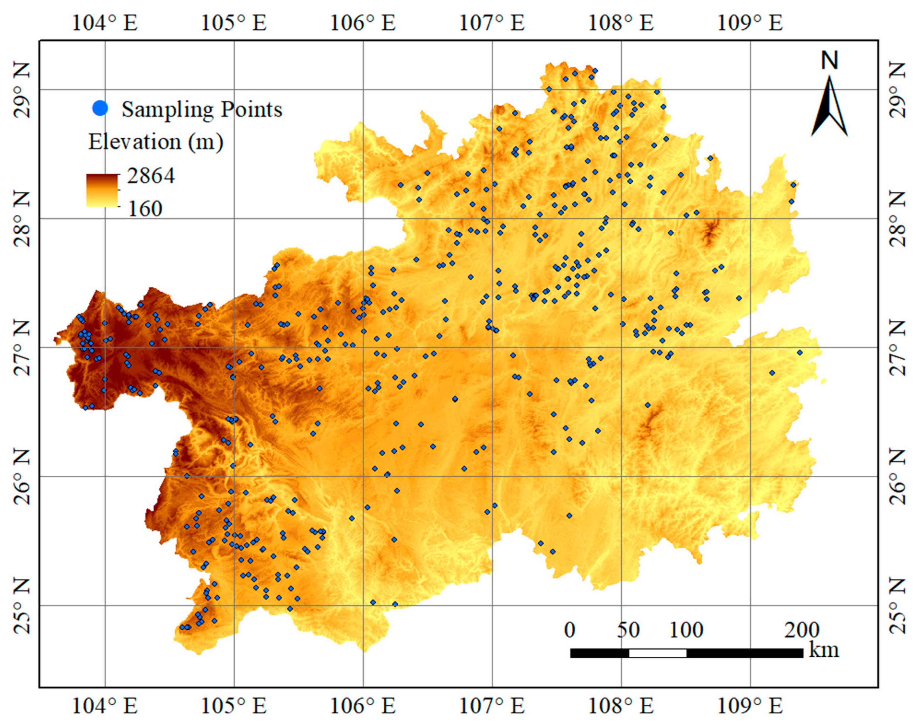
2.1. Research Area and Sampling

This study used a soil spectral library from Guizhou province, southwest China. Guizhou is in the subtropical humid climate zone, with an average annual precipitation from 850–1300 mm. The main landforms are mountains and hills. The major soil types are Histosols, Anthrosols, Gleyosols, Isohumosols, Ferrosols, Argosols, Cambosols and Primosols, based on the Chinese Soil Taxonomy [22]. The approximate correspondence to World Reference Base for Soil Resources [23] classes were listed in Supplementary Table S1. Five hundred and two (502) sampling points were located to represent different soil geographic environments used for dryland agriculture (Figure 1). Soil samples were collected from November to December in 2019. The land use is mainly a non-irrigated rotation of tobacco and maize. At each sampling point, five to eight nearby points were selected from the top layer (0–20 cm) to form a bulked sample. About 1.5 kg of soil per point was brought to the laboratory for analysis.

2.2. Laboratory Analysis and Spectroscopy

Twenty soil fertility indicators were measured by standard laboratory procedures [24], including pH, soil organic matter (SOM), cation exchange capacity (CEC), total nitrogen (TN), total phosphorus (TP), total potassium (TK), alkali-hydrolyzable nitrogen (AN), available phosphorus (AP), available potassium (AK), calcium (Ca), magnesium (Mg), silicon (Si), sulfur (S), boron (B), iron (Fe), manganese (Mn), copper (Cu), zinc (Zn), molybdenum (Mo) and chlorine (Cl).
Before spectra measurements, soil samples were air-dried and ground to pass 60-mesh (0.25 mm) sieve, then oven-dried at 45 °C for 24 h to remove the influence of soil moisture. Soil diffuse reflectance spectra (350~2500 nm) were collected using the Cary 5000 spectrometer. The spectral resolution was 0.048 nm for the range of 350~700 nm and 0.2 nm for the range of 700–2500 nm. Soil spectra were resampled to 1 nm. To reduce noise and enhance spectra features, soil spectra were subjected to Savitzky-Golay 1st order derivative and smoothing [25]. The smoothed spectra were averaged every 10 nm to reduce data redundancy.

2.3. Machine Learning Methods

In the indirect method, partial least square regression (PLSR) was used for prediction of the 20 soil fertility indicators. This is the most widely used chemometric method [26]. Prior to selecting PLSR, we compared the prediction accuracy of PLSR models with two other commonly used machine learning methods used in spectroscopy (Support Vector Machine (SVM) and Random Forest (RF), results not shown). This comparison revealed that in our study, there was no single best algorithm for all properties and that PLSR models were slightly better and more stable. PLSR models also require limited parameter tuning.
To avoid the randomness in division of calibration and validation set, a full cross validation strategy was adopted. Spectra preprocessing and PLSR models were processed in R 3.5.3 [27]. The accuracy of the PLSR models was evaluated by the coefficient of determination for cross validation (R2), root mean squared error (RMSE) and the ration of performance to inter quartile distance (RPIQ). These measures were used to evaluate the prediction accuracy of the 20 soil fertility indicators. Note that these are not yet indicators of class allocation, rather, of the continuous fertility indicators. The formulas of R2, RMSE and RPIQ are as followed:
R 2 = 1 i = 1 n ( y i y ^ ) / i = 1 n ( y i y ¯ ) 2
R M S E = 1 n i = 1 n ( y i y i ^ ) 2
RPIQ = IQ/RMSE
where n is the number of samples, y i is the measured value of soil fertility indicators, y ¯ is the average of the measured values, y i   ^   is the predicted value of soil fertility indicators and IQ is the inter-quartile range of the measured values.
These indicators each have an interpretation. R2 shows the proportion of the total variation in the sample set accounted for by the PLSR model. The RMSE is a summary for how close the predicted values are to the actual values. The RPIQ is the variability standardized by the average prediction error: a higher variability in the sample set allows for a larger prediction error. These indicators evaluate the continuous prediction model, but in this study the relevant evaluation is of the classified predictions.
In the direct method, two commonly used machine learning algorithms, namely Random Forest (RF) and Support Vector Machine [28] were used to predict the soil fertility class directly from spectra. These were trained on the classified values of the laboratory results, which were taken as correct, as they are so used in traditional fertility recommendations. These models were built with R packages ranger (RF) and e1071 (SVM). Although many other machine learning models could have been used, results from digital soil mapping classification, e.g., Brungard et al. [29], show that RF is consistently among the most accurate classifiers. The tuning of parameters for RF models was determined by using the caret package. SVM was successfully used to predict classes from spectra by Chen et al. [30], so this was used as an alternative. The commonly used radial basis function kernel was used for construction of SVM models. It is well-known that some of the indicators, especially heavy metals, do not have a direct spectral signature [10]. However, because of correlations with soil properties that do have signatures, it may be possible in a restricted geographical area, e.g., a soil fertility recommendation domain such as dryland tobacco and maize in Guizhou, to satisfactorily allocate even these to classes. This was to be tested by this study.

2.4. Class Allocation of Soil Fertility Indicators

A standard fertility indicator classification for arable land under the rotation of tobacco and maize in Guizhou province is split into five classes: extremely low, low, medium, high and extremely high, according to the criteria presented in Table 1 [31]. These criteria were determined according to the local fertilization management practices, as well as the definition of soil fertility classes and their limits in Guizhou Province and surrounding areas. These limits are widely used for fertilizer recommendations and, therefore, make a suitable basis for this study. The allocation accuracy statistics are highly dependent on the number of classes and their limits. Here, we have a practical example which represents similar situations worldwide.

2.5. Model Evaluation

The predicted soil fertility indicators based on PLSR models were used to determine the fertility class and then compared with the class determined based on observed values. This resulted in a confusion matrix, also called a cross-classification matrix, of the predicted versus the observed fertility class. The confusion matrix is a table of the predicted class versus the observed class, which can visually present the correct allocation as well as the misallocation. The allocation accuracy of soil fertility class was evaluated using the overall allocation accuracy, the user’s accuracy [32] and tau index [33]. The overall allocation accuracy summarizes the number of samples correctly allocated and divide by the total number of samples. The user’s accuracy shows how well the allocation performed, from the point of view of the user. The tau index was developed as a replacement for the well-known deprecated kappa coefficient [34], to measure how the allocation compares to random assignment. That is, it measures the skill of the allocator and accounts for the size of each class and its prior probability as known by the allocator, in this case, the allocation algorithm.
The cross-classification matrix is the fundamental data structure in accuracy assessment [32]. As explained in Rossiter et al. [35], it is constructed as follows. Given n samples that have been allocated to r classes, labelled i = 1, 2……r, we set up a square asymmetric matrix r × r, in which each row and column corresponds to one class, in the same order. In each cell Xij, we enter the number of samples which are of class j that have been predicted to belong to class i. The diagonal entries X11, X22,……Xrr represent agreement between predicted and actual and the off-diagonals represent misallocations.
From this matrix we compute row sums Xi+, i.e., the total number allocated to class i, and the column sums X+j, i.e., the total actually in class j. The row-wise proportion of correct allocations UAi = Xii/Xi+ is commonly known as the “user’s accuracy” for class i. The column-wise proportion of correct allocations PAj = Xjj/X+j is commonly known as the “producer’s accuracy” for class j. The overall allocation accuracy is   O A = i = 1 r X i i / n   , the proportion of all samples correctly allocated.
The tau index is calculated as follows:
t a u = O A θ 1 1 θ 1
where   θ 1 = i = 1 r X i X + i , Xi is the prior probabilities for soil fertility class i.
We calculated tau based on different prior probabilities: tau1 based on equal prior probabilities (i.e., ignorance of the class distribution) and tau2 based on the proportions in the reference set (i.e., complete knowledge of expected proportions). Calculations were with the tauW function of the aqp (Algorithms for Quantitative Pedology) R package [36,37].
Five classes of soil fertility may be too fine a distinction in many cases for providing guidance in soil nutrients management. In many practical situations, three classes (low, medium and high) or even only two classes (sufficient or deficient) are needed in practice [38]. Thus, the class of “extremely low” and “low” were combined as “low”, while the class of “extremely high” and “high” were combined as “high”. The confusion matrix and the prediction accuracy were also established for the three fertility classes, in comparison to the criteria of five classes.

3. Results and Discussion

3.1. Summary Characteristics of the Soil Fertility Indicators

Table 2 and Table 3 show the statistical summary of the 20 soil fertility indicators and the proportion of these in each fertility class, respectively. Table 2 shows that only Cl had a high coefficient of variation (CV > 100%), the other 19 soil properties all fell within the range of moderate variation (CV: 10–100%). Mn and pH had a negatively skewed distribution (skewness < 0), while the remaining properties were all positively skewed in their distribution (skewness > 0). Four indicators of pH, Mn, S and P had flat-topped distributions (kurtosis < 0) and the remaining 16 indicators had sharp-peak distributions (kurtosis > 0).
According to the summary statistics of soil fertility classes and the established class limits for the research area, the sampled soils were relatively rich in the contents of SOM, CEC, TN, AN, AK, Si, S, B, Fe, Mn, Cu, Zn and Mo, with the proportion of the soil fertility class being no less than “medium” (sum of “medium”, “high” and “extremely high”), exceeding 80% (83–97%). The contents of TP, TK, Ca, Mg, Cl and AP were relatively deficient, e.g., for Ca, about 97.21% belonged to the class of “low” or “extremely low”. For soil pH, about 42.83% were in the suitable range (medium), about 36.85% was relatively high (high and extremely high) for crop growth, while 20.30% was relatively low (low and extremely low).
Table 3 clearly reveals the imbalance in class allocation; however, this is not consistent across properties. For example, about two-thirds of the samples were in the “medium” total N class, whereas almost four-fifths of the samples were in the “very low” Ca class. This motivates the use of the tau index, rather than simply the overall allocation accuracy, to evaluate the skill of the allocation method.

3.2. Prediction Accuracy of PLSR Models

The prediction accuracy of soil fertility indicators by PLSR models is presented in Table 4. Following the criteria suggested by Chang, Laird, Mausbach and Hurburgh [17], no fertility indicators satisfied the category of good performance. Only seven soil properties (pH, SOM, CEC, TN, TK, Mg and Si) achieved moderate prediction performances, with R2 ranging from 0.518 to 0.626 and RPIQ ranging from 1.744 to 2.796. The prediction accuracy of the remaining 13 soil properties were all poor (R2: 0.012 to 0.461, RPIQ: 0.543 to 1.692). As expected, the heavy metals were especially poorly-predicted. However, this is the accuracy evaluated as a continuous property, not as classes, which is our aim.
Soil properties can be predicted by vis-NIR spectroscopy based on either their direct spectral responses or their correlations to soil properties with direct spectral responses. The relatively high prediction accuracy of SOM and TN was expected because their molecular bonds have direct spectral responses in the vis-NIR regions. Some other soil properties (pH, CEC, TK, Mg and Si) without direct spectral responses can still be predicted with moderate accuracy, likely due to their correlation with spectrally-active constituents, such as SOM, TN and particle size [39]. The relatively high prediction accuracy achieved by the available Mg was also reported by Mouazen et al. [40]. They explained that this might be due to the strong correlation between the total Mg and the near infrared spectra as well the close relationship between the total and available Mg. Most of the micronutrients were poorly predicted, mainly due to their relatively low concentrations and lack of direct spectral response [41].
As suggested by Chang, Laird, Mausbach and Hurburgh [17], the soil properties with a moderate prediction accuracy have the potential to be improved by varied calibration strategies, while properties with poor accuracy may not be reliably predicted by spectroscopy. The question is, can we still extract useful information, in this case, proper fertilizer recommendations, from these poorly-predicted models of soil properties once the predictions are grouped into user-defined classes?

3.3. Allocation of Soil Fertility Classes Indirectly from Spectra

3.3.1. Allocation Based on Five Fertility Classes

Table 5 shows the evaluation statistics for the fertility class allocation. Mg, Si and Mn achieved a high overall allocation accuracy (0.863–0.876). This is a good result, considering that their prediction accuracy by PSLR models were only moderate (R2: 0.288–0.571, RPIQ: 1.692–2.295). The allocation accuracy of SOM, CEC, TN, TP, AN, Ca, S and Zn were within the range of 0.60–0.80, still better than their prediction accuracy, which was 0.046–0.626 for R2 and 0.638–2.192 for RPIQ. The remaining nine soil properties (pH, TK, AP, AK, B, Fe, Cu, Mo and Cl) achieved an allocation accuracy of less than 0.60 (0.239–0.584). Interestingly, the soil properties predicted more accurately (higher RPIQ) do not always result in a high allocation accuracy (e.g., pH and CEC), while relatively poorly predicted properties can also achieve a high allocation accuracy (e.g., Mg and Mn). For example, pH achieved the highest prediction accuracy if evaluated by RPIQ (2.796), but its allocation accuracy was only 0.560. By contrast, the allocation accuracy of Mg was the highest (0.876), but its RPIQ was only moderate (1.744).
The two tau indices (tau1 and tau2) quantify the skill of the allocator, taking into account chance agreement and prior probability. This corrects for class size. Note that simply allocating all samples to the largest class will achieve an accuracy equal to that class size. In this study, there is quite some class imbalance. The first version of tau (tau1) is based on equal prior probabilities and showed high values. This is because if the allocation method had no information on prior probability, it was fairly successful in matching the actual class proportions. However, the second version of tau (tau2) is calculated based on the prior probabilities of the reference set, i.e., the allocator has prior knowledge of the sample distribution of the reference set. This gave much lower and even some negative values for tau2 (AP, S, Mn and Mo), which indicates that the allocation was even worse than random allocation, according to the known proportions.
Which tau should be used to evaluate the success of this allocation? This depends on whether prior information on the class distribution of the samples (from the laboratory) is implicitly used in the PLSR model of the continuous property values that are then classified. While the sample set was biased towards the more common classes, this information was not used directly by the PLSR procedure. Therefore, the first version of tau (tau1), showing good success in most cases, is the preferred measure of allocation skill. The second version (tau2) showed that if PLSR had used the actual class distribution of the samples, we would evaluate its skill as much poorer.

3.3.2. The Relationship between Allocation Accuracy and Continuous Accuracy Indicators

To further illustrate the relationship between the continuous accuracy (using RPIQ as a representative indicator) and the allocation accuracy (using tau1 as a representative indicator), the allocation confusion matrices for some typical soil properties were computed. These form four groups: (1) high RPIQ and high tau1, (2) high RPIQ and low tau1, (3) low RPIQ and high tau1 and (4) low RPIQ and low tau1. These have different interpretations, as now presented.

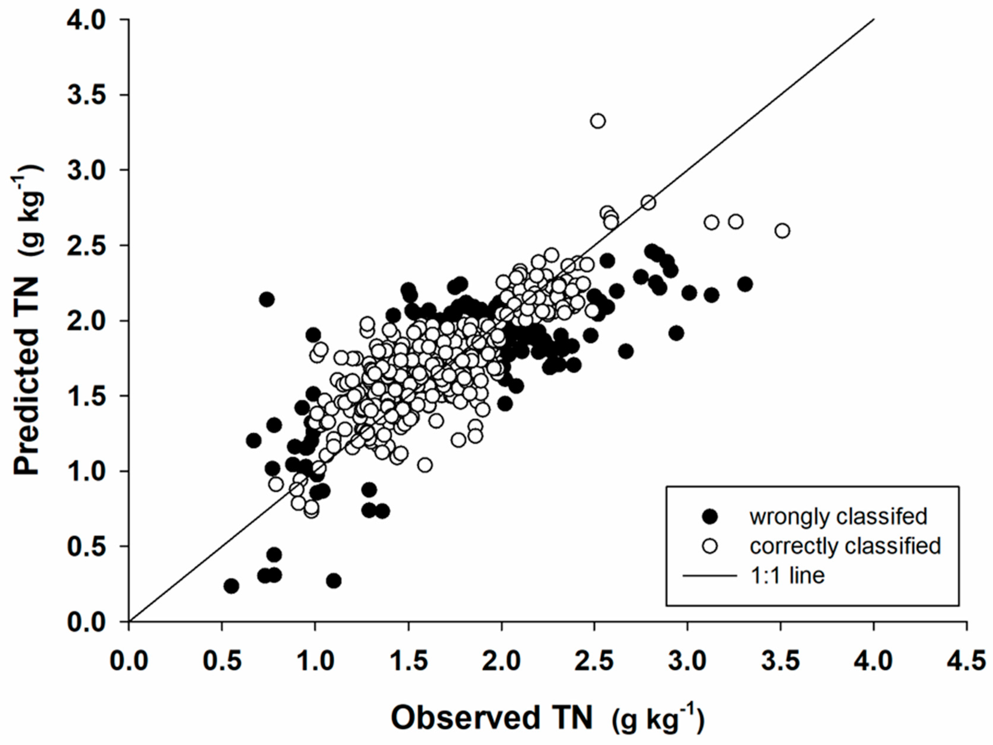
Soil Properties Predicted with High Continuous Accuracy and High Allocation Accuracy

For some soil properties (e.g., Si and TN), the predictions achieved high RPIQ and the allocations achieved high tau1. As an example, the scatterplot of the predicted versus observed TN values and the confusion matrix are presented in Figure 2 and Table 6, respectively. The RPIQ and tau1 for the estimation of TN were 2.007 and 0.709, respectively. The misclassification mostly occurred for adjacent levels (e.g., “medium” misclassified as “low” or “high”). For TN values in the range of “low” and “medium”, around 78.8% of the misallocation was caused by overestimation; while for the “high” and “extremely high” class, 100% of the misallocation was caused by underestimation.

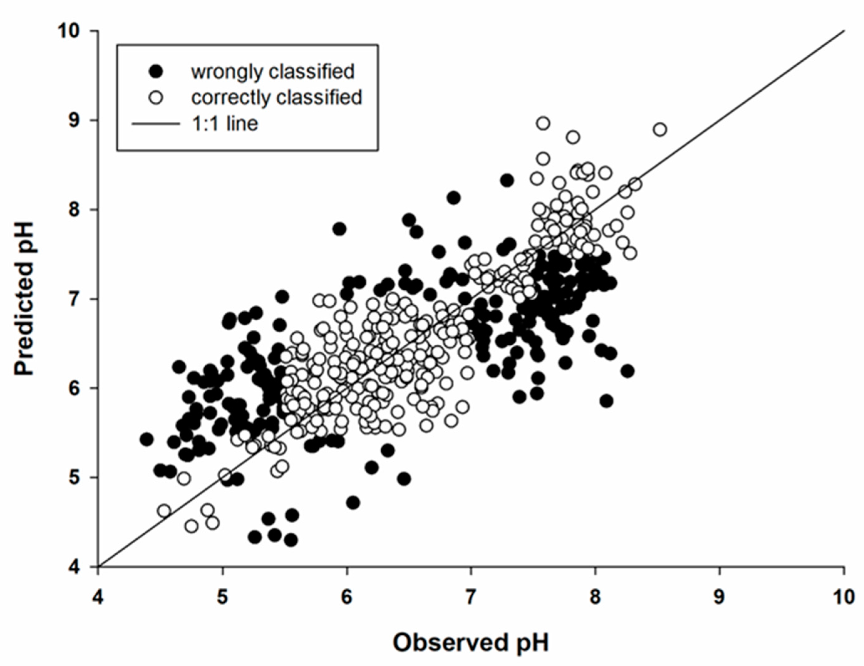
Soil Properties Predicted with Low Continuous Accuracy and High Allocation Accuracy

For another group of soil properties (e.g., Zn, Ca, Cl and Mg), the predictions achieved poor to moderate accuracy, but also achieved quite a satisfying allocation accuracy. The RPIQ of Mg (1.744) was only moderate, but it achieved the highest allocation accuracy (tau1: 0.835) compared to the other soil properties. Ca was relatively poorly predicted, with RPIQ being 1.385, but its tau1 reached 0.677. The scatterplot and confusion matrix of Ca are presented as an example for illustration (Table 7 and Figure 3). The observed values of Ca had very uneven distributions, with 78.88% of the samples falling in the class of “extremely low”.

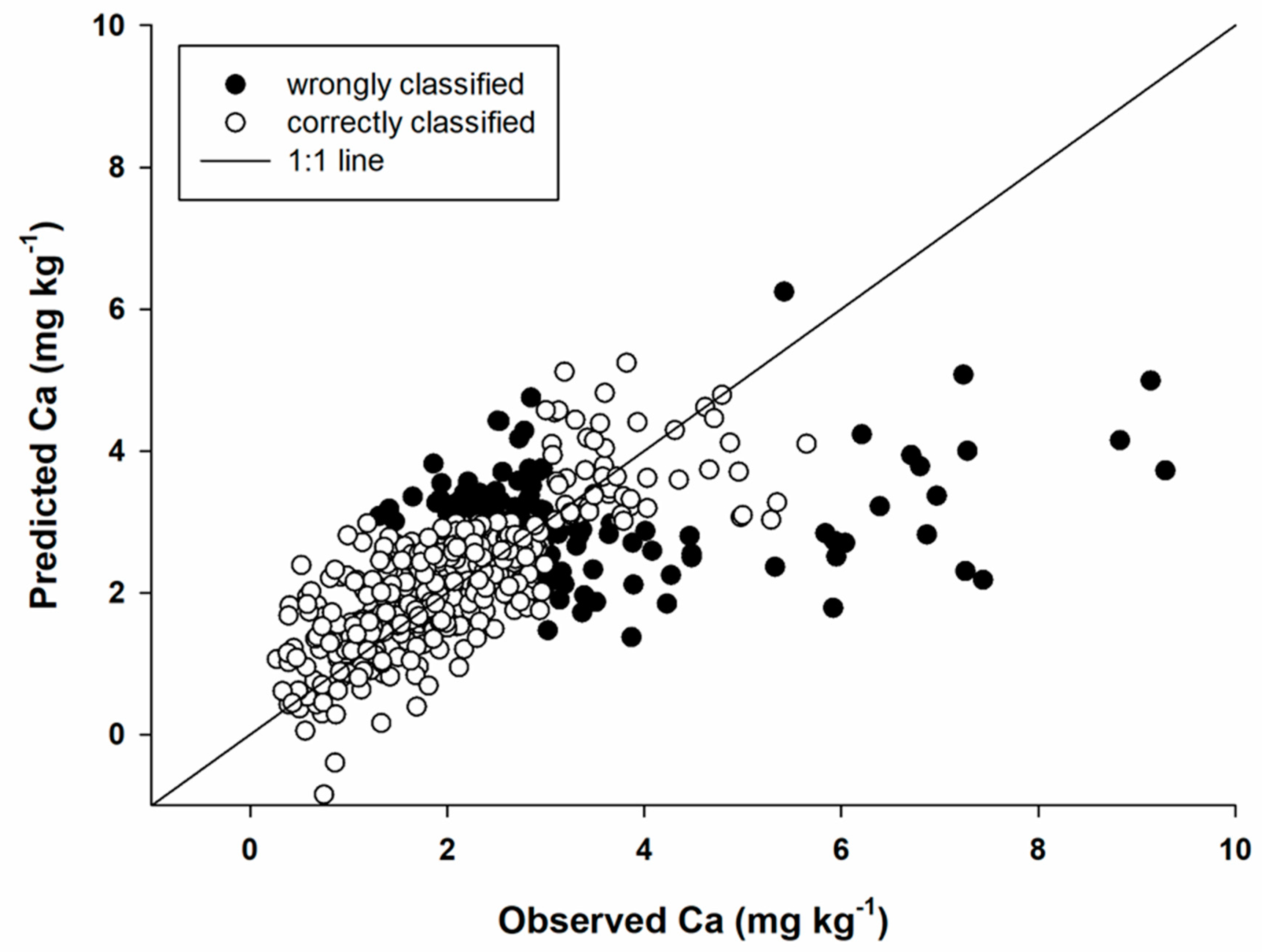
Soil properties Predicted with high Continuous Accuracy and Low Allocation Accuracy

For another group of soil properties (e.g., TK and pH) predictions achieved relatively high RPIQ, however, the allocation accuracy for these properties was relatively low. The RPIQ of pH (2.796) was the highest compared to other soil properties, but its tau1 was only 0.450 (Table 8). This can be partly explained by the relatively narrow ranges of several pH classes, e.g., the ranges for the “low” and “high” pH levels were “5.0–5.5”and “7.0–7.5”. Classification requires the predicted values to be within the specific ranges, which is quite challenging if the range is small. Among all the misclassifications, around 57.47% was misclassified as “medium”, mainly due to the fact that the “medium” class has a wide range (5.5–7.0).
Figure 4 shows the distributions of the wrongly and correctly classified points for pH on the scatterplot. Some wrongly classified points were located very close to the correctly allocated points, which indicates very similar prediction errors. The pH values of these points were close to the fertility class threshold, which was subjectively determined by stakeholders. The factor determining whether it could be correctly allocated was that if the predicted values were within or exceeding the threshold. For example, for an observed pH of 7 (high class: 7.0–7.5), if the predicted value was 6.9, it would be misclassified as “medium”, but if the predicted value was 7.1, it would be correctly classified. However, they have the same RMSE. The allocation accuracy was thus strongly influenced by the specification of user-defined thresholds.

Soil Properties Predicted with Low Continuous Accuracy and Low Allocation Accuracy

A final group of properties is represented in this study by one property, i.e., AP. This was predicted with low accuracy and poor class allocation. The RPIQ of AP was low (1.031) and its tau1 was the lowest (0.049). The low accuracy for predicting AP has also been reported by many previous researches [41], likely due to the low concentrations and the lack of direct spectral responses in the vis-NIR region (Table 9 and Figure 5).

3.3.3. Allocation Based on Three Fertility Classes

To make soil fertility management decisions, in some cases, stakeholders (e.g., farmers) do not require classification into five fertility classes for fertilization guidance. For them, three (“low”, “medium” and “high”) or even two classes (“sufficient” and “deficient”) are enough to make decisions. Table 10 compares the allocation accuracy when the soil fertility classes were reduced from five (“extremely low”, “low”, “medium”, “high” and “extremely high”) to three classes (“low”, “medium” and “high”), with “extremely low” and “low” combined as “low”, “high” and “extremely high” as “high” and “medium” as “medium”, respectively.
An increase in the allocation accuracy is to be expected due to the reduction of fertility levels and was, in fact, observed. The allocation accuracy of nine soil properties (TN, CEC, Cu, S, Zn, Si, Mn, Ca and Mg) was quite satisfactory, within the range of 0.80–1.0 (0.807–0.986). The other nine soil properties (B, TK, pH, TP, AK, AN, Fe, Mo and SOM) were allocated with acceptable accuracy, within the range of 0.60–0.80 (0.631–0.777). Only two soil properties (Cl and AP) were allocated with accuracy less than 0.60 (0.444–0.468). This shows that vis-NIR spectroscopy was fairly successful for soil fertility class allocation for most of the examined soil properties, even for some of the metals.
As evaluated by tau1, the tau1 of four soil properties (Si, Mn, Ca and Mg) were within the range of 0.8–1.0, which indicated that these four properties were classified around 80–100% better than random allocation, according to the prior probabilities; for tau1, these are equal. Twelve soil properties (pH, TP, AK, AN, Fe, Mo, SOM, TN, CEC, S, Cu and Zn) were predicted 50–80% better than random allocation on this basis, whereas Cl, AP, B and TK were less than 0.50 (0.166–0.498). However, had the classifier known the prior probabilities of the actual class distribution in the sample set, and if these fairly represent the population, the much lower values of tau2 show that the allocator’s skill would be much less.
Summarizing Table 10, the mean improvement in the overall allocation accuracy due to a reduction in the number of classes was 0.140, a substantial portion (23%) of the mean accuracy for the five-class case (0.622). This shows clearly that by reducing the number of classes required for a given fertilizer recommendation, accuracy is greatly increased.
The mean improvement for tau1 was also substantial, 0.121, which is, by coincidence, also 23% of the mean tau1 for the five-class case (0.520). This is despite the reduction in class number, which tends to decrease tau, because random allocation would be more successful with fewer classes, meaning that the mapper needs less skill to improve on that. Note also that for TN, AN, Si and Cl, tau1 did decrease, substantially for Cl.

3.4. Allocation of Soil Fertility Classes Directly from Spectra

3.4.1. Allocation Based on Five Fertility Classes

The allocation accuracy of the soil fertility classes predicted directly from spectra using the method of SVM and RF is presented in Table 11. For the evaluation of the allocation accuracy for the soil fertility classes using different models, tau1 was very consistent with the overall allocation accuracy in general, i.e., higher percentage agreement with higher tau1. However, in the direct allocation method, the classifier used an unbalanced sample set, more or less corresponding to the prior probabilities. Therefore, here, tau2 gives a better estimate of the classifier’s skill.
The allocation accuracy of SVM and RF were similar. The RF model performed slightly better than SVM for most of the properties, but for the five properties CEC, AN, AK, B and Mo, the allocation accuracy of SVM was slightly higher than that of RF. This is consistent with many studies that show that the machine learning method is much less important than the quality of the training data and the relevance to the target of the predictors (here, the spectra).
Thus, we further used the allocation results generated by RF models to compare with the indirect allocation results, i.e., to predict soil fertility indicators first by PLSR models, and then allocate these to the soil fertility class. (Table 12). The allocation accuracy of ten soil properties predicted by direct models were higher than that of the indirect models: TP, TK, AP, Ca, Fe, Mn, Cu, Zn, Mo and Cl, while the accuracy of the remaining ten soil properties based on direct models were lower than that of the indirect models. We evaluated if the allocation accuracy difference between the direct and indirect models were significant by pair-wise t-tests. No differences were statistically significant at the 5% level.
The results for tau are not comparable, because the indirect method is evaluated with tau1 and the direct method with tau2, due to the difference in prior probabilities available to the classifiers in the two cases.

3.4.2. Allocation Based on Three Fertility Classes

Table 13 shows the allocation accuracy comparison between direct and indirect models for three fertility classes. The trend was very similar to the comparison results based on five fertility classes. In this case, as in the five-class case, the overall allocation accuracy was not significantly different between the direct and indirect methods.

3.5. How much Accuracy Is Needed?

How good is good enough for soil nutrients management? There are no general answers to this question. This depends on the precision requirements from the stakeholders and the difficulty of the target soil property to be predicted. The precision requirement in turn depends on the cost of a wrong decision: extra expense if over-fertilizing, lower yield if under-fertilizing. The first is easy to determine from fertilizer prices, but the second is year-, context-, crop- and management-specific and thus would require a detailed study, where these factors are recorded or controlled.
SOM is often considered the most promising soil property which can be predicted by vis-NIR spectroscopy in replacing traditional lab analysis. However, in this study, its allocation accuracy was only moderate compared to other properties in our case. As for pH, the overall allocation accuracy for the three fertility classes was 0.677. The information of soil pH can help determine the necessity and even the quantities of lime requirements [42]. The total and available contents of N, P and K are the most common soil fertility parameters used in routine fertilization. TN and AN achieved relatively high classification accuracy, which was in accordance with previous research. The prediction of P and K was more challenging compared to N because these do not have direct spectral responses in the vis-NIR domain. However, their classification accuracy was promising, all above 0.6 (overall allocation accuracy: 0.665–0.725) except for AP. Farmers are generally more concerned about the available, rather than the total contents. The overall allocation accuracy of AN and AK was more than 0.7. Soil micronutrient management has become more and more important. Here the overall allocation accuracy was quite high. For Ca, Mg, Si, S, Mn, Cu and Z, the overall allocation accuracy ranged from 0.833 to 0.970. The overall allocation accuracy for B, Fe and Mo ranged from 0.631 to 0.765. The accuracy of Cl was the lowest (0.444). The contents of micronutrients were low and had no direct spectral response. However, their fertility classes could be predicted quite well, perhaps due to their correlations with soil properties with direct spectral responses.
In this paper we address the question: “Is reflectance spectroscopy sufficiently accurate and precise for classified soil fertility indicators?”. However, this is not a question simply about the precision of spectroscopy prediction models. It is also about the balance between the accuracy and cost, which includes the cost of the soil properties’ analysis spent; also the financial loss of “wrong fertilizer” decisions based on wrong predictions should also be considered, as explained above.
The biggest advantage of soil spectroscopy is that it is cost-effective, since it can simultaneously predict a set of soil properties, once the soil spectral library has been built. Li, Viscarra Rossel and Webster [9] have compared the cost-effectiveness of reflectance spectroscopy with the traditional dry combustion analysis for the estimation of soil organic matter. They found that the vis-NIR spectrometer on ground ≤2 mm samples proved to be the most cost-effective for soil organic carbon (SOC) estimation, considering its low cost, good accuracy and large capacity for measurements. Their study only accounted for a single property, whereas spectroscopy can be more cost-effective when used for the simultaneous estimation of a group of properties.
We made a rough comparison between the cost of the spectra measurement and soil physio-chemical properties analysis according to the lab cost standard of the Institute of Soil Science, Chinese Academy of Sciences. The cost of the soil spectral measurement is about CNY 120 per sample, including soil pre-processing, while the measurement of a set of the 20 soil properties investigated in our study costs CNY 1330 per sample. That is, the traditional cost is about eleven times more than the spectroscopy methods. In addition, there is big difference between the time costs. If the 20 soil properties of the 502 samples are measured by one laboratory technician, at least 180 workdays are needed, while the spectral measurements only require about 7 days.

3.6. Direct or Indirect Models?

In this study there was no significant difference between the allocation accuracy of the direct and indirect models for either the five- or three-class division, with the class limits from this study area. This does not agree with the results of Askari, O’Rourke and Holden [19]. In that study, predicting a soil quality index directly using spectra was superior to the indirect models, due to the accumulation of prediction errors for individual soil quality indicators. Here, however, we are predicting each property’s class separately.
So, which approach to take? The advantage of direct models is that they are concise, especially in contexts where soil properties’ data are missing or sparse in a legacy soil database, but soil fertility class information is available. The advantage of indirect models is that both specific property values and soil fertility classes can be obtained at no increase in cost except for some database manipulation. This could be useful in case some users want values (e.g., for precision agriculture) and others are satisfied with classes. The continuous property values might be more useful, considering that the classification criteria may change over time or according to different land use management.

4. Conclusions

For three fertility classes, TN, CEC, Cu, Si, Zn, S, Mn, Ca and Mg achieved a satisfying allocation accuracy of more than 0.80 (mostly above 0.85). The good allocation accuracy of micronutrients suggested that even though they are low in contents and have no direct spectral response, their correlations with other spectrally active properties can help allocate them with promising accuracy. The accuracy of pH, B, AN, TK, AK, SOM, TN, TP, Fe and Mo achieved an acceptable allocation accuracy (0.60–0.80, mostly above 0.70). Only Cl and AP were relatively poorly predicted, with an allocation accuracy of less than 0.60. The results comparing the three- and five-class divisions show that the number of classes and their ranges greatly affect user accuracy, so users should select meaningful class limits and the smallest number of classes consistent with their management skills.
Given the advantages of vis-NIR spectroscopy over standard laboratory methods, once models have been built for a recommendation domain (set of soils covering a region), spectroscopy should be considered to assist in fertilizer management. However, a comprehensive analysis of the cost-effectiveness should be investigated, considering not only the laboratory cost it saved, but also the additional cost caused by wrong fertilizer decisions based on wrong predictions. This study was only carried out in one region of one country and with just two classification levels. However, we expect similar results elsewhere and encourage service soil fertility labs to evaluate these methods.

Supplementary Materials

The following supporting information can be downloaded at: https://www.mdpi.com/article/10.3390/agronomy12081964/s1, Table S1: The soil orders in the Chinese Soil Taxonomy and their approximate WRB equivalents.

Author Contributions

Conceptualization, R.Z. and D.G.R.; formal analysis, R.Z., D.G.R. and J.Z.; investigation, K.C., W.G., W.P., Y.Z., D.L. and C.J.; writing—original draft preparation, R.Z. and D.G.R.; writing—review and editing, R.Z., D.G.R. and D.L.; supervision, D.L.; project administration, D.L.; funding acquisition, K.C. and D.L. All authors have read and agreed to the published version of the manuscript.

Funding

This research was funded by National Natural Science Foundation of China (42107322), China Tobacco Corporation Guizhou Provincial Company Science and Technology Project (201910), Natural Science Foundation of colleges and universities of Jiangsu Province (20KJB210009), and Key deployment projects of Chinese Academy of Sciences (KGFZD-135-19-10).

Institutional Review Board Statement

Not applicable.

Informed Consent Statement

Not applicable.

Data Availability Statement

Not applicable.

Conflicts of Interest

The authors declare no conflict of interest.

References

  1. Janssen, B.H.; Guiking, F.C.T.; van der Eijk, D.; Smaling, E.M.A.; Wolf, J.; van Reuler, H. A system for quantitative evaluation of the fertility of tropical soils (QUEFTS). Geoderma 1990, 46, 299–318. [Google Scholar] [CrossRef] [Green Version]
  2. D’Hose, T.; Cougnon, M.; De Vliegher, A.; Vandecasteele, B.; Viaene, N.; Cornelis, W.; Van Bockstaele, E.; Reheul, D. The positive relationship between soil quality and crop production: A case study on the effect of farm compost application. Appl. Soil Ecol. 2014, 75, 189–198. [Google Scholar] [CrossRef]
  3. Naumann, M.; Koch, M.; Thiel, H.; Gransee, A.; Pawelzik, E. The Importance of Nutrient Management for Potato Production Part II: Plant Nutrition and Tuber Quality. Potato Res. 2020, 63, 121–137. [Google Scholar] [CrossRef] [Green Version]
  4. Chen, J.; Zha, Y.; Yang, C.; Chen, T.; Xu, C.; Liu, Z.; Zhou, X. Evolution and fertilization zoning of tobacco-growing soil fertility of Shizhu county, Chongqing city. Soils 2021, 53, 1207–1214. (In Chinese) [Google Scholar]
  5. Li, Z.L.; Lu, Y.C.; Zhao, L.F.; Fan, D.S.; Wei, Z.; Zhou, W.L.; Huang, L.G.; Huang, Y.; Huang, J.P.; Gu, X.Q.; et al. Comprehensive evaluation of the suitability of tobacco planting soil fertility in Jingxi city. Crops 2021, 3, 155–160. (In Chinese) [Google Scholar]
  6. Nocita, M.; Stevens, A.; van Wesemael, B.; Aitkenhead, M.; Bachmann, M.; Barthès, B.; Ben Dor, E.; Brown, D.J.; Clairotte, M.; Csorba, A.; et al. Chapter Four—Soil Spectroscopy: An Alternative to Wet Chemistry for Soil Monitoring. In Advances in Agronomy; Sparks, D.L., Ed.; Academic Press: San Diego, CA, USA, 2015; Volume 132, pp. 139–159. [Google Scholar]
  7. Stenberg, B.; Viscarra Rossel, R.; Mouazen, A.; Wetterlind, J. Chapter Five—Visible and Near Infrared Spectroscopy in Soil Science. Adv. Agron. 2010, 107, 163–215. [Google Scholar] [CrossRef] [Green Version]
  8. Viscarra Rossel, R.A.; Behrens, T.; Ben-Dor, E.; Brown, D.J.; Demattê, J.A.M.; Shepherd, K.D.; Shi, Z.; Stenberg, B.; Stevens, A.; Adamchuk, V.; et al. A global spectral library to characterize the world’s soil. Earth-Sci. Rev. 2016, 155, 198–230. [Google Scholar] [CrossRef] [Green Version]
  9. Li, S.; Viscarra Rossel, R.A.; Webster, R. The cost-effectiveness of reflectance spectroscopy for estimating soil organic carbon. Eur. J. Soil Sci. 2022, 73, e13202. [Google Scholar] [CrossRef]
  10. Baveye, P.C.; Laba, M. Visible and near-infrared reflectance spectroscopy is of limited practical use to monitor soil contamination by heavy metals. J. Hazard. Mater. 2015, 285, 137–139. [Google Scholar] [CrossRef]
  11. Johnson, J.-M.; Vandamme, E.; Senthilkumar, K.; Sila, A.; Shepherd, K.D.; Saito, K. Near-infrared, mid-infrared or combined diffuse reflectance spectroscopy for assessing soil fertility in rice fields in sub-Saharan Africa. Geoderma 2019, 354, 113840. [Google Scholar] [CrossRef]
  12. Ji, W.; Adamchuk, V.; Chen, S.; Mat Su, A.S.; Ismail, A.; Gan, Q.; Shi, Z.; Biswas, A. Simultaneous measurement of multiple soil properties through proximal sensor data fusion: A case study. Geoderma 2019, 341, 53–69. [Google Scholar] [CrossRef]
  13. Baumann, P.; Lee, J.; Behrens, T.; Biswas, A.; Six, J.; McLachlan, G.; Viscarra Rossel, R. Modelling soil water retention and water-holding capacity with visible–near infrared spectra and machine learning. Eur. J. Soil Sci. 2022, 125, 103654. [Google Scholar] [CrossRef]
  14. De Santana, F.B.; Otani, S.K.; de Souza, A.M.; Poppi, R.J. Comparison of PLS and SVM models for soil organic matter and particle size using vis-NIR spectral libraries. Geoderma Reg. 2021, 27, e00436. [Google Scholar] [CrossRef]
  15. Ng, W.; Minasny, B.; Jones, E.; McBratney, A. To spike or to localize? Strategies to improve the prediction of local soil properties using regional spectral library. Geoderma 2022, 406, 115501. [Google Scholar] [CrossRef]
  16. Breure, T.S.; Prout, J.M.; Haefele, S.M.; Milne, A.E.; Hannam, J.A.; Moreno-Rojas, S.; Corstanje, R. Comparing the effect of different sample conditions and spectral libraries on the prediction accuracy of soil properties from near- and mid-infrared spectra at the field-scale. Soil Tillage Res. 2022, 215, 105196. [Google Scholar] [CrossRef]
  17. Chang, C.-W.; Laird, D.A.; Mausbach, M.J.; Hurburgh, C.R. Near-Infrared Reflectance Spectroscopy–Principal Components Regression Analyses of Soil Properties. Soil Sci. Soc. Am. J. 2001, 65, 480–490. [Google Scholar] [CrossRef] [Green Version]
  18. Viscarra Rossel, R.A.; Rizzo, R.; Demattê, J.A.M.; Behrens, T. Spatial Modeling of a Soil Fertility Index using Visible–Near-Infrared Spectra and Terrain Attributes. Soil Sci. Soc. Am. J. 2010, 74, 1293–1300. [Google Scholar] [CrossRef]
  19. Askari, M.S.; O’Rourke, S.M.; Holden, N.M. Evaluation of soil quality for agricultural production using visible–near-infrared spectroscopy. Geoderma 2015, 243–244, 80–91. [Google Scholar] [CrossRef]
  20. Munnaf, M.A.; Mouazen, A.M. Development of a soil fertility index using on-line Vis-NIR spectroscopy. Comput. Electron. Agric. 2021, 188, 106341. [Google Scholar] [CrossRef]
  21. Tunçay, T.; Kılıç, Ş.; Dedeoğlu, M.; Dengiz, O.; Başkan, O.; Bayramin, İ. Assessing soil fertility index based on remote sensing and gis techniques with field validation in a semiarid agricultural ecosystem. J. Arid Environ. 2021, 190, 104525. [Google Scholar] [CrossRef]
  22. Cooperative Research Group on Chinese Soil Taxonomy. Chinese Soil Taxonomy; Science Press: Beijing, China, 2001. [Google Scholar]
  23. IUSS Working Group WRB. World Reference Base for Soil Resources 2014. International Soil Classification System for Naming Soils and Creating Legends for Soil Maps; FAO: Rome, Italy, 2014. [Google Scholar]
  24. Zhang, G.-L.; Gong, Z.-T. Soil Survery Laboratory Methods; Science Press: Beijing, China, 2012. (In Chinese) [Google Scholar]
  25. Savitzky, A.; Golay, M.J.E. Smoothing and Differentiation of Data by Simplified Least Squares Procedures. Anal. Chem. 1964, 36, 1627–1639. [Google Scholar] [CrossRef]
  26. Geladi, P.; Kowalski, B.R. Partial least-squares regression: A tutorial. Anal. Chim. Acta 1986, 185, 1–17. [Google Scholar] [CrossRef]
  27. R Core Team. R: A Language and Environment for Statistical Computing; R Core Team: Vienna, Austria, 2022. [Google Scholar]
  28. Hastie, T.; Tibshirani, R.; Friedman, J. The Elements of Statistical Learning: Data Mining, Inference, and Prediction, 2nd ed.; Springer: New York, NY, USA, 2009. [Google Scholar]
  29. Brungard, C.W.; Boettinger, J.L.; Duniway, M.C.; Wills, S.A.; Edwards, T.C. Machine learning for predicting soil classes in three semi-arid landscapes. Geoderma 2015, 239–240, 68–83. [Google Scholar] [CrossRef] [Green Version]
  30. Chen, S.; Li, S.; Ma, W.; Ji, W.; Xu, D.; Shi, Z.; Zhang, G. Rapid determination of soil classes in soil profiles using vis–NIR spectroscopy and multiple objectives mixed support vector classification. Eur. J. Soil Sci. 2019, 70, 42–53. [Google Scholar] [CrossRef] [Green Version]
  31. Chen, J.; Tang, Y.J. Analysis on soil fertility of main district planting flue-cured tobacco in Guizhou. Chin. Agric. Sci. Bull. 2006, 22, 356–359. (In Chinese) [Google Scholar]
  32. Congalton, R.; Green, K. Assessing the Accuracy of Remotely Sensed Data: Principles and Practices, 3rd ed.; CRC Press: Boca Raton, FL, USA, 2019. [Google Scholar]
  33. Ma, Z.; Redmond, R. Tau Goetficients for Accuracy Assessment of Classificationf Remote Sensing Data. Photogramm. Eng. Remote Sens. 1995, 61, 435–439. [Google Scholar]
  34. Pontius, R.G.; Millones, M. Death to Kappa: Birth of quantity disagreement and allocation disagreement for accuracy assessment. Int. J. Remote Sens. 2011, 32, 4407–4429. [Google Scholar] [CrossRef]
  35. Rossiter, D.G.; Zeng, R.; Zhang, G.-L. Accounting for taxonomic distance in accuracy assessment of soil class predictions. Geoderma 2017, 292, 118–127. [Google Scholar] [CrossRef] [Green Version]
  36. Beaudette, D.; Roudier, P.; Brown, A. Algorithms for Quantitative Pedology. R Package, Version 1.29. 2022. Available online: https://github.com/ncss-tech/aqp (accessed on 1 July 2022).
  37. Beaudette, D.E.; Roudier, P.; O’Geen, A.T. Algorithms for quantitative pedology: A toolkit for soil scientists. Comput. Geosci. 2013, 52, 258–268. [Google Scholar] [CrossRef]
  38. Awiti, A.O.; Walsh, M.G.; Shepherd, K.D.; Kinyamario, J. Soil condition classification using infrared spectroscopy: A proposition for assessment of soil condition along a tropical forest-cropland chronosequence. Geoderma 2008, 143, 73–84. [Google Scholar] [CrossRef]
  39. Soriano-Disla, J.M.; Janik, L.J.; Viscarra Rossel, R.A.; Macdonald, L.M.; McLaughlin, M.J. The Performance of Visible, Near-, and Mid-Infrared Reflectance Spectroscopy for Prediction of Soil Physical, Chemical, and Biological Properties. Appl. Spectrosc. Rev. 2014, 49, 139–186. [Google Scholar] [CrossRef]
  40. Mouazen, A.M.; Kuang, B.; De Baerdemaeker, J.; Ramon, H. Comparison among principal component, partial least squares and back propagation neural network analyses for accuracy of measurement of selected soil properties with visible and near infrared spectroscopy. Geoderma 2010, 158, 23–31. [Google Scholar] [CrossRef]
  41. Ng, W.; Husnain; Anggria, L.; Siregar, A.F.; Hartatik, W.; Sulaeman, Y.; Jones, E.; Minasny, B. Developing a soil spectral library using a low-cost NIR spectrometer for precision fertilization in Indonesia. Geoderma Reg. 2020, 22, e00319. [Google Scholar] [CrossRef]
  42. Viscarra Rossel, R.; Walvoort, D.J.J.; McBratney, A.; Janik, L.; Skjemstad, J.O. Proximal sensing of soil pH and lime requirement by mid infrared diffuse reflectance spectroscopy. In 3 ECPA-EFITA Proceedings, Proceedings of the Third European Conference on Precision Agriculture, Montpellier, France, 1 January 2001; pp. 497–502; Grenier, G., Blackmore, S., Steffe., J., Eds.; Agro Montpellier: Montepellier, France, 2001. [Google Scholar]
Figure 1. Distribution of sampling points.
Agronomy 12 01964 g001
Figure 2. Scatterplot of the predicted TN values versus the observed TN values.
Agronomy 12 01964 g002
Figure 3. Scatterplot of the predicted Ca values versus the observed Ca values.
Agronomy 12 01964 g003
Figure 4. Scatterplot of the predicted pH values versus the observed pH values.
Agronomy 12 01964 g004
Figure 5. Scatterplot of the predicted AP values versus the observed AP values.
Agronomy 12 01964 g005
Table 1. Criteria of fertility classes for different soil properties.
Fertility Indicators Extremely LowLowMediumHighExtremely High
pH<5.05.0~5.55.5~7.07.0~7.5≥7.5
SOM (g kg−1)<1010~1515~3030~40≥40
TN (g kg−1)<0.50.5~11~22~2.5≥2.5
CEC (cmol(+) kg−1)<6.26.2–10.510.5–15.415.4–20.0≥20
TP (g kg−1)<0.50.5~11~1.5≥1.5/
TK (g kg−1)<1010~1515~2020~25≥25
AN (mg kg−1)<6565~100100~180180~240≥240
AP (mg kg−1)<1010~1515~3030~40≥40
AK (mg kg−1)<8080~150150~220220~350≥350
Ca (cmol(1/2Ca2+) kg−1)<33~66~1010~18≥18
Mg (cmol(1/2Mg2+) kg−1)<0.50.5~1.01.0~1.61.6~3.2≥3.2
Si (mg kg−1)<5050~100100~150≥150/
S (mg kg−1)<1010~1616~3030~50≥50
B (mg kg−1)<0.150.15~0.30.3~0.60.6~1.0≥1.0
Fe (mg kg−1)<2.52.5~4.54.5~1010~60≥60
Mn (mg kg−1)<55~1010~2020~40≥40
Cu (mg kg−1)<0.20.2~0.50.5~1.01.0~3.0≥3.0
Zn (mg kg−1)<0.50.5~1.01.0~2.02.0~4.0≥4.0
Mo (mg kg−1)<0.10.1~0.150.15~0.20.2~0.3≥0.3
Cl (mg kg−1)<55~1010~3030~40≥40
Soil organic matter (SOM), total nitrogen (TN), total phosphorus (TP), total potassium (TK), alkali-hydrolyzable nitrogen (AN), available phosphorus (AP), available potassium (AK), available calcium (Ca), available magnesium (Mg), available silicon (Si), available sulfur (S), available boron (B), available iron (Fe), available manganese (Mn), available copper (Cu), available zinc (Zn), available molybdenum (Mo) and available chlorine (Cl).
Table 2. Statistical summary of the 20 soil fertility indicators.
Fertility IndicatorsMin1st QuartileMedian3rd QuartileMaxCoefficient
of Variation (%)
KurtosisSkewness
pH4.395.646.487.5058.5215.59%−1.19−0.07
SOM (g kg−1)5.9624.2029.7635.9389.6431.73%1.090.62
CEC (cmol(+) kg−1)6.2715.2218.5121.9735.3226.75%0.350.48
TN (g kg−1)0.551.431.682.033.5126.63%0.590.48
TP (g kg−1)0.110.680.831.0210.7362.29%184.9711.11
TK (g kg−1)2.179.0413.6519.6841.3750.44%−0.120.62
AN (mg kg−1)0.01124.95143.33176.40316.0527.50%1.080.57
AP (mg kg−1)0.2616.6325.4242.60251.8179.41%15.422.80
AK (mg kg−1)40.00210.00312.50450.001480.0054.37%2.931.22
Ca (cmol(1/2Ca2+) kg−1)1.331.402.132.8646.4358.29%4.801.74
Mg (cmol(1/2Mg2+) kg−1)0.100.120.210.425.4880.87%0.861.25
Si (mg kg−1)52.38189.65283.31390.03756.7644.85%−0.300.52
S (mg kg−1)1.2539.2669.83125.21469.6577.28%4.401.77
B (mg kg−1)0.110.410.681.295.7184.43%5.642.08
Fe (mg kg−1)0.099.2231.8752.33230.2098.11%4.761.91
Mn (mg kg−1)2.1370.85110.03129.79169.1041.76%−0.49−0.71
Cu (mg kg−1)0.051.582.864.0318.2473.87%9.202.19
Zn (mg kg−1)0.194.277.209.9675.3092.44%24.773.94
Mo (mg kg−1)0.020.200.320.472.6080.66%13.443.08
Cl (mg kg−1)07.1014.2021.30390.50135.49%95.207.84
Table 3. Summary statistics of soil fertility classes.
Fertility IndicatorsExtremely LowLowMediumHighExtremely High
Range Range Range Range Range
pH<5.06.77%5.0~5.513.55%5.5~7.042.83%7.0~7.511.75%≥7.525.10%
SOM (g kg−1)<100.80%10~153.19%15~3046.81%30~4033.46%≥4015.74%
CEC (cmol(+) kg−1)<6.20.00%6.2~10.53.19%10.5~15.423.31%15.4~2036.45%≥2037.05%
TN (g kg−1)<0.50.00%0.5~15.18%1~267.73%2~2.521.91%≥2.55.18%
TP (g kg−1)<0.58.57%0.5~164.54%1~1.521.51%≥1.55.38%//
TK (g kg−1)<1030.48%10~1525.70%15~2019.92%20~2512.75%≥2511.15%
AN (mg kg−1)<650.80%65~1008.77%100~18066.53%180~24021.51%≥2402.39%
AP (mg kg−1)<1011.75%10~1510.56%15~3037.25%30~4012.75%≥4027.69%
AK (mg kg−1)<802.79%80~1508.76%150~22015.34%220~35030.08%≥35043.03%
Ca (cmol(1/2Ca2+) kg−1)<378.88%3~618.33%6~102.79%10~180.00%≥180.00%
Mg (cmol(1/2Mg2+) kg−1)<0.578.49%0.5~1.020.12%1.0~1.61.39%1.6~3.20.00%≥3.20.00%
Si (mg kg−1)<500.00%50~1002.79%100~15011.15%≥15086.06%//
S (mg kg−1)<100.60%10~161.20%16~3011.35%30~5022.71%≥5064.14%
B (mg kg−1)<0.151.20%0.15~0.39.96%0.3~0.631.87%0.6~1.023.11%≥1.033.86%
Fe (mg kg−1)<2.58.17%2.5~4.57.97%4.5~109.36%10~6055.98%≥6018.52%
Mn (mg kg−1)<50.60%5~102.39%10~204.38%20~405.58%≥4087.05%
Cu (mg kg−1)<0.21.79%0.2~0.54.58%0.5~1.011.16%1.0~3.036.45%≥3.046.02%
Zn (mg kg−1)<0.52.39%0.5~1.08.17%1.0~2.04.78%2.0~4.08.17%≥4.076.49%
Mo (mg kg−1)<0.15.78%0.1~0.157.57%0.15~0.211.35%0.2~0.319.52%≥0.355.78%
Cl (mg kg−1)<57.57%5~1034.27%10~3044.22%30~404.38%≥409.56%
For each fertility class, the left column indicates the specific ranges while the right column indicates the corresponding proportion. “/” indicates that there is no such class for this property.
Table 4. Prediction accuracy of soil fertility indicators by PLSR models.
Soil Fertility IndicatorsR2RMSERPIQ
pH0.5710.6672.796
SOM (g kg−1)0.5996.4041.832
CEC (cmol(+) kg−1)0.6263.0792.192
TN (g kg−1)0.5880.2992.007
TP (g kg−1)0.1090.5330.638
TK (g kg−1)0.5594.9622.144
AN (mg kg−1)0.46132.1441.601
AP (mg kg−1)0.03725.1911.031
AK (mg kg−1)0.058184.3211.302
Ca (cmol(1/2Ca2+) kg−1)0.4031.0541.385
Mg (cmol(1/2Mg2+) kg−1)0.5180.1721.744
Si (mg kg−1)0.57187.3012.295
S (mg kg−1)0.19664.3151.336
B (mg kg−1)0.1980.7411.188
Fe (mg kg−1)0.36130.9411.393
Mn (mg kg−1)0.28834.8321.692
Cu (mg kg−1)0.3321.8831.301
Zn (mg kg−1)0.0467.4300.765
Mo (mg kg−1)0.1710.2810.961
Cl (mg kg−1)0.01226.1720.543
Table 5. Allocation accuracy of individual soil fertility class based on predictions from PLSR models (five fertility classes).
Fertility IndicatorsOverall Allocation
Accuracy
tau1tau2
pH0.5600.4500.233
SOM (g kg−1)0.6630.5790.455
CEC (cmol(+) kg−1)0.6510.5350.463
TN (g kg−1)0.7670.7090.432
TP (g kg−1)0.6120.4820.172
TK (g kg−1)0.4660.3330.278
AN (mg kg−1)0.7030.6290.158
AP (mg kg−1)0.2390.049−0.533
AK (mg kg−1)0.4140.0490.154
Ca (cmol(1/2Ca2+) kg−1)0.7850.6770.417
Mg (cmol(1/2Mg2+) kg−1)0.8760.8350.550
Si (mg kg−1)0.8630.8170.267
S (mg kg−1)0.6410.552−0.306
B (mg kg−1)0.4300.2880.142
Fe (mg kg−1)0.5840.4800.180
Mn (mg kg−1)0.8670.833−1.016
Cu (mg kg−1)0.5480.4350.190
Zn (mg kg−1)0.7630.4350.405
Mo (mg kg−1)0.5560.445−0.182
Cl (mg kg−1)0.4440.4450.171
tau1 is the tau index calculated based on equal prior probability, while tau2 is based on the prior probability of the reference set, highest values per evaluation statistic are in bold.
Table 6. Allocation confusion matrix of TN.
ObservedExtremely LowLowMediumHighExtremely HighUser’s Accuracy
Predicted
Extremely low041000.00%
Low0660050.00%
Medium01530746282.97%
High0126641659.81%
Extremely high00008100.00%
Table 7. Allocation confusion matrix of Ca.
ObservedExtremely LowLowMediumHighExtremely HighUser’s Accuracy
Predicted
Extremely low3393740089.21%
Low5655100045.45%
Medium010000.00%
High00000100.00%
Extremely high00000100.00%
Table 8. Allocation confusion matrix of pH.
ObservedExtremely LowLowMediumHighExtremely HighUser’s Accuracy
Predicted
Extremely low6550037.50%
Low101270041.38%
Medium1850181273258.77%
High0116294133.33%
Extremely high00635385.48%
Table 9. Allocation confusion matrix of AP.
ObservedExtremely LowLowMediumHighExtremely HighUser’s Accuracy
Predicted
Extremely low10000100.00%
Low2210133.33%
Medium222066191945.21%
High33291084311113.27%
Extremely high12122832.00%
Table 10. Comparison of the allocation accuracy for five fertility classes versus three fertility classes.
Soil PropertiesFive Fertility ClassesThree Fertility Classes
Overall Allocation
Accuracy
tau1tau2Overall Allocation
Accuracy
tau1tau2
pH0.5600.4500.2330.6770.5160.388
SOM0.6630.5790.4550.7770.6650.571
CEC0.6510.5350.4630.8190.7280.478
TN0.7670.7090.4320.8070.7070.516
TP0.6120.4820.1720.6950.5430.271
TK0.4660.3330.2780.6650.4980.446
AN0.7030.6290.1580.7350.6030.243
AP0.2390.049−0.5330.4680.202−0.232
AK0.4140.2680.1540.7250.588−6.775
Ca0.7850.6770.4170.9700.940−6.515
Mg0.8760.8350.5500.9860.979−0.755
Si0.8630.8170.2670.8710.8060.308
S0.6410.552−0.3060.8330.749−0.626
B0.4300.2880.1420.6310.447−0.030
Fe0.5840.4800.1800.7590.638−0.064
Mn0.8670.833−1.0160.9220.883−1.199
Cu0.5480.4350.1900.8330.749−0.378
Zn0.7630.7040.4050.8490.773−18.057
Mo0.5560.445−0.1820.7650.647−0.607
Cl0.4440.3050.1710.4440.1660.089
Five fertility classes: extremely low, low, medium, high and extremely high. Three fertility classes: low, medium and high, “extremely low” and “low” combined as “low”, “high” and “extremely high” as “high” and medium as “medium”, highest values per evaluation statistic are in bold.
Table 11. Allocation accuracy of soil fertility classes directly from spectra (five fertility classes).
Soil PropertiesSVMRF
Overall Allocation
Accuracy
tau1tau2Overall Allocation
Accuracy
tau1tau2
pH0.4720.3400.2640.4960.3700.297
SOM0.5700.4620.3310.5900.4870.362
CEC0.6320.5390.4530.6120.5140.424
TN0.6810.6020.1740.6870.6090.359
TP0.6410.5520.2920.6630.5760.328
TK0.4000.2510.2240.4680.3350.312
AN0.6630.5790.3300.6470.5590.299
AP0.4140.2680.2120.4260.2830.228
AK0.4280.2850.1740.4140.2680.154
Ca0.7830.7290.3720.7910.7390.395
Mg0.7790.7240.3640.8290.7860.508
Si0.7090.6370.3690.7190.6490.391
S0.6410.5520.3160.6410.5520.316
B0.4080.2610.1770.3940.2430.158
Fe0.5600.4500.3020.6260.5320.406
Mn0.8710.8380.4530.8750.8430.470
Cu0.4860.3580.1980.5680.4600.325
Zn0.7650.7060.4100.7830.7290.455
Mo0.5620.4520.2960.5600.4500.292
Cl0.4460.3080.1740.4640.3310.201
SVM: Support Vector Machine, RF: Random Forest; tau1: tau calculated based on equal prior probability; tau2: tau calculated based on the probability of the reference set, highest values per evaluation statistic are in bold.
Table 12. Comparison between direct allocation and indirect allocation (five fertility classes).
Soil PropertiesIndirect AllocationDirect Allocation (RF)
Overall Allocation
Accuracy
tau1tau2Overall Allocation
Accuracy
tau1tau2
pH0.5600.4500.2330.4960.3700.297
SOM0.6630.5790.4550.5900.4870.362
CEC0.6510.5350.4630.6120.5140.424
TN0.7670.7090.4320.6870.6090.359
TP0.6120.4820.1720.6630.5760.328
TK0.4660.3330.2780.4680.3350.312
AN0.7030.6290.1580.6470.5590.299
AP0.2390.049−0.5330.4260.2830.228
AK0.4140.2680.1540.4140.2680.154
Ca0.7850.6770.4170.7910.7390.395
Mg0.8760.8350.5500.8290.7860.508
Si0.8630.8170.2670.7190.6490.391
S0.6410.552−0.3060.6410.5520.316
B0.4300.2880.1420.3940.2430.158
Fe0.5840.4800.1800.6260.5320.406
Mn0.8670.833−1.0160.8750.8430.470
Cu0.5480.4350.1900.5680.4600.325
Zn0.7630.7040.4050.7830.7290.455
Mo0.5560.445−0.1820.5600.4500.292
Cl0.4440.3050.1710.4640.3310.201
RF: Random Forest; tau1: tau calculated based on equal prior probability; tau2: tau calculated based on the probability of the reference set, highest values per evaluation statistic are in bold.
Table 13. Comparison between direct allocation and indirect allocation (three fertility classes).
Soil PropertiesIndirect AllocationDirect Allocation
Overall Allocation
Accuracy
tau1tau2Overall Allocation
Accuracy
tau1tau2
pH0.6770.5160.3880.5380.3070.277
SOM0.7770.6650.5710.7350.6210.507
CEC0.8190.7280.4780.8050.7070.517
TN0.8070.7070.5160.7410.6120.443
TP0.6950.5430.2710.7490.6240.375
TK0.6650.4980.4460.6850.5280.464
AN0.7350.6030.2430.6650.4980.319
AP0.4680.202−0.2320.5000.2500.228
AK0.7250.588−6.7750.7170.5760.340
Ca0.9700.940−6.5150.9720.9580.486
Mg0.9860.979−0.7550.9860.9790.493
Si0.8710.8060.3080.8630.7940.442
S0.8330.749−0.6260.8650.7970.417
B0.6310.447−0.0300.6000.3990.282
Fe0.7590.638−0.0640.7810.6710.466
Mn0.9220.883−1.1990.9220.8840.442
Cu0.8330.749−0.3780.8450.7670.488
Zn0.8490.773−18.0570.8630.7940.491
Mo0.7650.647−0.6070.7850.6770.437
Cl0.4440.1660.0890.4880.2320.161
tau1: tau calculated based on equal prior probability; tau2: tau calculated based on the probability of the reference set, highest values per evaluation statistic are in bold.
Publisher’s Note: MDPI stays neutral with regard to jurisdictional claims in published maps and institutional affiliations.

