Abstract
As we know, climate change and climate variability significantly influence the most important component of global hydrological cycle, i.e., rainfall. The study pertaining to change in the spatio-temporal patterns of rainfall dynamics is crucial to take appropriate actions for managing the water resources at regional level and to prepare for extreme events such as floods and droughts. Therefore, our study has investigated the spatio-temporal distribution and performance of seasonal rainfall for all districts of Haryana, India. The gridded rainfall datasets of 120 years (1901 to 2020) from the India Meteorological Department (IMD) were categorically analysed and examined with statistical results using mean rainfall, rainfall deviation, moving-average, rainfall categorization, rainfall trend, correlation analysis, probability distribution function, and climatology of heavy rainfall events. During each season, the eastern districts of Haryana have received more rainfall than those in its western equivalent. Rainfall deviation has been positive during the pre-monsoon season, while it has been negative for all remaining seasons during the third quad-decadal time (QDT3, covering the period of 1981–2020); rainfall has been declining in most of Haryana’s districts during the winter, summer monsoon, and post-monsoon seasons in recent years. The Innovative Trend Analysis (ITA) shows a declining trend in rainfall during the winter, post-monsoon, and summer monsoon seasons while an increasing trend occurs during the pre-monsoon season. Heavy rainfall events (HREs) were identified for each season from the last QDT3 (1981–2020) based on the available data and their analysis was done using European Centre for Medium-Range Weather Forecasts (ECMWF) reanalysis Interim (ERA-Interim), which helped in understanding the dynamics of atmospheric parameters during HREs. Our findings are highlighting the qualitative and quantitative aspects of seasonal rainfall dynamics at the districts level in Haryana state. This study is beneficial in understanding the impact of climate change and climate variability on rainfall dynamics in Haryana, which may further guide the policymakers and beneficiaries for optimizing the use of hydrological resources.
1. Introduction
Climate change and climate variability directly affect the rainfall dynamics in different parts of the world [1,2,3]. There has always been a challenge to identify and quantify the impact of climate change as it is influenced by the local factors [4]. Several scientists across the globe have studied the impact of climate change using various climatic indices [5,6,7,8]. These climate change studies are conducted by analyzing the trends present in the long-term meteorological data, mainly related with rainfall and temperature. Several studies have reported decline in rainfall and increase in frequency of droughts due to continuous rise in global temperature resulting from climate change [9,10,11]. Climate change and climate variability results in the increased occurrence of extreme weather events such as heat and cold waves, floods, and droughts, which severely affects human and animal health, environment, and socio-economic conditions [12]. Climate change significantly alters the rainfall amount and distribution [13,14,15], which requires urgent consideration and systematic research. Since rainfall is such an important part of the hydrological cycle, it’s crucial to look into noticeable climate changes, especially the vicissitudes in rainfall intensity and distribution patterns, in climatological, hydrological, meteorological, industrial, and agricultural studies around the world for a sustainable allocation of water resources, which necessitates a thorough understanding of long-term rainfall dynamics.
Haryana is popularly known as the breadbasket of India as it provides significant amounts of paddy during kharif season and wheat during rabi season [16,17], but currently the agriculture in Haryana is facing problems related to lower availability of irrigation water and higher costs of pumping the groundwater. As Haryana is one of the major states producing paddy in the country [18,19,20], the increased pumping of groundwater for paddy cultivation has resulted in severe decline in its level [21,22]. Due to these alarming circumstances, it is critical to monitor Haryana’s water supplies by recognizing shifting rainfall patterns in order to properly and timely allocate funds or necessary inputs, prepare for adverse weather events such as droughts and floods, and sustainably manage water resources throughout the year. Rainfall has an impact on agricultural production by influencing soil moisture and availability to crops, as well as soil health by causing soil erosion, land degradation, and desertification, as well as the region’s power generation and industrial output, all of which have an impact on the state’s overall economy.
Rainfall studies at the regional level are critical because they aid in anticipating difficulties that influence the region’s natural resources and economic activity. Rainfall trends over time are a proxy for climate change. The spatio-temporal trends in rainfall must be discovered and embraced as signals of climate change at the regional level. Heavy rainfall exacerbates floods, while droughts are caused by insufficient rainfall, resulting in lower agricultural production. Various numerical modelling studies imply that rising CO2 concentrations are strongly linked to an increase in the frequency of extreme events with inter-annual variability in rainfall. The trend analysis of historical rainfall data provides insight into regional rainfall characteristics and aids policymakers in developing efficient hydrological policies to combat drought and reduce flood risk through adequate water resource management. Therefore, we used innovative trend analysis (ITA) in this study, which is a novel and rigorous approach of trend detection and has been successfully applied to quantify trends in hydro-meteorological variables in a variety of studies such as rainfall [23,24,25], temperature [26], drought variables [27], evapotranspiration [28], and water quality parameters [29,30] all throughout the world. However, there have been no previous studies that have employed ITA to find trends in a century-long rainfall series in Haryana.
Several academics have investigated the rainfall dynamics in various geographical places throughout the world [31,32,33,34]. With relation to climate change and extreme rainfall events in India, a number of researchers have investigated the spatio-temporal dynamics of rainfall and its amplitude in hydrological and meteorological time series datasets on a regional and nationwide level [35,36,37,38]. Patra et al. [39] found a non-significant drop in monsoonal and annual rainfall for Odisha state over time, but an increase in post-monsoonal rainfall. Kerala’s long-term rainfall data was investigated by Krishnakumar et al. [40], who discovered a significant decrease in southwest monsoonal season rainfall and an increase in post-monsoonal season rainfall. Seasonal heavy rainfall events have become more common in India in recent years, causing significant harm to human life and property. During the monsoon season, Mumbai floods [41,42] occurred in 2005, Uttarakhand floods [43,44,45] occurred in 2013, and Kerala floods [46,47] occurred in 2018, respectively, whilst Chennai floods [48,49,50,51] occurred during the post-monsoon season in 2015. All of these extreme weather events have occurred in recent decades owing to climate change, resulting in significant casualties and losses. From 1910 to 2000, Sen and Balling [52] discovered a rise in the occurrence of extreme events in India. In Central India, Goswami et al. [53] found a significant increase in the quantity and frequency of heavy monsoonal rainfall. Rajeevan et al. [54] found a drop in moderate rainfall events, with considerable variability in the frequency of severe rainfall events at the inter-decade and inter-annual time scales, which led to large risks of catastrophic floods in central India, which were consistent with Goswami et al. [53]. In the second half of the twentieth century, Vittal et al. [55] reported a rise in spatially aggregated extreme rainfall events throughout India; nevertheless, significant differences in the pattern of extremes events were also observed during the pre- and post-1950 eras.
The reason for using the district as an administrative unit in this study is to represent the spatio-temporal patterns of seasonal rainfall, which is one of the major constraints to agricultural and other socio-economic activity in many parts of Haryana. However, only a few district-level analyses focusing on spatio-temporal dynamics of seasonal rainfall have been carried out across the state. This research is needed to gain a better knowledge of rainfall dynamics, which will aid in assessing the changing rainfall pattern over the study period and detecting hotspots where the frequency of above and below normal rainfall is increasing. This could aid policymakers in locating possible drought and flood-prone areas at the micro-level, allowing them to better manage available resources and make timely socio-economic decisions across the state. Furthermore, the district-level rainfall datasets employed in this analysis span more than a century, which is a significant improvement above previous Haryana studies. The goal of the current study is to analyse the distribution pattern and trends of seasonal rainfall data for all 22 districts of Haryana, India, during a period of 120 years (1901–2020). There are five sections to this study. The data used and the study region are described in Section 2. Section 3 and Section 4 deal with methodology, outcomes, and discussions, respectively. The study’s conclusions are stated in Section 5.
2. Study Area and Data
The study area comprises 22 districts of Haryana, as shown in Figure 1. Haryana is situated in north-west region of India and covers about 1.3% area of the country. The location of the study area extends from 27°39′ to 30°35′ N and 74°28′ to 77°36′ E, respectively, with a geographical area of about 44,212 km2 and altitude ranging from 100 m to 1500 m and with a mean altitude of 238 m above mean sea level. Among districts, PK has the highest mean elevation of 506 m, whereas the lowest mean elevation of 192 m is of PL. The climate of Haryana state is subtropical, semi-arid to sub-humid, continental, and monsoon type with mean annual rainfall ranging from 500 to 1000 mm and more than 75% of it is received between June and September [56]. Remaining 10–15%, 5–10%, and 5–10% rains are fallen in winter, summer and post monsoon season, respectively. There is a great change in temperatures in the area and the hottest months are May and June while the January and February are the coldest. Maximum temperature in the area exceeds 40 °C in May and June and hot dry winds are commonly observed. Average temperature in the region varies from 6 to 8 °C and frost may be observed in one or two days in the winter season.
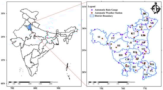
Figure 1.
Location map of study area showing the network location of automatic weather stations and rain gauges of India Meteorological Department in the different districts of Haryana.
In the present study, daily rainfall data covering a period of 1901–2020 (120 years) provided by the India Meteorological Department (IMD) at a grid resolution of 0.25 × 0.25 degree, was directly projected on the district shapefile of Haryana state and the zonal-statistical average of the bound district region was processed and used for the analysis. This high-resolution gridded dataset was developed using daily rainfall data records collected from a network of 6955 rain gauge stations over India by Pai et al. [57]. The European Centre for Medium-Range Weather Forecasts (ECMWF) reanalysis Interim (ERA-Interim), a very high spatial resolution data of 0.125 × 0.125 degree with 60 vertical levels starting right from the surface up to 0.1 hPa top-level, which is available on daily basis from 1979 to present [58,59]; hereafter referred to as ERA, was used to study the climatology of heavy rainfall events. ERA covers the global atmospheric parameters such as zonal and meridional circulation and specific humidity at various pressure levels.
3. Methods
Urbanization in India started to intensify post-independence in 1947 [60]. The Green Revolution in India was initiated in the 1960s, which refers to a period when agriculture was converted into an industrial system due to the adoption of modern methods and technology, such as the introduction of high yielding variety (HYV) seeds, tractors, irrigation facilities, pesticides, and fertilizers to increase food production in order to alleviate hunger and poverty. Following a clear shift towards economic liberalisation in the 1980s, Indian economy has grown remarkably because of increased industrialization [61], but high-intensity agriculture during the green revolution was heavily dependent on pesticides and chemical fertilizers, especially those containing nitrogen. Since 1960, the worldwide rate of application of nitrogen fertilizers has increased by several times [62,63]. Such rapid urbanization, industrialization, and intensive agricultural activities since the green revolution are attributed as the main reason for changing the rainfall pattern and extreme events. Haryana served as epicentre of green revolution in India [64,65]. Based on this background, we sliced the period of 120 years into 3 quad-decadal times (QDT) intervals of 40 years each, viz: QDT1, QDT2, and QDT3 for analysing rainfall dynamics where QDT1 corresponds to pre-urbanization era (1901–1940), QDT2 corresponds to accelerated industrialization, urbanization, and green revolution era (1941–1980), and QDT3 corresponds to recent climate (1981–2020).
IMD has meteorologically defined four seasons over India which are, viz: winter (January–February), pre-monsoon (March–May), summer monsoon (June–September), and post-monsoon (October–December). The total seasonal data for each season was calculated by cumulating the daily data of each district. Basic statistical analysis including mean, per cent deviation of rainfall (PDR), correlation coefficient (CC), trend detection with ITA, moving average for seasonal rainfall were implemented for comparison and visualization of the time series data (Figure 2).
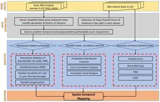
Figure 2.
The schematic flow chart of the methodology.
3.1. Distribution Pattern of Rainfall
The normal seasonal rainfall for each district was computed as Mean Rainfall (MR) by taking the average of rainfall for the whole study period of 120 years. Similarly, MR for each season rainfall of all the districts was calculated for QDT1, QDT2, and QDT3.
The seasonal rainfall deviation at a district during each QDT was calculated by expressing the monsoon rainfall in terms of the per cent departure from its long term climatological mean value of 120 years and is termed as Percent Deviation of Rainfall (PDR). Positive PDR points toward above normal, while negative PDR depicts Below Normal Rainfall (BNR), during that specific QDT.
where RQDT is the seasonal rainfall of the district during any QDT, is the climatological long term mean rainfall of 120 (1901–2020) years referred as CLM120 hereafter.
Inter-annual variability in the rainfall of overall Haryana state throughout the course of the study period was calculated for each season using moving average technique. The concept of computing moving average is based on the idea that any large irregular components of time series at any point in time will have a less significant impact on the trend, so 11 years moving average was computed to assess the possible trends in the seasonal rainfall data.
IMD have categorized seasonal rainfall over India into five categories based on the deviation from normal rainfall, which are, viz: large excess (+60% and above), excess (+20 to +59%), normal (−19 to +19%), deficient (−59 to −20%), large deficient (−60% and below). The categorization was done to visualize the spatio-temporal patterns of seasonal rainfall over Haryana during the study period.
3.2. Trend, Correlation and Probability Distribution Function of Rainfall
The graphical non-parametric ITA method [66] was implemented to identify the trends in rainfall time series. ITA is proficient to identify the monotonic and sub-trend in the time series and also has capability to detect the different types of trends in different time series periods by scrutiny of the ITA graphical figures [67]. ITA does not have assumptions such as serial normality, autocorrelation, outliers, and data length. To perform ITA, the rainfall time series was first split into two equal parts from start to the end date, then both bifurcated sub-series were arranged in ascending order. The first half of the series was positioned at X-axis, and the second half was positioned on the Y-axis of the Cartesian coordinate system. Data points lying on the 45° line (1:1) are indicative of no trend in the time series. Data located above the 45° line indicates upward trend, while the data situated below the 45° line indicates downward trend. The ITA slope (ITAS) test was proposed by Şen [68]. Positive and negative ITAS values show increasing and decreasing trends in time series, respectively. In this study, the null hypothesis of no trend was tested against the alternate hypothesis that there is a trend in the rainfall time series at two different level of significance (α), i.e., α = 5% and α = 1%.
The cross-correlation analysis of the entire study period for seasonal rainfall was done to assess the association of rainfall among different districts with each other and with the whole state. The frequency of seasonal rainfall was worked out to generate a probability distribution function over different deviation categories from normal rainfall.
3.3. Atmospheric Dynamics during Heavy Rainfall Events (HRE)
Based on the availability of data, the heaviest rainfall events for each season were detected and their climatological analysis was done using the ECMWF ERA-Interim data. Corresponding changes in the atmosphere for rainfall activity of each day, during the 4-day heavy rainfall event, was studied. Low level atmospheric wind analysis at 850 hpa was done for HREs detected during each season.
The vertically integrated moisture transport (VIMT) was worked out to depict the dynamics and movement of moisture during the seasonal heavy rainfall event detected for last QDT. VIMT was computed from the specific humidity (q) and horizontal wind () integrated from 1000 hPa (surface) to 300 hPa [69,70].
Precipitable Water Content (PWC) was calculated to study the spatio-temporal behaviour of vertical column of moisture content present in the atmosphere for each seasonal heavy rainfall event spell during the last QDT. It was calculated to measure the vertical column of water vapour content in the atmosphere integrated from 1000 hPa (surface) to the 300 hPa, in which the value of specific humidity (q) is non-zero and g is the acceleration due to gravity [71,72].
4. Results and Discussions
4.1. Distribution Pattern of Rainfall
4.1.1. Descriptive Statistics of Rainfall
Descriptive statistical parameters comprising mean rainfall (MR), standard deviation (SD), maximum seasonal rainfall (MSR), and per cent normal rainfall (PNR) for the seasonal and annual rainfall data of 22 districts of Haryana through the course of 120 years are summarized in Table 1. The MR for Haryana state during the entire study period was 37.0 mm, 37.7 mm, 468.3 mm, and 24.8 mm, whereas SD was found to be 24.8 mm, 28.8 mm, 136.9 mm, and 29.4 mm during winters (JF), pre-monsoon (MAM), summer monsoon (JJAS) and post-monsoon (OND) seasons, respectively. Haryana received the MSR of 117.5 mm (1954), 167.8 mm (1982), 815.3 (1917), and 165.8 (1956) during winters, pre-monsoon, summer monsoon, and post-monsoon seasons, respectively, in the entire study period. The values of PNR varied from 10.0% (MH) to 24.2% (PK) during the winter season, 9.2% (PL) to 24.2% (AM) during the pre-monsoon season, 29.2% (FR) to 51.7% (PK) in the summer monsoon season, and 5.8% (RO) to 15.0% (PL) in the post-monsoon season. Among different districts, the amounts of MR and SD for winter rainfall events, respectively, varied from 21.0 mm (MH) to 125.0 mm (PK) and 20.1 mm (SI) to 76.0 mm (PK). The amounts of MR and SD for the pre-monsoon rainfall varied from 22.9 mm (FR) to 118.6 mm (PK) and 23.7 mm (SI) to 81.5 mm (PK), respectively. The MR of the summer monsoon season ranged from 259.8 mm (SI) to 1061.0 mm (PK) with SD having a range from 118.4 mm (SI) to 318.3 mm (PK). During the season of post-monsoon, MR ranged from 15.5 mm (SI) to 74.4 mm (PK) with SD having a range from 22.6 mm (CD) to 87.8 mm (PK).

Table 1.
Descriptive statistics of seasonal rainfall.
The spatio-temporal variation of MR at the district level in the state of Haryana during different seasons is depicted in Figure 3. The highest winter MR was observed in QDT1 followed by QDT2 and QDT3 in the entire state. Among districts, the higher amount of rainfall was observed in the districts lying in the north-eastern region of Haryana, viz: AM, KU, PK, and YN observed the highest MR during all the QDTs, whereas the lowest amount of MR during all the QDTs was observed in the districts lying in the south-western region of the state, viz: BH, CD, HI, MH, and NH, etc. A decreasing trend in rainfall was observed at FR, HI, MH, and NH over the years during the winter season. The maximum MR in Haryana during the pre-monsoon season was observed in QDT3 followed by QDT1 and QDT2, respectively. AM, PK, and YN observed the highest MR, while the lowest MR was observed at FR, CD, and PL in the pre-monsoon season. The highest MR during the summer monsoon season in Haryana was observed in QDT2 followed by QDT1 and QDT3, respectively. Among districts, PK observed the highest MR, however, SI received the lowest MR in the summer monsoon season. Similarly, the highest MR during the post-monsoon season in Haryana was observed in QDT2 followed by QDT1 and QDT3, respectively. Among districts, PK and YN observed the highest MR, however, SI and FT received the lowest MR in the post-monsoon season. Overall, it can be noticed that the amount of MR was higher in the districts lying in eastern Haryana, prominently north-eastern ones as compared to its western counterparts. The comparatively higher rainfall in the north-eastern and eastern parts of Haryana may be attributed to their comparatively higher elevation than the western parts [73,74,75].
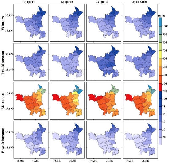
Figure 3.
The long-term distribution of mean rainfall (mm per season) presented in QDT1 in (a), QDT2 in (b), QDT3 in (c), and CLM120 in (d) and seasons, viz: winter season (JF; row 1st), pre-monsoon season (MAM; row 2nd), monsoon season (JJAS; row 3rd) and post-monsoon season (OND; row 4th) in the districts of Haryana state of India.
4.1.2. Rainfall Deviation
Figure 4 portrays the visuals of spatio-temporal variation of PDR during different seasons at the district level in different QDTs against CLM120. The positive PDR depicts above-normal rainfall, and the negative PDR depicts BNR. It can be observed that most of the districts received the above-normal rainfall during QDT1 in winter and post-monsoon seasons; however, BNR trend is apparent in most of the districts in pre-monsoon and monsoon seasons. The BNR trend was observed during QDT2 and QDT3 in winter season. Pre-monsoon season rainfall has shown an increasing trend during the last QDT; however, the most negative deviations were observed in QDT2. Negative PDR during the QDT3 depicts the decreasing trend of rainfall in most of the districts in the winter, summer monsoon, and post-monsoon seasons in recent times. Overall, no synchronized trend of deviation in any particular season was observed in all three QDTs. Rainfall during winter and pre-monsoon seasons have shown positive rainfall deviation in all districts during QDT1 and QDT3, respectively. However, both monsoon and post-monsoon seasons have shown a positive trend of rainfall deviation in all districts during QDT2. Overall, we can conclude that rainfall is decreasing during winter, monsoon, and post-monsoon seasons while it is increasing in pre-monsoon season in the last QDT, i.e., during recent climate. This change in rainfall pattern can be due to the high rate of climate change during recent years [39,76,77].
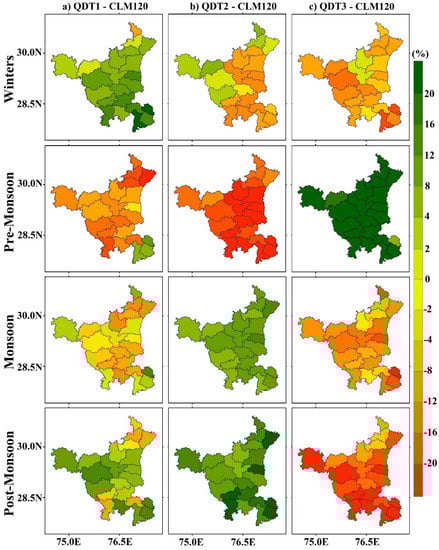
Figure 4.
The long term per-cent Rainfall Deviation (%) in QDT1 in (a), QDT2 in (b), and QDT3 in (c) from CLM120, and season, viz: winter season (JF; row 1st), pre-monsoon season (MAM; row 2nd), monsoon season (JJAS; row 3rd), and post-monsoon season (OND; row 4th) in the districts of Haryana state of India.
4.1.3. Rainfall Variability and Categorisation
The spatial variability in the seasonal rainfall of Haryana over the course of the study period is expressed by coefficient of variation (CV) in Figure 5. A large CV is indicative of large spatial variability and vice-versa. The value of CV was observed highest during post-monsoon, while it was lowest for monsoon season. Among districts, the variability of rainfall was higher in the districts lying in western Haryana.
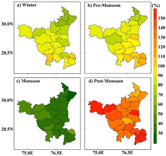
Figure 5.
The long-term distribution of coefficient of variation of seasonal rainfall during winter season (JF; in (a)), pre-monsoon season (MAM; in (b)), monsoon season (JJAS; in (c)), and post-monsoon season (OND; in (d)) in the districts of Haryana state of India.
Inter-annual variability in the seasonal rainfall of whole state and the categorization (large excess, excess, normal, deficient, and large deficient) in the seasonal rainfall of different districts of Haryana over the course of the study period from 1901 to 2020 is shown in Figure 6. The blue area shows the positive anomaly, and the red area shows the negative anomaly of seasonal rainfall from long term mean while the light purple shaded area shows the 11 years moving average of the annual rainfall of the whole state respectively in inter-annual variability plots. During winter season, a negative anomaly was witnessed in Haryana during the years 1902, 1903, 1904, 1925, 1932, 1946, 1958, 1960, 1963, 1964, 1967, 1969, 1974, 1980, 1988, 1997, 2006, 2008, 2012, 2016, and 2018 while different districts received deficient to large deficient rainfall in these corresponding years. Overall, the normal rainfall was found in 20% of the cases while deficient and large deficient categories were observed in 45.8% cases during the winter season. During the pre-monsoon season, a diminution in seasonal rainfall was observed from 1918 till 1975 and from 1988 to 1998, while an increase from 1977 to 1987 and from post-1999 to till now was observed. Deficient to large deficient rainfall was received in about 51.7% of the events during the years 1903, 1910, 1921, 1922, 1924, 1925, 1928, 1929, 1930, 1949, 1953, 1954, 1958, 1961, 1974, 1975, 1984, 1985, 1992, 1996, 2003, and 2010 in all of the districts of Haryana. Rainfall during the summer monsoon season increased from 1950 to 1975, then declined in the last decade of the study period. Normal monsoon rainfall was observed in 43.3% of the events, whereas deficient to large deficient rainfall in all the districts was observed in 30% of rainfall events of monsoon season during the year 1905, 1907, 1915, 1918, 1928, 1929, 1938, 1939, 1940, 1941, 1951, 1979, 1982, 1987, 1999, 2002, 2004, 2006, 2014, 2015 and 2019. Post-monsoon rainfall rose from 1950 to 1964 and dropped from 1933 to 1949, and from 2003 to the end of the study period. Deficient to large deficient rainfall was witnessed in 58.3% of rainfall occasions in all of the districts during the year 1901, 1905, 1907, 1908, 1918, 1920, 1926, 1930, 1939, 1940, 1941, 1943, 1945, 1949, 1950, 1952, 1969, 1976, 1978, 1984, 1993, 1994, 1995, 2000, 2005, 2007, 2011, 2012, 2015, and 2017, specifically in the large deficient category whereas normal rainfall was observed only in 12.5% during the post-monsoon rainfall season. However, rainfall during each season in the entire state showed epochal variations during the entire investigation span, but the magnitude and range of fluctuation was widest during the monsoon and narrowest during the winter season. Overall, the most consistent rainfall events in the different districts of Haryana were noticed during the monsoon season, followed by winters, pre-monsoon, and post-monsoon season. Among different districts, the ones lying in the eastern Haryana showed less variability as compared to the ones lying in western Haryana. This can be attributed to the comparatively higher altitude because of the presence of the foothills of Himalayas in the north-eastern Haryana, which facilitates the higher and most normal rainfall.
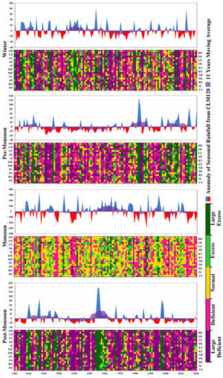
Figure 6.
The long term distribution of inter-annual variability of whole state (in 1st block) and the categorization in the different districts of Haryana state of India (in 2nd block) of seasonal rainfall during winter season (JF), pre-monsoon season (MAM), monsoon season (JJAS) and post-monsoon season (OND) as per IMD classification presented in blocks a–d, respectively, where large excess (≥60% from CLM120) is represented by dark green, excess (20% to 59% from CLM120) is represented by light green, normal (−19% to +19% from CLM120) is represented by yellow, deficient (−59% to −20%) is represented by magenta, and large-deficient (≤−60% from CLM120) is represented by purple.
4.2. Distribution Pattern of Rainfall
4.2.1. Rainfall Trend
The innovative trend analysis (ITA) was applied to detect the trends in time series of rainfall in different QDT’s as well as CLM120. Traditional studies, which usually consider a whole time period, give an outlook of overall changes acquainted at any region, but this type of trend analysis is helpful in detecting the significant changes encountered during specific time period, which can direct the researchers and policy makers in identifying the probable cause of these changes at that particular point of time, thus giving them a narrower study window than considering a broad temporal scale.
The rainfall trends in winter season detected by ITA are given in Table 2 and the ITA graphical results can be clearly seen in Figure 7. It is obvious that ITA slopes (ITAS) are dominated by negative values, and all of them (except CD) are significant (p < 0.01) whereas only PK showed significantly positive (p < 0.01) trend during CLM120. During QDT1 of winter season, the ITAS reveal that about 68.18% of districts are statistically significant at either 95% or 99% confidence level. Among them, the increasing trend was observed in 22.7% districts specifically located in north-eastern Haryana, whereas a decreasing trend was observed in 45.5% of the districts scattered over the study area. About 86.4% of the districts showed a statistically significant decreasing trend, whereas CD was the only district which encountered a statistically significant rising trend at 99% confidence level during QDT2. During QDT3, about 49.9% of districts showed statistically significant increasing trend at 99% confidence level. Among them, the increasing trend was observed in 22.7% districts specifically located in eastern Haryana whereas, decreasing trend was observed in 45.5% of the districts scattered over the study area. Overall, decreasing trend along with highest degree of change in magnitude in most of the district were observed during QDT2.
Table 2.
Results of innovative trend analysis during winter season at district level in Haryana during different time periods.
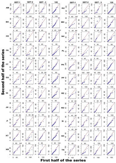
Figure 7.
Innovative trend analysis of winter season (JF) rainfall during QDT1, QDT2, QDT3, and CLM120 in the different districts of Haryana, India.
The rainfall trends in pre-monsoon season detected by ITA are given in Table 3, and its graphical illustrations can be evidently seen from Figure 8. It is obvious that ITAS is predominantly inclined towards the positive side for all the districts, and all of them are significant (p < 0.01) except FR only, which showed a significantly negative (p < 0.01) trend during CLM120. During QDT1 of pre-monsoon season, the ITAS disclose that all of the districts showed a statistically significant decreasing trend at 99% confidence level except FR only, which showed non-significantly increasing trend. Statistically significant escalating trend during QDT1 was observed in 72.7% of the districts, whereas a significantly decreasing trend was observed only in two of the districts, i.e., FR and PL, lying at the south-eastern border of Haryana at 99% confidence level. During QDT3 of pre-monsoon season, the ITAS tell that about 68.18% of districts are statistically significant at 99% confidence level. Among them, the increasing trend was observed in 54.5% districts whereas, decreasing trend was observed in 13.6% of the districts lying in north-eastern parts of the study area. Overall, an increasing trend in pre-monsoon rainfall was observed in almost all of the districts of Haryana during the last 2 QDTs.
Table 3.
Results of innovative trend analysis during pre-monsoon season at district level in Haryana during different time periods.
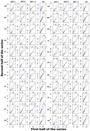
Figure 8.
Same as Figure 7 except for the pre-monsoon (MAM).
The rainfall trends in monsoon season detected by ITA are given in Table 4 and the ITA graphical results can be seen in Figure 9. The ITAS reveal that about 81.8% of districts showed a statistically significant trend at 99% confidence level. Among them, the increasing (36.4%) and the decreasing (45.4%) trends are almost equally dominating all over the study area during CLM120. During QDT1 of monsoon season, only 50.0% of the districts showed statistically significant trend at either 95% or 99% confidence level. Among them, the increasing trend was observed in 13.6%, whereas a decreasing trend was observed in 36.4% of the districts. About 77.3% of the districts showed a statistically significant trend at 99% confidence level, out of which 40.9% showed a rising trend whereas 36.4% showed a falling trend in monsoon rainfall during QDT3. During QDT3, about 72.7% of the districts showed statistically significant decreasing trend, whereas only two districts, i.e., CD and MH showed statistically significant rising trend in monsoon rainfall at 99% confidence level. Overall, a decreasing trend accompanied by highest degree of change in magnitude in most of the district were observed in the recent times (QDT3).
Table 4.
Results of innovative trend analysis during monsoon season at district level in Haryana during different time periods.
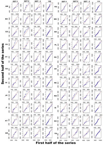
Figure 9.
Same as Figure 7 except for the monsoon season (JJAS).
The rainfall trends in post-monsoon season spotted by ITA are given in Table 5 with its plots can be seen from Figure 10. It is obvious that ITAS are predominantly inclined towards the negative side for all the districts, and all of them are significant (p < 0.01) except AM only, which showed a non-significantly negative trend during CLM120. During QDT1 of post-monsoon season, the ITAS disclose that only 40.9% of the districts showed a statistically significant trend at 99% confidence level out of which 22.7% districts noticed rising whereas 18.2% districts noticed falling trend in post-monsoon rainfall. A statistically significant decreasing trend was observed during both QDT2 and QDT3 in 95.5% and 90.9% of the districts, respectively. Overall, a decreasing trend in post-monsoon rainfall was observed in almost all of the districts lying in the study area during last two QDTs. The presence of these significant trends indicates towards the impact of climate change on the rainfall pattern of Haryana [76].
Table 5.
Results of innovative trend analysis during post-monsoon season at district level in Haryana during different time periods.
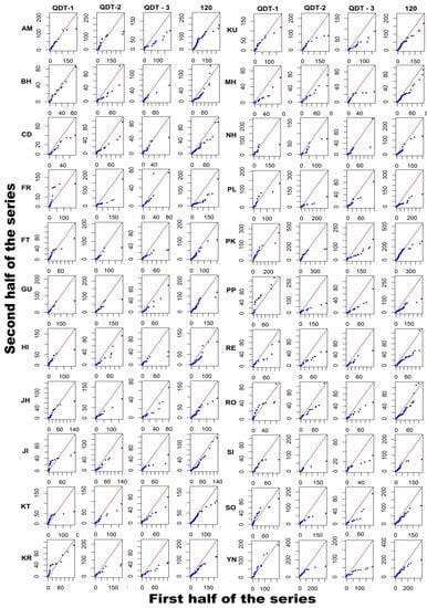
Figure 10.
Same as Figure 7 except for the post-monsoon season (OND).
From this study, it is apparent that significant changes were observed in each season for the whole study period, but we were able to identify the specific time period in which significant changes were detected with greater magnitude of slope in each season. We compared the results of our study with many similar analyses performed by different researchers. Guhathakurta et al. [78] examined the monthly, seasonal, and annual data series of 30 years (1989–2018) for all districts of Haryana and found a significantly decreasing trend in AM, BH, CD KT, PK, and PP. Nain et al. [79] performed trend analysis at monthly scale for 27 rain gauge stations scattered in all the districts of Haryana State using datasets of IMD Pune for a period of 42 years (1970–2011) and reported mixed trends for stations. Malik and Singh also [80] explored rainfall pattern characteristics in the Haryana region during 1997–2014 at daily and seasonal scale and found positive trend in monthly maximum and total rainfall. Anurag et al. [81] performed monthly analysis of rainfall and reported variable results with somewhat increasing trends at HI and decreasing trends at SI in Haryana state. There are many other studies conducted on small scales for the study area that have used different approaches to detect trends in rainfall, such as the studies by Sharma and Jain [82] for SI district, Anurag et al. [83] for HI district, and Bemal et al. [84] over eastern agroclimatic zone of Haryana. Kaur et al. [85] reported decreasing trends in in lower Shivaliks of Punjab, an adjoining state to Haryana, India. The advantage of using ITA method over the other non-parametric methods used by different researchers [78,79,80,81,82,83,84,85] discussed in this section is that they were not able to detect the trends significantly, but ITA was able to detect significant trends at regional scale during all the seasons. Additionally, we found no other study in the literature prior to this that had explored the spatiotemporal trends in seasonal rainfall for a century-long period.
4.2.2. Correlation Analysis
In order to determine the complexity and behaviour of rainfall across different areas, the cross-correlation analysis was carried out for the different seasonal rainfall, which is shown in Figure 11. The value of cross-correlation coefficients (CCCs) of all the districts showed statistically significant (critical value at α = 0.01 level and n = 120 is 0.24) and positive correlation with rainfall of Haryana for each season. From the legend, it can be seen that the yellow colour corresponds to weak interaction and blue colour corresponds to strong interaction. During the winter season, PK shows weaker CCCs, while AM, JH, RO, SO, and YN demonstrate strong CCCs with different districts of Haryana. During the pre-monsoon season, JH, JI, KR, RO, and SO depicts higher CCCs, however, lower CCCs at PL and FR were observed with various districts of the state. During the monsoon season, rainfall at AM, FR, SI, and YN showed weaker CCCs with different districts of Haryana. During the post-monsoon season, BH, CD, JH, KR, KU, SO, and RO have shown strong CCCs, however, FR, NH, and PL have weaker CCCs with various districts of Haryana. Overall, districts lying in eastern Haryana during the winter season have shown higher CCCs with different districts of Haryana, i.e., the rainfall occurring in the districts lying in eastern Haryana covers a larger area. The districts lying in central Haryana cover a broader area of the state during rainfall events in the pre-monsoon season. In spite of the higher MR at AM and YN, the CCC value of rainfall during the monsoon season at these districts suggests that the distribution of the rainfall is confined and does not cover a broader area of the rest of the state. This can be attributed to the higher elevation of these places, which triggers orographic precipitation leading to a localized phenomenon. During the post-monsoon season, the rainfall occurring in the south-eastern districts of Haryana has narrow distribution owing to the weaker CCCs values.
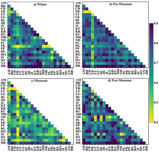
Figure 11.
The cross-correlation analysis of rainfall between different districts of Haryana during winter season (JF; in (a)), pre-monsoon season (MAM; in (b)), monsoon season (JJAS; in (c)), and post-monsoon season (OND; in (d)) at 1% level of significance, where correlation coefficient is increasing from yellow to blue.
4.2.3. Probability Distribution Function
Seasonal rainfall frequency was projected to generate a probability distribution function (PDF) across various deviation levels from normal rainfall (Figure 12). The PDF clearly shows more probability towards negative deviation categories, i.e., lower rainfall values in all the seasons. The winter rainfall frequency has two peaks near around 60% and −20% deviation from normal seasonal rainfall. The pre-monsoon frequency also peaks around the large deficient category of rainfall. The monsoon rainfall was observed highest near 20% rainfall departure from normal seasonal rainfall on the negative side. The frequency of post-monsoon rainfall decreased gradually towards positive from the negative deviation of the normal rainfall. Overall, the highest peak of rainfall frequency was below normal for all the seasons. This indicates an increase in the probability of having below normal rainfall in all the seasons which may enhance the risk of water security in the state.
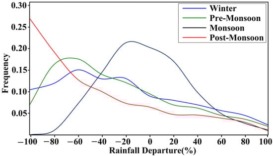
Figure 12.
The Probability Distribution Function of rainfall across various deviation levels from normal seasonal rainfall (%) during winter season (JF; blue line), pre-monsoon season (MAM; green line), monsoon season (JJAS; black line) and post-monsoon season (OND; red line).
4.2.4. Atmospheric Dynamics during Heavy Rainfall Events (HREs)
The precipitation features are estimated using surface and atmospheric meteorological variables to study heavy rainfall events [86] on a regional scale, which here covers the area between 73–80° E and 27–32° E. Based on the availability of the data, the HREs with a minimum of four days spell received in the state of Haryana during each season were detected for 1981–2020. The atmospheric meteorological variables like lower wind circulation at 850 hPa (m/s), VIMT (kg/m/s), and PWC (mm) are good indicators of the heavy rainfall event. HREs basically depend on low-level moisture convergence [87], as evaporation alone is not enough to increase a considerable amount of moisture to cause moderate or heavy rainfall. The increasing amount of water vapor content in the atmosphere increases the convergence of moisture thus leading to higher chances of HREs, and the rainfall intensity further increases because of additional moisture supplied due to the release of latent heat [15,88,89]. The orographic features also trigger the HREs at synoptic-scale in the mountainous regions [90,91,92,93]. We have identified 10–13 February 2007, 15–18 April 1983, 3–6 September 1995, and 16–19 October 1998 as the HREs in Haryana during the winter, pre-monsoon, summer monsoon, and post-monsoon seasons, respectively. The daily distribution of rainfall and atmospheric variables over the region for the winter season during 10–13 February 2007 is illustrated in Figure 13. Figure 13a shows that Haryana encountered HREs with a distribution of above 70 mm rainfall during the second and third days mostly confined to north-eastern districts. In the sectors of heavy rainfall, the lower atmosphere had south-westerly cyclonic flow with south-easterly winds blowing at a speed of 15 m/s and 9 m/s on the second and third day, respectively (Figure 13b). The maximum amount of atmospheric moisture depicted here as PWC, accumulated over south-western Haryana on the second and third days was in the range of 70–80 mm and 60–70 mm. The highest vertical transport of atmospheric moisture was observed on the second and third days in the range of 1800 kg/m/s and 1000 kg/m/s in the state of Haryana and adjoining regions respectively. On 11 February 2007, the state of Haryana and adjoining regions received the highest amount of rainfall along with strong north-easterly low-level jet and maximum moisture transport. The HREs observed in the pre-monsoon season during 15–18 April 1983 show the spatial distribution of rainfall ranging up to 70 mm from 1st to 3rd days, covering most of the districts of Haryana and adjoining regions. The low-level wind had south-westerly cyclonic flow with stronger south-easterly winds blowing at 15 m/s on the second day (Figure 14b). The highest PWC was seen in the southern region of Haryana for the 1st day, whereas it covered districts lying in north-eastern Haryana on the 2nd and 3rd days ranging 70–90 mm (Figure 14c). The highest VIMT ranging around 1400 kg/m/s and 1000 kg/m/s was observed on 2nd and 3rd days with flow directed towards the southeast direction in the state of Haryana and adjoining regions (Figure 14d). Overall, heavy rainfall was reported on 16–17 April in the year 1983 during pre-monsoon season over the state of Haryana and neighbouring areas, where strong north-easterly low-level jets aided in moisture transport. The heaviest rainfall event in the southwest monsoon season throughout the course of study period was witnessed during 3–6 September 1995 (Figure 15). The heavy rainfall of about 200 mm was observed during 4–5 September 1995 in various scattered pockets covering most of districts of Haryana and the adjoining regions (Figure 15a). The low-level atmospheric flow had shown the same behaviour on 1st and 4th days with westerly winds blowing at a speed of 6–9 m/s, whereas south-easterly wind flow at a speed of 9–15 m/s was observed on the 2nd day, however during the 3rd day, north-westerly winds blowing at 6–9 m/s were prevalent in western Haryana and south-easterly winds blowing at 12–21 m/s were prevalent in eastern Haryana (Figure 15b). The summer monsoon season PWC had values above 160 mm over the south-eastern and central regions on the 2nd and 3rd days (Figure 15c). The atmospheric moisture transport was having value in the range of 1800–2100 kg/m/s with south-easterly flow over the region during 3–5 September 1995. The heaviest rainfall event in the post-monsoon during the study period was observed on 16–19 October 1998 with a rainfall distribution of nearly 70 mm during the second and third days over the state Haryana (Figure 16). The lower atmospheric winds had south-easterly cyclonic flow with strength of 15 m/s and 9 m/s on the 2nd and 3rd days, respectively (Figure 16b). Total PWC had a southern domain with maximum value of 120–130 mm, covering almost the whole state on the 2nd and 3rd day (Figure 16c). The VIMT had southwest domain with a value of 1200 kg/m/s on the 1st day, south-westerly to central domain with a value of 2100 kg/m/s on the 2nd day, and north-easterly domain with a value of 1500 kg/m/s on the 3rd day with respect to Haryana state.
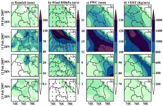
Figure 13.
The daily spatial distribution of heavy rainfall event for the winter season during 10–13 February 2007 of rainfall (IMD gridded datasets) is presented in (a) rainfall (mm), and analysis atmospheric variables (ECMWF reanalysis products) are presented in (b) wind at 850 hPa pressure level (magnitude in m/s and direction in arrow), (c) PWC between the surface to 300 hPa pressure level (mm) and (d) VIMT between the surface to 300 hPa pressure level (kg/m/s), respectively.
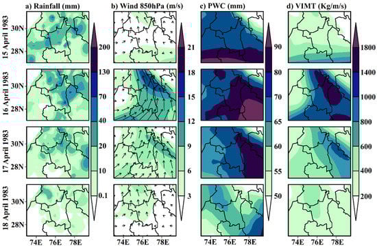
Figure 14.
The daily spatial distribution of heavy rainfall event for the pre-monsoon season during 15–18 April 1983 of rainfall (IMD gridded datasets) is presented in (a) rainfall (mm), and analysis atmospheric variables (ECMWF reanalysis products) are presented in (b) wind at 850 hPa pressure level (magnitude in m/s and direction in arrow), (c) PWC between the surface to 300 hPa pressure level (mm) and (d) VIMT between the surface to 300 hPa pressure level (kg/m/s), respectively.
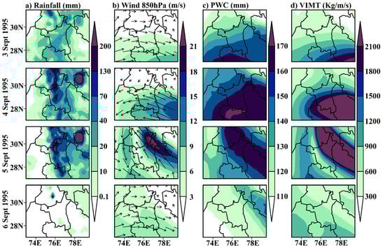
Figure 15.
The daily spatial distribution of heavy rainfall event for the monsoon season during 3–6 September 1995 of rainfall (IMD gridded datasets) is presented in (a) rainfall (mm), and analysis atmospheric variables (ECMWF reanalysis products) are presented in (b) wind at 850 hPa pressure level (magnitude in m/s and direction in arrow), (c) PWC between the surface to 300 hPa pressure level (mm) and (d) VIMT between the surface to 300 hPa pressure level (kg/m/s), respectively.
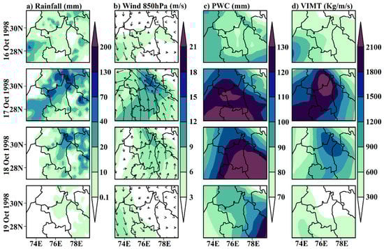
Figure 16.
The daily spatial distribution of heavy rainfall event for the post-monsoon season during 16–19 October 1998 of rainfall (IMD gridded datasets) is presented in (a) rainfall (mm), and analysis atmospheric variables (ECMWF reanalysis products) are presented in (b) wind at 850 hPa pressure level (magnitude in m/s and direction in arrow), (c) PWC between the surface to 300 hPa pressure level (mm) and (d) VIMT between the surface to 300 hPa pressure level (kg/m/s), respectively.
5. Conclusions
In the present study, the dynamics of seasonal rainfall time series data of 120 years (1901–2020) for 22 districts of Haryana, India, were analysed using spatio-temporal patterns of mean rainfall, rainfall deviation, moving-average, rainfall categorization, rainfall trend, correlation analysis, probability distribution function and heavy rainfall events. The districts lying in the eastern Haryana had received higher rainfall in each season than the ones lying in its western counterpart. Rainfall during pre-monsoon season has shown positive rainfall deviation, while it was negative for all the other seasons during the QDT3, which is indicative of decreasing rainfall at most of the districts of Haryana during winter, monsoon, and post-monsoon seasons in recent times. Among different seasons, the magnitude of variation in rainfall was broadest for summer monsoon season rainfall. Among different rainfall categories, normal rainfall events were observed relatively higher during summer monsoon, whereas it was lowest during post-monsoon season. Innovative Trend Analysis (ITA) depicts that most of the districts during winters and post-monsoon season, while most of the districts during summer monsoon season have shown a decrease in rainfall, however, all the districts have shown escalation in rainfall during pre-monsoon season over the study period. The presence of these trends depicts the impact of climate change on rainfall. All the districts had statistically significant and positive correlation with rainfall of Haryana during each season. The frequency of rainfall has departed towards the negative side, suggesting decreasing rainfall patterns in Haryana.
The heavy rainfall events were identified, and the analysis of the surface and atmospheric rainfall parameters was performed at the regional scale. During the pre-monsoon and post-monsoon seasons, these heavy rainfall events were accompanied by higher low-level tropospheric wind of 15 m/s, and wind reached a speed of about 21 m/s during the winter and summer monsoon seasons. All four seasons had strong south-easterly flow over the north Haryana and adjoining regions. During these heavy rainfall events, an enhancement in the total atmospheric moisture was observed in the range of 80 mm/day during winter and pre-monsoon seasons, while it increased to 150 mm/day and 120 mm/day during monsoon and post-monsoon seasons, respectively. The highest PWC and VIMT values during the heavier rainfall events were observed in summer monsoon season followed by post-monsoon, pre-monsoon, and winter seasons. Overall, heavy rainfall events over Haryana state were associated with strong south-easterly low-tropospheric wind, enhanced total atmospheric moisture, and rise in the transport of vertically integrated moisture. Our results have quantified the qualitative and quantitative aspects of rainfall dynamics for seasonal rainfall in the districts of Haryana. Given the impact of climate change on Haryana’s changing rainfall pattern, such analysis, together with spatio-temporal maps, could be critical for planning well-organized water resource usage and also for district-level water management in a sustainable manner. The scope of such study can be extended to adjacent states like Punjab, Himachal Pradesh, Rajasthan, Uttarakhand, etc., lying in north-west India. The agricultural or other socio-economic activities can also be managed by taking into account the rainfall dynamics discussed in this paper.
Author Contributions
A.S.C. was involved in methodology, investigation, data analysis, preparation of figures, and writing original draft. R.K.S.M. performed climatological data analysis for Heavy Rainfall events. O.K., A.R., A.D. and S.S. were involved in conceptualization, methodology, visualization, writing review & editing. All authors have read and agreed to the published version of the manuscript.
Funding
This research received no external funding.
Institutional Review Board Statement
Not applicable.
Informed Consent Statement
Not applicable.
Data Availability Statement
The daily gridded rainfall data for conducting this study is openly available at https://www.imdpune.gov.in/Clim_Pred_LRF_New/Grided_Data_Download.html. (accessed on 20 September 2021).
Acknowledgments
The authors would like to thank the India Meteorological Department (IMD), Pune, and the European Centre for Medium-Range Weather Forecasts (ECMWF) for providing the daily rainfall time series data and atmospheric datasets used in this study, respectively. The authors would also like to thank the Department of Agricultural Meteorology, Chaudhary Charan Singh Haryana Agricultural University for providing necessary facilities during the course of research period.
Conflicts of Interest
The authors declare no conflict of interest.
References
- Gergis, J.; Henley, B.J. Southern Hemisphere rainfall variability over the past 200 years. Clim. Dyn. 2017, 48, 2087–2105. [Google Scholar] [CrossRef]
- Deng, S.; Yang, N.; Li, M.; Cheng, L.; Chen, Z.; Chen, Y.; Chen, T.; Liu, X. Rainfall seasonality changes and its possible teleconnections with global climate events in China. Clim. Dyn. 2019, 53, 3529–3546. [Google Scholar] [CrossRef]
- Singh, C.; Ganguly, D.; Sharma, P. Impact of West Asia, Tibetan Plateau and local dust emissions on intra-seasonal oscillations of the South Asian monsoon rainfall. Clim. Dyn. 2019, 53, 6569–6593. [Google Scholar] [CrossRef]
- Bisht, D.S.; Chatterjee, C.; Raghuwanshi, N.S.; Sridhar, V. Spatio-temporal trends of rainfall across Indian river basins. Theor. Appl. Climatol. 2018, 132, 419–436. [Google Scholar] [CrossRef]
- Talchabhadel, R.; Karki, R. Correction to: Assessing climate boundary shifting under climate change scenarios across Nepal. Environ. Monit. Assess. 2019, 191, 707. [Google Scholar] [CrossRef]
- Tito, T.M.; Delgado, R.C.; de Carvalho, D.C.; Teodoro, P.E.; de Almeida, C.T.; Junior, C.A.d.; Santos, E.B.d.; Júnior, L.A.S.d. Assessment of evapotranspiration estimates based on surface and satellite data and its relationship with El Niño–Southern Oscillation in the Rio de Janeiro State. Environ. Monit. Assess. 2020, 192, 449. [Google Scholar] [CrossRef]
- Ferreira, F.L.V.; Rodrigues, L.N.; da Silva, D.D. Influence of changes in land use and land cover and rainfall on the streamflow regime of a watershed located in the transitioning region of the Brazilian Biomes Atlantic Forest and Cerrado. Environ. Monit. Assess. 2021, 193, 16. [Google Scholar] [CrossRef]
- Teixeira, D.B.d.; Veloso, M.F.; Ferreira, F.L.V.; Gleriani, J.M.; do Amaral, C.H. Spectro-temporal analysis of the Paraopeba River water after the tailings dam burst of the Córrego do Feijão mine, in Brumadinho, Brazil. Environ. Monit. Assess. 2021, 193, 435. [Google Scholar] [CrossRef]
- Cook, B.I.; Smerdon, J.E.; Seager, R.; Coats, S. Global warming and 21st century drying. Clim. Dyn. 2014, 43, 2607–2627. [Google Scholar] [CrossRef]
- Gizaw, M.S.; Gan, T.Y. Impact of climate change and El Niño episodes on droughts in sub-Saharan Africa. Clim. Dyn. 2017, 49, 665–682. [Google Scholar] [CrossRef]
- Carrão, H.; Naumann, G.; Barbosa, P. Global projections of drought hazard in a warming climate: A prime for disaster risk management. Clim. Dyn. 2018, 50, 2137–2155. [Google Scholar] [CrossRef]
- Handmer, J.; Honda, Y.; Kundzewicz, Z.W.; Arnell, N.; Benito, G.; Hatfield, J.; Mohamed, I.F.; Peduzzi, P.; Wu, S.; Sherstyukov, B.; et al. Changes in impacts of climate extremes: Human systems and ecosystems. In Managing the Risks of Extreme Events and Disasters to Advance Climate Change Adaptation: Special Report of the Intergovernmental Panel on Climate Change; Cambridge University Press: Cambridge, UK, 2012; pp. 231–290. [Google Scholar] [CrossRef]
- Dore, M.H. Climate change and changes in global precipitation patterns: What do we know? Environ. Int. 2005, 31, 1167–1181. [Google Scholar] [CrossRef] [PubMed]
- Van Wageningen, A.; Du Plessis, J.A. Are rainfall intensities changing, could climate change be blamed and what could be the impact for hydrologists? Water SA 2007, 33, 571–574. [Google Scholar]
- Trenberth, K.E. Changes in precipitation with climate change. Clim. Res. 2011, 47, 123–138. [Google Scholar] [CrossRef]
- Kumar, V.; Jat, H.S.; Sharma, P.C.; Gathala, M.K.; Malik, R.K.; Kamboj, B.R.; Yadav, A.K.; Ladha, J.K.; Raman, A.; Sharma, D.K.; et al. Can productivity and profitability be enhanced in intensively managed cereal systems while reducing the environmental footprint of production? Assessing sustainable intensification options in the breadbasket of India. Agric. Ecosyst Environ. 2018, 252, 132–147. [Google Scholar] [CrossRef] [PubMed]
- Shirsath, P.B.; Jat, M.L.; McDonald, A.J.; Srivastava, A.K.; Craufurd, P.; Rana, D.S.; Singh, A.K.; Chaudhari, S.K.; Sharma, P.C.; Singh, R.; et al. Agricultural labor, COVID-19, and potential implications for food security and air quality in the breadbasket of India. Agric. Syst. 2020, 185, 102954. [Google Scholar] [CrossRef]
- Sihmar, R. Growth and instability in agricultural production in Haryana: A District level analysis. Int. J. Sci. Res. Pub. 2014, 4, 1–12. [Google Scholar]
- Nirmala, B.; Muthuraman, P. Economic and constraint analysis of rice cultivation in Kaithal district of Haryana. Indian Res. J. Ext. Edu. 2016, 9, 47–49. [Google Scholar]
- Singh, J. Paddy and wheat stubble blazing in Haryana and Punjab states of India: A menace for environmental health. Manag. Environ. Qual. 2018, 28, 47–53. [Google Scholar] [CrossRef]
- Kumar, V.; Kumar, D.; Kumar, P. Declining water table scenario in Haryana-A review. Water Energy Int. 2007, 64, 32–34. [Google Scholar]
- Chaudhuri, S.; Roy, M. Reflections on groundwater quality and urban-rural disparity in drinking water sources in the state of Haryana, India. Int. J. Sci. Res. Dev. 2016, 4, 837–843. [Google Scholar]
- Cengiz, T.M.; Tabari, H.; Onyutha, C.; Kisi, O. Combined use of graphical and statistical approaches for analyzing historical precipitation changes in the Black Sea region of Turkey. Water 2020, 12, 705. [Google Scholar] [CrossRef]
- Ay, M.; Kisi, O. Investigation of trend analysis of monthly total precipitation by an innovative method. Theor. Appl. Climatol. 2015, 120, 617–629. [Google Scholar] [CrossRef]
- Ahmad, I.; Zhang, F.; Tayyab, M.; Anjum, M.N.; Zaman, M.; Liu, J.; Farid, H.U.; Saddique, Q. Spatiotemporal analysis of precipitation variability in annual, seasonal and extreme values over upper Indus River basin. Atmos. Res. 2018, 213, 346–360. [Google Scholar] [CrossRef]
- Serencam, U. Innovative trend analysis of total annual rainfall and temperature variability case study: Yesilirmak region, Turkey. Arab. J. Geosci. 2019, 12, 704. [Google Scholar] [CrossRef]
- Tosunoglu, F.; Kisi, O. Trend analysis of maximum hydrologic drought variables using Mann–Kendall and Şen’s innovative trend method. River Res. Appl. 2017, 33, 597–610. [Google Scholar] [CrossRef]
- Kisi, O. An innovative method for trend analysis of monthly pan evaporations. J. Hydrol. 2015, 527, 1123–1129. [Google Scholar] [CrossRef]
- Kisi, O.; Ay, M. Comparison of Mann–Kendall and innovative trend method for water quality parameters of the Kizilirmak River, Turkey. J Hydrol. 2014, 513, 362–375. [Google Scholar] [CrossRef]
- Markus, M.; Demissie, M.; Short, M.B.; Verma, S.; Cooke, R.A. Sensitivity analysis of annual nitrate loads and the corresponding trends in the lower Illinois River. J. Hydrol. Eng. 2013, 19, 533–543. [Google Scholar] [CrossRef]
- Sa’adi, Z.; Shahid, S.; Ismail, T.; Chung, E.S.; Wang, X.J. Trends analysis of rainfall and rainfall extremes in Sarawak, Malaysia using modified Mann–Kendall test. Meteorol. Atmos. Phys. 2019, 131, 263–277. [Google Scholar] [CrossRef]
- Marumbwa, F.M.; Cho, M.A.; Chirwa, P.W. Analysis of spatio-temporal rainfall trends across southern African biomes between 1981 and 2016. Phys. Chem. Earth. 2019, 114, 102808. [Google Scholar] [CrossRef]
- Wang, Y.; Xu, Y.; Tabari, H.; Wang, J.; Wang, Q.; Song, S.; Hu, Z. Innovative trend analysis of annual and seasonal rainfall in the Yangtze River Delta, eastern China. Atmos Res. 2020, 231, 104673. [Google Scholar] [CrossRef]
- Jonah, K.; Wen, W.; Shahid, S.; Ali, M.A.; Bilal, M.; Habtemicheal, B.A.; Iyakaremye, V.; Qiu, Z.; Almazroui, M.; Wang, Y.; et al. Spatiotemporal variability of rainfall trends and influencing factors in Rwanda. J. Atmos. Sol.-Terr. Phys. 2021, 219, 105631. [Google Scholar] [CrossRef]
- Kumar, V.; Jain, S.K.; Singh, Y. Analysis of long-term rainfall trends in India. Hydrol. Sci. J. 2010, 55, 484–496. [Google Scholar] [CrossRef]
- Joshi, S.; Gouda, K.C.; Goswami, P. Seasonal rainfall forecast skill over Central Himalaya with an atmospheric general circulation model. Theor. Appl. Climatol. 2020, 139, 237–250. [Google Scholar] [CrossRef]
- Sahoo, S.K.; Ajilesh, P.P.; Gouda, K.C.; Himesh, S. Impact of land-use changes on the genesis and evolution of extreme rainfall event: A case study over Uttarakhand, India. Theor. Appl. Climatol. 2020, 140, 915–926. [Google Scholar] [CrossRef]
- Malik, A.; Kumar, A. Spatio-temporal trend analysis of rainfall using parametric and non-parametric tests: Case study in Uttarakhand, India. Theor. Appl. Climatol. 2020, 140, 183–207. [Google Scholar] [CrossRef]
- Patra, J.P.; Mishra, A.; Singh, R.; Raghuwanshi, N.S. Detecting rainfall trends in twentieth century (1871–2006) over Orissa State, India. Clim. Chang. 2012, 111, 801–817. [Google Scholar] [CrossRef]
- Krishnakumar, K.N.; Prasada Rao, G.S.L.H.V.; Gopakumar, C.S. Rainfall trends in twentieth century over Kerala, India. Atmos. Environ. 2009, 43, 1940–1944. [Google Scholar] [CrossRef]
- Prasad, A.K.; Singh, R.P. Extreme rainfall event of July 25–27, 2005 over Mumbai, west coast, India. J. Indian Soc. Remote Sens. 2005, 33, 365–370. [Google Scholar] [CrossRef]
- Ranger, N.; Hallegatte, S.; Bhattacharya, S.; Bachu, M.; Priya, S.; Dhore, K.; Rafique, F.; Mathur, P.; Naville, N.; Henriet, F.; et al. An assessment of the potential impact of climate change on flood risk in Mumbai. Clim. Chang. 2011, 104, 139–167. [Google Scholar] [CrossRef]
- Uniyal, A. Lessons from Kedarnath tragedy of Uttarakhand Himalaya, India. Curr. Sci. 2013, 105, 1472–1474. [Google Scholar]
- Kotal, S.D.; Roy, S.S.; Bhowmik, S.R. Catastrophic heavy rainfall episode over Uttarakhand during 16–18 June 2013–observational aspects. Curr. Sci. 2014, 25, 234–245. [Google Scholar]
- Chevuturi, A.; Dimri, A.P. Investigation of Uttarakhand (India) disaster-2013 using weather research and forecasting model. Nat. Hazards 2016, 82, 1703–1726. [Google Scholar] [CrossRef]
- Mishra, V.; Shah, H.L. Hydroclimatological perspective of the Kerala flood of 2018. J. Geological. Soc. Ind. 2018, 92, 645–650. [Google Scholar] [CrossRef]
- Hunt, K.M.; Menon, A. The 2018 Kerala floods: A climate change perspective. Clim. Dyn. 2020, 54, 2433–2446. [Google Scholar] [CrossRef]
- Mishra, A.K. Monitoring Tamil Nadu flood of 2015 using satellite remote sensing. Nat. Hazards 2016, 82, 1431–1434. [Google Scholar] [CrossRef]
- Seenirajan, M.; Natarajan, M.; Thangaraj, R.; Bagyaraj, M. Study and analysis of Chennai flood 2015 using GIS and multicriteria technique. J. Geogr. Inf. Syst. 2017, 9, 126. [Google Scholar] [CrossRef][Green Version]
- Krishnamurthy, L.; Vecchi, G.A.; Yang, X.; van der Wiel, K.; Balaji, V.; Kapnick, S.B.; Jia, L.; Zeng, F.; Paffendorf, K.; Underwood, S. Causes and probability of occurrence of extreme precipitation events like Chennai 2015. J. Clim. 2018, 31, 3831–3848. [Google Scholar] [CrossRef]
- Devi, N.N.; Sridharan, B.; Kuiry, S.N. Impact of urban sprawl on future flooding in Chennai city, India. J. Hydrol. 2019, 574, 486–496. [Google Scholar] [CrossRef]
- Sen, R.S.; Balling, R.C. Trends in extreme daily precipitation indices in India. Int. J. Climatol. 2004, 24, 457–466. [Google Scholar] [CrossRef]
- Goswami, B.N.; Venugopal, V.; Sengupta, D.; Madhusoodanan, M.S.; Xavier, P.K. Increasing trend of extreme rain events over India in a warming environment. Science 2006, 314, 1442–1445. [Google Scholar] [CrossRef] [PubMed]
- Rajeevan, M.; Bhate, J.; Jaswal, A.K. Analysis of variability and trends of extreme rainfall events over India using 104 years of gridded daily rainfall data. Geophys. Res. Lett. 2008, 35, 1–6. [Google Scholar] [CrossRef]
- Vittal, H.; Karmakar, S.; Ghosh, S. Diametric changes in trends and patterns of extreme rainfall over India from pre-1950 to post-1950. Geophys. Res. Lett. 2013, 40, 3253–3258. [Google Scholar] [CrossRef]
- Abhilash. Growth and Radiation Use Efficiency of Basmati Rice (Oryza sativa L.) Varieties under Different Transplanting Environments. Master’s Thesis, CCS Haryana Agricultural University, Hisar, India, 2016; p. 36. [Google Scholar]
- Pai, D.S.; Sridhar, L.; Rajeevan, M.; Sreejith, O.P.; Satbhai, N.S.; Mukhopadhyay, B. Development of a new high spatial resolution (0.25° × 0.25°) long period (1901–2010) daily gridded rainfall data set over India and its comparison with existing data sets over the region. Mausam 2014, 65, 1–18. [Google Scholar] [CrossRef]
- Berrisford, P.; Kållberg, P.; Kobayashi, S.; Dee, D.; Uppala, S.; Simmons, A.J.; Poli, P.; Sato, H. Atmospheric conservation properties in ERA-Interim. Q. J. R. Meteorol. Soc. 2011, 137, 1381–1399. [Google Scholar] [CrossRef]
- Dee, D.P.; Uppala, S.M.; Simmons, A.J.; Berrisford, P.; Poli, P.; Kobayashi, S.; Andrae, U.; Balmaseda, M.A.; Balsamo, G.; Bauer, D.P.; et al. The ERA-Interim reanalysis: Configuration and performance of the data assimilation system. Q. J. R. Meteorol. Soc. 2011, 137, 553–597. [Google Scholar] [CrossRef]
- Khan, U. Emerging Trends of Urbanization in India: An Evaluation From Environmental Perspectives. Ph.D. Thesis, Aligarh Muslim University, Aligarh, India, 2011. [Google Scholar]
- Nomura, C. Historical roots of industrialisation and the emerging state in Colonial India. In Paths to the Emerging State in Asia and Africa, Emerging-Economy State and International Policy Studies; Springer: Singapore, 2019; pp. 169–193. [Google Scholar] [CrossRef]
- Tilman, D. The greening of the green revolution. Nature 1998, 396, 211–212. [Google Scholar] [CrossRef]
- Davidson, E.A. The contribution of manure and fertilizer nitrogen to atmospheric nitrous oxide since 1860. Nat. Geosci. 2009, 2, 659–662. [Google Scholar] [CrossRef]
- Kasliwal, R. The New Green Revolution: A Just Transition to Climate-Smart Crops. In ORF Issue Brief No. 433, January 2021; Observer Research Foundation: New Delhi, India, 2021. [Google Scholar]
- Saha, S.; Loveridge, J. Lessons learned from India’s Green Revolution: Why the Green Revolution is highly relevant for today’s world of pandemics, food insecurity, and uncertainty. TATuP-Z. Für Tech. Theor. Und Prax. J. Technol. Assess. Theory Pract. 2020, 29, 58–61. [Google Scholar] [CrossRef]
- Şen, Z. Innovative trend analysis methodology. J. Hydrol. Eng. 2012, 17, 1042–1046. [Google Scholar] [CrossRef]
- Pour, S.H.; Wahab, A.K.A.; Shahid, S.; Ismail, Z.B. Changes in reference evapotranspiration and its driving factors in peninsular Malaysia. Atmos. Res. 2020, 246, 105096. [Google Scholar] [CrossRef]
- Şen, Z. Innovative trend significance test and applications. Theor. Appl. Climatol. 2017, 127, 939–947. [Google Scholar] [CrossRef]
- Godfred-Spenning, C.R.; Reason, C.J. Interannual variability of lower-tropospheric moisture transport during the Australian monsoon. Int. J. Climatol. 2002, 22, 509–532. [Google Scholar] [CrossRef]
- Fasullo, J.; Webster, P.J. A hydrological definition of Indian monsoon onset and withdrawal. J. Clim. 2003, 16, 3200–3211. [Google Scholar] [CrossRef]
- Durai, V.R.; Bhowmik, S.R. Prediction of Indian summer monsoon in short to medium range time scale with high resolution global forecast system (GFS) T574 and T382. Clim. Dyn. 2014, 42, 1527–1551. [Google Scholar] [CrossRef]
- Maurya, R.K.S.; Sinha, P.; Mohanty, M.R.; Mohanty, U.C. RegCM4 model sensitivity to horizontal resolution and domain size in simulating the Indian summer monsoon. Atmos. Res. 2018, 210, 15–33. [Google Scholar] [CrossRef]
- Singh, P.; Kumar, N. Effect of orography on precipitation in the western Himalayan region. J. Hydrol. 1997, 199, 183–206. [Google Scholar] [CrossRef]
- Kuraji, K.; Punyatrong, K.; Suzuki, M. Altitudinal increase in rainfall in the Mae Chaem watershed, Thailand. J. Meteorol. Soc. Japan 2001, 79, 353–363. [Google Scholar] [CrossRef][Green Version]
- Shrestha, D.; Singh, P.; Nakamura, K. Spatiotemporal variation of rainfall over the central Himalayan region revealed by TRMM Precipitation Radar. J. Geophys. Res. Atmos. 2012, 117. [Google Scholar] [CrossRef]
- Krishnan, R.; Sanjay, J.; Gnanaseelan, C.; Mujumdar, M.; Kulkarni, A.; Chakraborty, S. Assessment of Climate Change over the Indian Region: A Report of the Ministry of Earth Sciences (MOES), Government of India; Springer: Berlin/Heidelberg, Germany, 2020; pp. 23–28. [Google Scholar]
- Praveen, B.; Talukdar, S.; Mahato, S.; Mondal, J.; Sharma, P.; Islam, A.R.M.; Rahman, A. Analyzing trend and forecasting of rainfall changes in India using non-parametrical and machine learning approaches. Sci. Rep. 2020, 10, 10342. [Google Scholar] [CrossRef] [PubMed]
- Guhathakurta, P.; Narkhede, N.; Menon, P.; Prasad, A.K.; Sangwan, N. CRS-IMD, Observed Rainfall Variability and Changes over Haryana State (2020). In Met Monograph No.: ESSO/IMD/HS/Rainfall Variability/09(2020)/33; Ministry of Earth Sciences, Government of India: New Delhi, India, 2020; pp. 43–56. [Google Scholar]
- Nain, M.; Hooda, B.K. Probability and trend analysis of monthly rainfall in Haryana. Int. J. Agri. Stat. Sci. 2019, 15, 221–229. [Google Scholar] [CrossRef]
- Malik, D.; Singh, K.K. Rainfall Trend Analysis of Various Districts of Haryana, India. In Sustainable Engineering; Springer: Singapore, 2019; pp. 95–109. [Google Scholar]
- Anurag, A.K.; Singh, D.; Singh, R.; Kumar, M.; Singh, S.; Kumar, S. Changes in weather entities and extreme events in western Haryana, India. J. Agrometeorol. 2018, 20, 135–142. [Google Scholar]
- Sharma, A.; Jain, K. Long-Term Trend Analysis of Rainfall Data of Sirsa Districts of Haryana. J. Water Res. Pollut. Stud. 2017, 2, 1–9. Available online: http://matjournals.in/index.php/JoWRPS/article/view/1436 (accessed on 21 February 2022).
- Anurag, A.K.; Singh, R.; Singh, D.; Kumar, M. Long Term Trends In Weather Parameters At Hisar (Haryana): A Location In Semi Arid Region of North West India. Int. J. Recent Sci. Res. 2017, 8, 18087–18090. [Google Scholar]
- Bemal, S.; Singh, D.; Singh, S. Rainfall variability analysis over eastern agroclimatic zone of Haryana. J. Agrometeorol. 2012, 14, 88–90. [Google Scholar]
- Kaur, N.; Yousuf, A.; Singh, M.J. Long term rainfall variability and trend analysis. Mausam 2021, 72, 571–582. [Google Scholar] [CrossRef]
- Liu, C.; Zipser, E.J. The global distribution of largest, deepest, and most intense precipitation systems. Geophys. Res. Lett. 2015, 42, 3591–3595. [Google Scholar] [CrossRef]
- Trenberth, K.E.; Dai, A.; Rasmussen, R.M.; Parsons, D.B. The changing character of precipitation. Bull. Am. Meteorol. Soc. 2003, 84, 1205–1218. [Google Scholar] [CrossRef]
- Trenberth, K.E. Atmospheric moisture residence times and cycling: Implications for rainfall rates and climate change. Clim. Change 1998, 39, 667–694. [Google Scholar] [CrossRef]
- Trenberth, K.E. Conceptual framework for changes of extremes of the hydrological cycle with climate change. In Weather and Climate Extremes; Springer: Dordrecht, The Netherlands, 1999; pp. 327–339. [Google Scholar] [CrossRef]
- Rao, Y.P. Meteorological Monograph on Synoptic Meteorology, No. 111976; Southwest Monsoon, India Meteorological Department: New Delhi, India, 1976; p. 337. [Google Scholar]
- Gadgil, S. Monsoon–ocean coupling. Curr. Sci. 2000, 10, 309–322. [Google Scholar]
- Sikka, D.R. A study on the monsoon low pressure systems over the Indian region and their relationship with drought and excess monsoon seasonal rainfall. COLA Tech. Rep. 2006, 217, 61. [Google Scholar]
- Krishnan, R.; Sabin, T.P.; Ayantika, D.C.; Kitoh, A.; Sugi, M.; Murakami, H.; Turner, A.G.; Slingo, J.M.; Rajendran, K. Will the south Asian monsoon overturning circulation stabilize any further? Clim. Dyn. 2013, 40, 187–211. [Google Scholar] [CrossRef]
Publisher’s Note: MDPI stays neutral with regard to jurisdictional claims in published maps and institutional affiliations. |
© 2022 by the authors. Licensee MDPI, Basel, Switzerland. This article is an open access article distributed under the terms and conditions of the Creative Commons Attribution (CC BY) license (https://creativecommons.org/licenses/by/4.0/).