Abstract
Short-range predictions of crop yield provide valuable insights for agricultural resource management and likely economic impacts associated with low yield. Such predictions are difficult to achieve in regions that lack extensive observational records. Herein, we demonstrate how a number of basic or readily available input data can be used to train an Artificial Neural Network (ANN) model to provide months-ahead predictions of cotton yield for a case study in Menemen Plain, Turkey. We use limited reported yield (13 years) along cumulative precipitation, cumulative heat units, two meteorologically-based drought indices (Standardized Precipitation Index (SPI) and Standardized Precipitation Evapotranspiration Index (SPEI)), and three remotely-sensed vegetation indices (Normalized Difference Vegetation Index (NDVI), Enhanced Vegetation Index (EVI), and Land Surface Water Index (LSWI)) as ANN inputs. Results indicate that, when EVI is combined with the preceding 12-month SPEI, it has better sensitivity to cotton yield than other indicators. The ANN model predicted cotton yield four months before harvest with R2 > 0.80, showing potential as a yield prediction tool. We discuss the effects of different combinations of input data (explanatory variables), dataset size, and selection of training data to inform future applications of ANN for early prediction of cotton yield in data-scarce regions.
1. Introduction
Early-in-the-growing season (i.e., short-range) predictions of crop yield are important for increasing productivity, managing economic losses due to low yield, and conserving natural resources. Short-range predictions of crop yield is important for managing the economic activity of the farm enterprise and for improved management of farm inputs (e.g., fertilizer, herbicides, etc.). As Leo et al. [1] stated, such short-range predictions for cotton could also lead to estimating revenue, gin workload, and market value. Moreover, short-range prediction tools could be of value in some cotton producing countries, such as Turkey, where irrigation water availability and management is a concern [2]. The IPCC (Intergovernmental Panel on Climate Change) projects a reduction in global crop yield with changing climate conditions [3] due to higher frequency, intensity and duration of drought [4,5]. At large scales, there is a need to develop, prioritize and implement strategies and policies for sustainable agricultural production [6,7,8]. However, at the local scale, producers need reliable, short-range yield prediction tools to enhance agricultural management systems in the face of uncertainties. Accurate, timely predictions of crop yield based on early indicators of water stress or untimely precipitation and variations of temperature is key for management of crucial farm resources for producers and for development of agricultural outlooks for traders and governments [9,10,11].
Reliable crop yield prediction depends on the choice of model, inputs to the model [12,13], and objective evaluation of the performance of the model. Hara et al. [12] provided a detailed description of factors influencing crop yields, which they divide into two broad categories, namely primary and secondary factors. Included within the primary factors are environmental indicators for example temperature and precipitation; soil characteristics such as pH and moisture, and nutrients; and agronomic factors for example land preparation, and planting date. While secondary factors are those that need additional measurements that use specialized devices and sensors—for example, remotely sensed vegetation indices. Artificial Neural Networks (ANNs) lend themselves for development and fine-tuning of data-driven predictive models as they employ past data [14,15,16,17,18]. ANNs are nonlinear models developed from a set of predictor variables and known outputs for use in predicting outcomes based upon new values of the predictors [19,20]. ANN results indicate that the model’s complexity and the size of training dataset affect the accuracy of predictions [21]. Statistical measures such as coefficient of determination (R2), percent bias (PBIAS) [22], and mean absolute percentage error (MAPE) [12] can be used to evaluate model performance.
Cotton is one of the most important and widely produced agricultural and industrial crops in the world [23], where Turkey ranks 6th in world production [24]. Additionally, cotton production in Turkey is the main livelihood for many farmers. Turkey’s export income from cotton is estimated to be ~$178 M annually [24]. The Menemen plain of Turkey is well known for the cultivation of cotton. However, there is no tool to estimate cotton yield for short-range prediction in Menemen.
This paper applies an ANN model to provide months-ahead predictions of cotton yield in data poor regions using basic or readily available climate and remote sensing data for the Menemen region of Turkey. With respect to climate, cotton is a plant that needs a long frost-free period, a lot of heat and plenty of sunshine, and prefers a warm and humid climate. Precipitation and temperature influence other climatic conditions such as relative humidity and soil temperature that affect cotton growth and yield [25,26]. In addition, Mauget et al. [27] showed that cotton planting date, which is determined by both soil moisture and soil temperature, affect cotton yield and quality with late planting, leading to reduced yield and quality. ANNs require numerous specific input parameters to train models, which are generally only available at data point locations [9]. As such, short-range predictions of yield are difficult to achieve in regions that lack extensive observational records. Crop yield models illustrate a strong relationship between yield, heat units, precipitation, drought indices, and vegetation indices [28,29,30,31]. Ref. [32] documented major effects of air temperature on cotton growth and yield. Air temperature for crop growth is generally expressed in heat units, which is average seasonal cumulative temperature within daily lower and upper crop growth thresholds [33]. Heat units and soil moisture are needed for crop germination and growth, which affect cotton yield [34]. Likewise, pre-season (January through April) precipitation affects cotton yield variability [25]. We used limited reported yield data (13 years) along with cumulative precipitation and cumulative heat units as basic inputs for the ANN model.
Previous studies have shown that drought and vegetation indices (VI) are useful for short-range crop predictions [35,36,37]. Ref. [38] used rainfall to estimate corn and soybean yield using ANN in Maryland, USA. The results showed that ANN corn yield model resulted in R2 = 0.77 and the soybean yield model R2 = 0.81. Recently, SPEI, SPI, and satellite based VIs were used in artificial intelligence-based crop yield forecasting models. For example, Ref. [39] showed that a forecasting system based on multiple growth stage-specific indicators, simulated biomass, climate extremes (drought, heat, and frost), NDVI, and SPEI can estimate wheat yield one month (~35 days) prior to harvest in southeastern Australia.
We used two meteorologically-based drought indices (Standardized Precipitation Index (SPI) and Standardized Precipitation Evapotranspiration Index (SPEI)), and three remotely-sensed VIs (Normalized Difference Vegetation Index (NDVI), Enhanced Vegetation Index (EVI), Land Surface Water Index (LSWI)) as early indicators of agricultural water stress. SPI [40] and SPEI [41] were developed to monitor meteorological drought and associated agricultural productivity. NDVI is a popular vegetation index, but it has some limitations since the index becomes saturated (i.e., non-responsive) to leaf area indexes due to lack of sensitivity to atmospheric aerosols and the soil background [42,43,44]. EVI was developed to minimize oversaturation when viewing land surfaces with high values of chlorophyll [45,46,47,48], and to enhance vegetation signals with an improved sensitivity to soil brightness [49,50]. LSWI is a water stress indicator [51], which is effective in representing free water, soil moisture, and vegetation water content [52,53]. Although LSWI is more sensitive to liquid water in vegetation canopies as compared to NDVI and EVI [54,55,56], its application has been limited to a small number of crops and climate conditions.
The overall goal of this study was to utilize a number of basic and readily available climate and remote sensing input data as explanatory variables for use by an ANN model to provide months ahead predictions of cotton yield for a case study in Menemen Plain, Turkey as an example of a data-scarce region. Specific objectives include determining (1) the effects of using different combinations of explanatory variables, also known as input neurons, on prediction accuracy, (2) the effects of dataset size and climate scenarios on prediction accuracy, and (3) possible lead-time to provide reasonably accurate cotton yield predictions for management decision-making. The use of meteorological and vegetation indices over different climate scenarios are presented as a numerical experiment of the ANN model’s ability to predict cotton yield under a range of plausible conditions. We discuss the effects of using different combinations of explanatory variables, dataset sizes, and selection of training data to inform future applications of ANN for early prediction of cotton yield in data-scarce regions.
2. Materials and Methods
2.1. Study Site
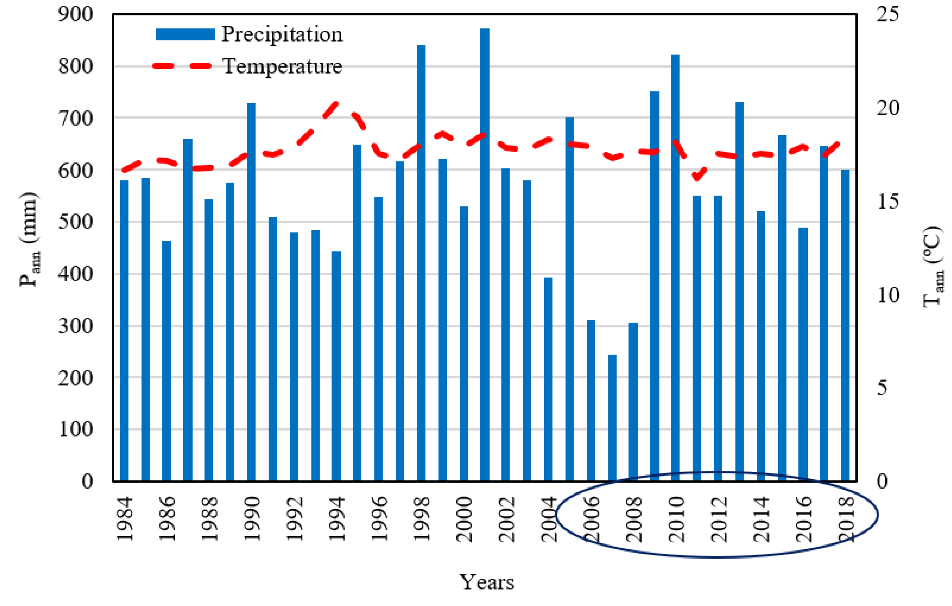
Turkey is located in the temperate zone of the Mediterranean basin and possesses many climate types [57]. However, ~42% of the country is largely characterized by the Koppen–Geiger Csa climate type, which includes western Turkey [57]. This study was carried out in the 69, 449 ha Menemen Plain of the lower Gediz River basin, which is located on the eastern edge of the Aegean Sea just north of Izmir, Turkey (26°40′–27°07′ E, 38°26′–38°40′ N). The Menemen Plain covers alluvial lands and colluvial foothills [58]. Gediz alluvial’s base is at an altitude of 0–6 m, and the side alluvials are at an altitude of 6–30 m. The nearby mountains’ altitude approaches 1100 m. The Menemen Plain, which is well known for the cultivation of cotton (8212 ha; 35% of total cultivated area), typifies a Mediterranean climate, with hot dry summers and cool wet winters. We acquired the long-term climate data for Menemen (1984 to 2018) from Turkish State Meteorological Service [59]. According to long-term climatic data (1984–2018), average total annual precipitation (Pann) is 577 mm, and average annual air temperature (Tann) is 18 °C (Figure 1). The hottest month is July and the coldest is January [59].
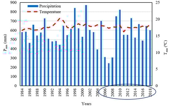
Figure 1.
Average annual temperature (Tann) and annual precipitation (Pann) for 1984–2018 (TSMS, 2020). The ellipse on the x-axis indicates the 13-year study period.
From 1984 through 2018, Pann varied from 245 mm (2007) to 822 mm (2001) and Tann ranged from 16.2 °C (2011) to 18.5 °C (1994). Moreover, the seasonal distribution of P (not shown) is also different between years. In this study, we used data for the period of 2006–2018, which is representative of the climatological conditions of the region. For this 13-year period, the total amount of precipitation was less than 8 mm in July–August and most precipitation occurred during September–March (data not shown), and generally irrigation starts in July for cotton growers in this region.
2.2. Measured Cotton Yield Data
The most common cotton variety grown in the Menemen Plain is upland cotton (Gossypium hirsutum) [60]. Cotton is usually planted between March–May and harvested between August and September. This study covers the growing period from April (planting) and September (harvesting) with flood irrigation generally starting in July [58]. Fertilizer application consists of mainly the standard nitrogen and phosphorus pentoxide (P2O5) applied at various rates though some research indicates benefits of potassium fertilizer [60]. Measured seed cotton yield data for the 2006 to 2018 period were obtained from the Turkish Statistical Institute [61]. The TSI collects data in various provinces/regions from the Ministry of Food, Agriculture, and Livestock and creates a summary of crop yields for each of the regions. The measured yields from 2006 to 2018 were 4810, 4790, 3850, 4990, 5350, 5470, 4680, 6000, 5950, 5430, 5410, 5190 and 5500 kg/ha, respectively [53].
2.3. Workflow, Explanatory ANN Variables, and Scenarios for Cotton Yield Prediction
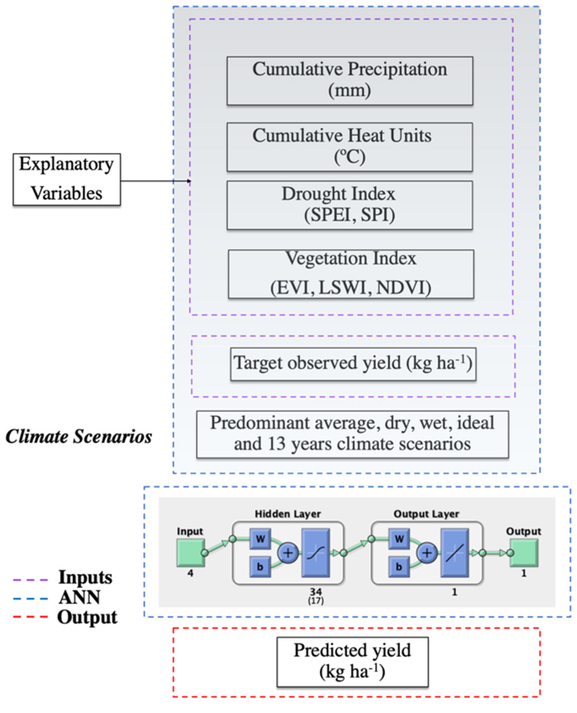
The general workflow for this study is depicted in Figure 2. Four categories of inputs were used in the development of the ANN models: meteorological data (P and heat units), drought indexes (SPEI, SPI; calculated from precipitation and air temperature data), vegetation indices (calculated from satellite data), and measured cotton yield. These inputs were used to train and evaluate the ANN for various climate scenarios representing predominantly average, dry, wet, and variable climate conditions using subsets of the 13-year record. From the climate dataset, four below average (blw; 2006, 2007, 2008 and 2016), four above average (abv; 2009, 2010, 2013 and 2015) and five average rainfall years (avg; 2011, 2012, 2014, 2017 and 2018) were selected to develop climate scenarios and train the ANN model. The variable climate scenarios were included in the analysis to subject the model to a variety of plausible conditions that capture year-to-year climate variability alongside the other more homogenous climate conditions for a comprehensive numerical experiment. In addition, the 13-year record was used as a baseline scenario.
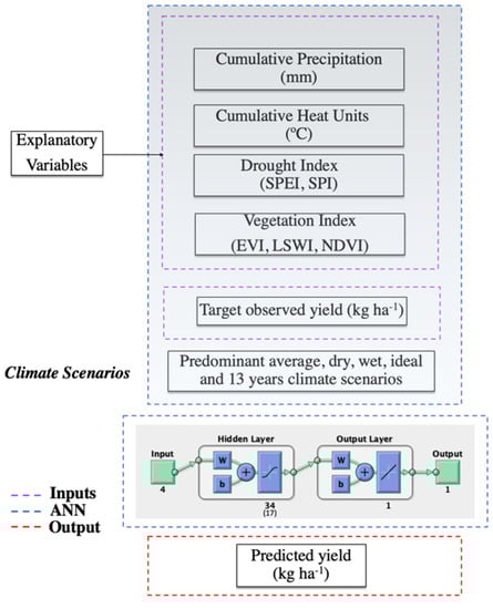
Figure 2.
General workflow for cotton yield prediction using ANN.
2.3.1. Explanatory Variables: Drought and Vegetation Indices, Heat Units, Precipitation
Two drought indices (DIs; i.e., SPI and SPEI) and three VIs (i.e., EVI, LSWI, and NDVI) were computed at different temporal scales, namely 3, 6, and 12 months, providing 18 combinations of indices (2 DIs × 3 VIs × 3 temporal scales). These indices were examined to determine the best combination of drought and vegetation indices to use together with cumulative precipitation (CP) and cumulative heat units (CHUs) in the ANN framework. The drought indices, vegetation indices, heat units, and precipitation are described below.
SPI: The SPI [32] is generally computed based on a 30-year long precipitation dataset with the accumulated precipitation values fit to a parametric statistical distribution from which non-exceedance probabilities are transformed to the standard normal distribution (µ = 0, σ = 1). A given SPI index value is computed by summing precipitation over n months, where n is typically 1, 3, 6, 9, 12, or 24 months [40,62,63] Equation (1). Table 1 gives a classification scheme for SPI index values:
where xi is the monthly precipitation amount (x1, x2, …, xn) and , s are the mean and standard deviation of the whole time series of monthly precipitation values [64].
SPEI: The SPEI [41] is similar to the SPI, but it takes into account potential evapotranspiration (ETp). For this study, SPEI was calculated based on monthly precipitation and ET using available data. In SPEI calculation, the difference (Di) between monthly or weekly precipitation (Pi) and potential evapotranspiration (ETpi) indicates water deficit or surplus, allowing to factor in the effects of temperature in drought characterization. Drought category classification based on SPEI value is summarized in Table 1:
Di = Pi-ETpi,
Details of the procedure to compute SPEI are given in Vicente Serrano et al. [41]. We used the Hargreaves [65] method to calculate ETp as modified by the FAO-56 reference crop definition [57]. The Hargreaves Equation (2) is based on the relationship between maximum and minimum air temperature as a proxy for net radiation [65]:
where Ra is the extraterrestrial radiation (MJ m−2 d−1), Tmax is maximum air temperature(°C), Tmin is the minimum air temperature (°C), Tavg is calculated as the average of Tmax and Tmin (°C), and the coefficient of 0.408 is used to convert from MJ m−2 d−1 to mm d−1. Ra is a function of latitude and day of year. Coefficients a (= 0.023), b (= 17.8), and c (= 0.5) are multiplier and offset parameters [65,66].

Table 1.
Drought category classification by SPI and SPEI values [40,67].
Table 1.
Drought category classification by SPI and SPEI values [40,67].
| SPI/SPEI Values | Drought Category |
|---|---|
| >2.00 | Extremely wet |
| 1.50 to 1.99 | Severely wet |
| 1.00 to 1.49 | Moderately wet |
| −0.99 to 0.99 | Near normal |
| −1.49 to −1.00 | Moderate drought |
| −1.99 to −1.50 | Severe drought |
| <−2.00 | Extreme drought |
Vegetation Indices (NDVI, EVI, LSWI): The Landsat 7 Enhanced Thematic Mapper Plus (ETM+) (30 m resolution) reflectance data in the blue (0.45–0.52 µm), green (0.52–0.60 µm), red (0.63–0.69 µm), near infrared (NIR: 0.77–0.90 µm), and two shortwave infrared (SWIR1: 1.55–1.75 µm, SWIR2: 2.09–2.35 µm) wavebands for the period 2006–2018 were obtained from the Google Earth Engine. Images having clouds and shadows were excluded from analysis. A total of 166 images were acquired with the number of images per year varying from 9 (2012) to 17 (2014, 2017, 2018) (Supplementary Table S1). Satellite images were acquired for path/row of 180/33 and 181/33 to provide a complete coverage of the study area. The images overlapped by ~20% because of the location of the study area in an overlap zone of the images. The overlap of the two images allowed observation of the study area on a less than 16-day basis.
The Landsat 7 ETM+ surface reflectance (ρ) from Landsat red, NIR, blue, and SWIR1 bands data were used to calculate NDVI [68], EVI [69] and LSWI [70] as shown in Equations (4)–(6):
The coefficient values used in the EVI equation are: G = 2.5, C1 = 6, C2 = 7.5, and L = 1 [50].
Heat Units: Heat units (HUs) were calculated using daily maximum (Tmax), minimum (Tmin) and base air temperature (Tb) expressed as:
In this study, Tb for cotton was assumed as 15.5 °C. Cumulative HUs (CHUs) were used. HUs computed for April when cotton was planted were used as CHUs. The value of CHUs for the months of May through August was calculated as the sum of heat units for all months from April through May, June, July, and August, respectively.
Cumulative Precipitation: Because antecedent soil moisture affects seed germination and hence crop yield potential [71], cumulative precipitation (CP) for April (when cotton is planted) was calculated as the sum of the precipitation received in March and April. The sum of precipitation for all months from March through May, June, July, and August, respectively, provided the CP for the months of May through August.
2.3.2. Dataset Sizes and Climate Scenarios
It is generally accepted that long-term data are preferred for model predictions; however, only 13 years of cotton yield data were available in the study area. One of the objectives of this study was to evaluate the effect of dataset length and prevailing climate conditions on ANN predictions of cotton yield. Thus, we used the 13-year dataset as a baseline scenario along with a series (n = 26) of constructed 6-year datasets to address this objective. The 6-year datasets were based on different climate scenarios as follows (see Supplementary Tables S2–S6): eight 6-year datasets based on predominantly average precipitation conditions, eight 6-year datasets based on predominantly dry conditions, and eight 6-year datasets based on predominantly wet conditions. Two 6-year datasets representing variable climate scenarios were also developed with each dataset containing two average, two dry, and two wet years (Supplementary Tables S2–S6). These 27 datasets representing 13-year and 6-year record lengths together with the 18 explanatory variable (CP, CHUs, 2 Dis × 3 temporal scales × 3 VIs) combinations resulted in 486 ANN model runs. Results from these model runs were used to determine the impact of DIs and VIs and dataset size and climate scenarios on cotton yield prediction.
2.4. ANN Model
ANNs are nonlinear and non-statistical models that mimic the learning process of the human brain [72,73] and no assumption of normality of the data is implied. In feedforward ANN models, neurons are packed together in layers known as the input, hidden, and output layers. In this study, we used a multilayer perceptron (MLP) neural networks technique. The explanatory variables are fed to the neurons in the input layer and the neurons in the hidden layers model the nonlinear mathematical function () between the input neurons (SPI, SPEI, NDVI, EVI, LWSI, precipitation data, heat units, etc.) and the output neuron (one neuron, in this case, i.e., cotton yield). A predictive ANN model is developed through weighting the neurons in the hidden layer. As the data records are read and evaluated by the ANN, the weights () and biases () in the hidden neurons are optimized so that predicted output () inputs are associated as strongly as possible with the actual output () during the model training process. The ANN model is iteratively trained and evaluated until its predictive accuracy is maximized [74]. In this study, ANN development was performed in MATLAB using its built-in command window that enables the users to perform all the analysis steps [75].
To minimize the impact of under- or over-fitting the ANN model [76], we limited the number of hidden neurons (=34 for the 13-year data set and =17 for the 6-year data sets) as described in [72,73]. We used the rule of thumb provided by [73], which states that the sum of total number of cases, total number of inputs, and total outputs divided by 2 is equal to the number of hidden neurons. For each of the 486 ANN model runs, the dataset was divided into two parts: 70% for network training, 30% for network testing. The network was trained with the Levenberg–Marquardt backpropagation algorithm, and the hidden layer was constructed using a sigmoid transfer function, and the output layer consisted of a linear function. The sigmoid function is used generally for hidden layers because it combines linear, curvilinear, and constant features depending on input [77]. ANN predicted values were a linear function of the hidden layer.
2.5. How Early Can ANN Provide Accurate Cotton Yield Predictions?
A major piece of information for cotton producers in dry regions in a given year is knowing as early as possible the yield potential based on the prevailing climatic (precipitation and temperature) to decide whether and when to irrigate or not for economic farming. In order to determine how early ANN can provide accurate cotton yield predictions before harvest in September, cumulative precipitation and cumulative HUs for the months of April, May, June, July, and August, along with the best drought index and vegetation index, were used to predict cotton yield and compared with measured yields to determine prediction accuracy. The ability for ANN to predict cotton yield well using different combinations of drought indices, vegetation indices, cumulative precipitation, and cumulative heat unit values for the months of April, May, June, July, and August in reality implies the ability to predict cotton yield potential during harvest (September) 5, 4, 3, and 2 months, and 1 month, respectively, prior to harvesting.
2.6. Cotton Yield Prediction Assessment and Statistical Analyses
Model performance comparisons were made using exceedance probability of predicted average cotton yield, R2, PBIAS, and MAPE for all model runs in each scenario. The R2, PBIAS, and average predicted cotton yield values of ANN model runs for each scenario were ranked in descending order and the corresponding exceedance probability (P) calculated as:
where N is the rank of the average cotton yield value predicted by ANN or PBIAS or R2 performance value and n is the total number of models runs in each scenario. The P for an outcome of given magnitude is defined as the probability that an outcome equals or exceeds that magnitude that will occur in any single run.
Following [78], analysis of variance (ANOVA, p-value < 0.05) of R2, PBIAS, and predicted average cotton yields were carried out to determine if there were statistical differences in model performance based on given combinations of explanatory variables used, dataset size (13 vs. 6 years), climate scenarios (average, dry, wet, variable), or possible lead time for accurate cotton yield prediction prior to harvest. The residuals were calculated using differences between observed and predicted yield using the regression function.
3. Results and Discussion
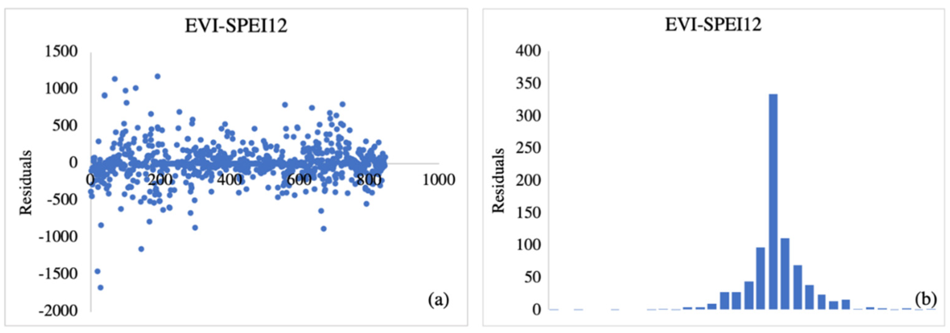
We performed a residual analysis to ensure that the ANN model fit was correct. The residual values were obtained by computing the difference between observed and predicted ANN values. A plot of residuals for all observed and predicted datapoints is illustrated in Figure 3. The randomness of the residual plot (Figure 3a) shows that residuals are independent, while the histogram (Figure 3b) indicates that the random errors inherent in the process were drawn from a normal distribution. These results show that the model fits the data well.
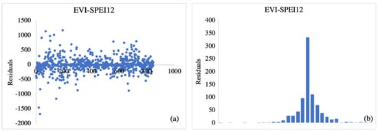
Figure 3.
Plot of ANN crop yield prediction randomness residuals (a) and normal distribution histogram (b).
The results of R2, PBIAS, and MAPE were computed using predicted cotton yields from the 486 ANN model runs of different combinations of DIs and VIs used with CP and CHUs and the corresponding measured data. These results were used to determine the effects of (1) drought and vegetation Indices and (2) dataset size and climate on ANN cotton yield prediction performance and predicted outputs, and to determine (3) how early ANN can provide reasonably accurate cotton yield predictions. However, we summarized the ANN R2 training and testing results to support the findings of the effects of input parameter variables, data size, and climate.
3.1. Effect of Drought and Vegetation Indices Used on ANN Cotton Yield Prediction Outputs and Performance
The ANOVA results of the R2, PBIAS, and MAPE calculated using the predicted cotton yield from the 486 ANN model runs of different combinations of DIs and VIs used with CP and CHUs compared with measured data are summarized in Table 2. Results show that there were no significant differences in mean cotton yield among different combinations of indices and that, in general, the ANN predicted cotton yield fairly well using these readily available inputs. However, there were some significant differences in the mean MAPE, PBIAS, and R2 values among different computation months for drought indices and different combinations of indices. In general, mean MAPE and PBIAS values were within 5%, indicating a very good agreement between mean predicted and observed cotton yield values, with MAPE and PBIAS mean values being highly correlated (correlation coefficient (r) = 0.89). Furthermore, results indicated significant differences in R2 values among different combinations within drought and vegetation indices. In general, drought indices computed at 12 months had significantly higher R2 values, SPEI had higher values than SPI computed at 12 months, and the EVI vegetation index had higher values than LSWI and NDVI when used in combination with SPEI12 (Table 2).
Table 2.
Descriptive statistics and ANOVA results of predicted cotton yield and computed model prediction performance measure values for various CP-CHUs-DI-VI combinations.
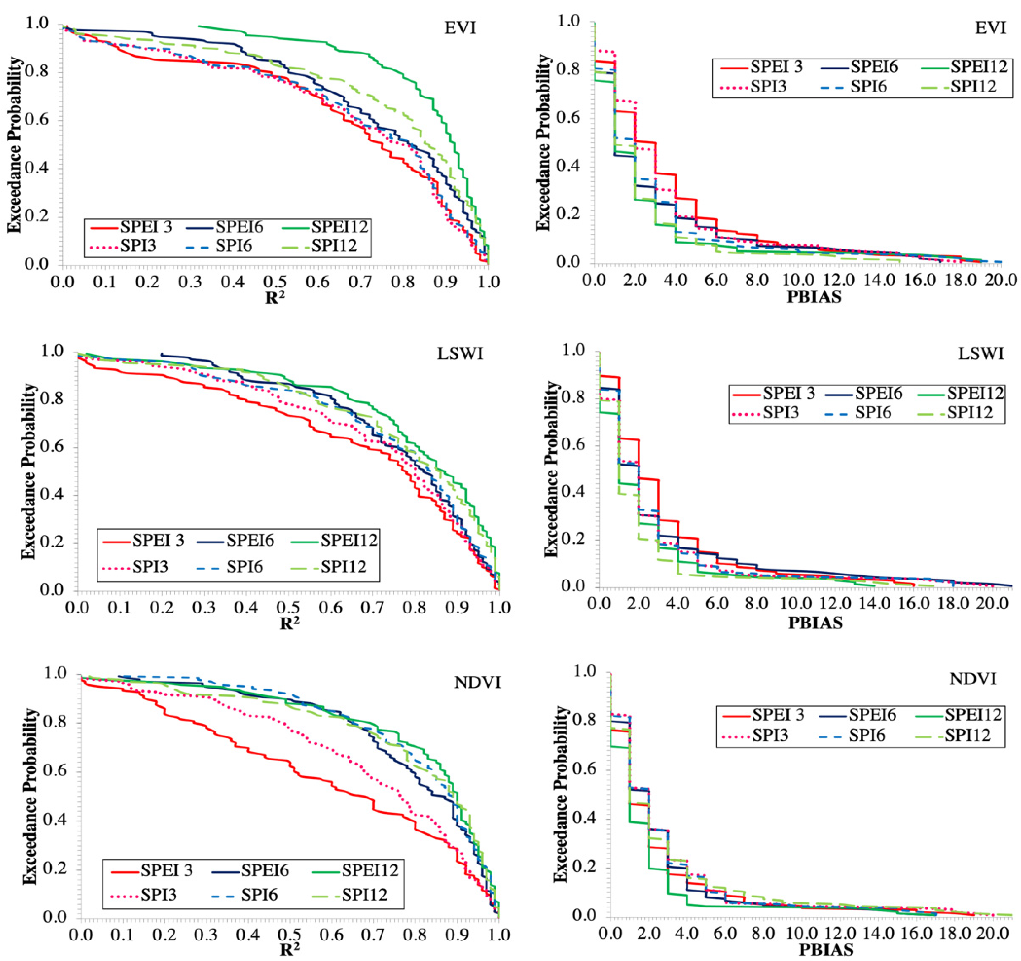
The results of the effects of different combinations of drought and vegetation indices are based on a single mean of 135 data points (27 climate scenarios 5 months). To further validate these findings, the results of the exceedance probability (P) curves for PBIAS and R2 that utilize all 135 data points are presented in Figure 4. The lower the PBIAS and the higher the R2 exceedance p-value, the better the cotton yield prediction. In general, the drought indices computed at 12 months had the lowest PBIAS and highest R2 exceedance p-values, while those computed at three months had the highest PBIAS and lowest R2 exceedance p-values (Figure 4). For example, the probability that a given ANN model run performance would exceed an R2 of 0.70 increased with the length of a monthly interval for drought index calculation with exceedance p-values ranging from 0.49 (NDVI-SPEI3) to 0.60 (EVI-SPI3), 0.60 (EVI-SPI6) to 0.77 (NDVI-SPI6), and 0.71 (EVI-SPI12) to 0.88 (EVI-SPEI12), for drought indices computed at 3, 6, and 12 months, respectively. Conversely, the probability that a given ANN model run performance would exceed PBIAS of 5% decreased with the length of monthly interval with exceedance p-values ranging from 0.26 (NDVI-SPEI3) to 0.13 (EVI-SPEI3), 0.18 (NDVI-SPEI6) to 0.10 (EVI-SPEI6), and 0.18 (EVI-SPI12) to 0.04 (EVI-SPEI12), for drought indices computed at 3, 6, and 12 months, respectively. Between the two drought indices computed at 12 months, SPEI generally had higher exceedance p-values than SPI for R2 > 0.70, with values ranging from 0.77 (LSWI) to 0.88 (EVI) compared with 0.71 (EVI) to 0.76 (NDVI) and lower exceedance p-values than SPI for PBIAS > 5%, with values ranging from 0.10 (LSWI) to 0.04 (EVI) compared with 0.15 (EVI) to 0.05 (LSWI).
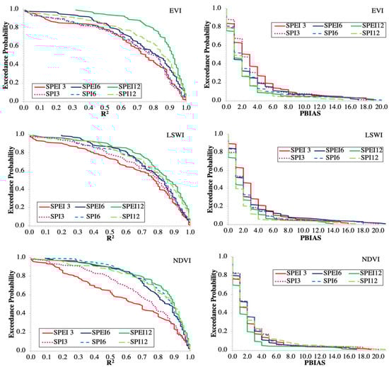
Figure 4.
Exceedance probability curves of computed R2 and PBIAS values for annual cotton yield predicted by ANN using eighteen combinations of drought indices computed at 3, 6, and 12 months and vegetation indices.
Overall, the SPEI12 used with EVI had the lowest PBIAS and highest R2 exceedance p-values, while SPEI3 used with NDVI had the highest PBIAS and lowest R2 exceedance p-values (Figure 4). For example, the EVI-SPEI12 combination had the highest exceedance p-value of 0.88 for the threshold R2 value of 0.70 and the lowest exceedance p-value of 0.04 for PBIAS threshold value of ±5%, while the NDVI-SPEI3 had the lowest exceedance p-value of 0.49 for the threshold R2 value of 0.70 and the highest exceedance p-value of 0.26 for the threshold PBIAS value of ±5%. This implies that 88 % of all (135) EVI-SPEI12-P-HU ANN model runs predicted cotton yield with R2 > 0.70 while 96% of all model runs predicted cotton yield values within 5% of observed cotton yield values. Similarly, 49 % of all (135) NDVI-SPEI3-P-HU ANN model runs predicted cotton yield with R2 > 0.70 while 74% of all model runs predicted cotton yield values within 5% of observed cotton yield values.
The conclusion of EVI-SPEI12 being the superior combination is further supported by R2 training and testing values obtained iteratively during the process of maximizing the prediction ability of the ANN (Table 3). As shown in Table 3, EVI-SPEI12 vegetation index and drought index combination had the best performance as compared with other combinations. The R2 values of training and testing were 0.92 and 0.88, respectively.
Table 3.
The R2 training and testing values of ANN results for various combinations of explanatory variables.
These findings are in agreement with the findings of previous studies. Ref. [79] found that the prediction accuracy of drought improved as the temporal scale at which drought indices (SPI, SPEI) were computed as increased, which they attributed to an increase of the filter length data. This result is in agreement with another previous study indicating increased yield prediction for Spanish cereals’ accuracy using statistical crop models as the time base for SPI calculation increased from one month to three and six months [80]. Other studies have shown that inclusion of evapotranspiration in SPEI improves correlation with crop yield [72,81]. Another study determined that remotely sensed VIs and SPEI could be good tools to predict wheat yield and mitigate yield losses [29]. EVI was found to be a better predictor than NDVI in crop yield estimation using a machine learning model [82]. In addition, Ref. [83] showed that EVI can be used to estimate cotton yield with 91% accuracy. Therefore, EVI, SPEI12, cumulative heat units, and precipitation for months of April, May, June, July, and August were selected and used for the remaining sensitivity analyses in this study. However, the results show that other indices can also be used to predict crop yield, which is supported by previous studies [6,40,79,84,85,86]. For example, Ref. [6] used NDVI and weather data as explanatory variables to predict maize yield in Trans Nzoia and Nakuru County, Kenya with an R2 of 0.86. In another previous study, Kouadio et al. [87] found that both NDVI and EVI performed equally well in predicting spring wheat yield in Canada.
3.2. Effect of Dataset Size and Climate on ANN Cotton Yield Prediction Outputs and Performance
There were no significant differences in mean cotton yield prediction with respect to dataset size (13 vs. 6 years.) and 6-year climate scenarios, except for a significant under-prediction of mean cotton yield during predominantly dry years. The lower predicted cotton yields for the predominantly dry climate scenarios align with the general knowledge that drought decreases rainfed crop yield potential due to water shortage [88,89,90]. The results illustrated that vegetation and hence cotton yield responded to soil water availability and temperature [29,91]. The results of the mean cotton yield predicted by the ANN model and the computed R2 and PBIAS values for each of the 27 dataset sizes (13 vs. 6 years), and twenty six 6-year climate scenarios for each of the five months are presented in Table 4.
Table 4.
Descriptive statistics of ANN cotton yield prediction output and performance for each dataset size and climate scenario category.
Results also indicated that ANN generally predicted cotton yield better using 6-year datasets than 13-year dataset, with significantly lower PBIAS and noticeably higher R2 values, irrespective of climatic condition (Table 4). This result is counterintuitive to the general recommendation in modeling to use as long a dataset as possible [92]. This finding could be attributed to higher probability of ANN to yield good correlation values during the training phase using climatic conditions that are significantly different from the testing phase for the highly variable 13-year than for the 6-year climate scenarios. This explanation is supported by the training and testing R2 values of ANN for different dataset size and climate scenarios presented in Table 5. The training and testing R2 values were relatively within the same ranges for the four 6-year climate scenario categories, while the testing value for the 13-year baseline scenario with greater climate variability was lower (Table 5). Based on the MAPE results, the wet climate scenario has a significantly lower value than the rest of the scenarios. However, although the 13-year baseline scenario resulted in lower R2 and higher MAPE and PBIAS mean values than the 6-year climate scenarios, the ANN predicted cotton yield reasonably well using either 6 or 13-year data and therefore can be used for data-scarce regions.
Table 5.
The R2 training and testing values of ANN results for various dataset size and climate scenarios.
3.3. How Early Can ANN Provide Reasonably Accurate Cotton Yield Predictions?
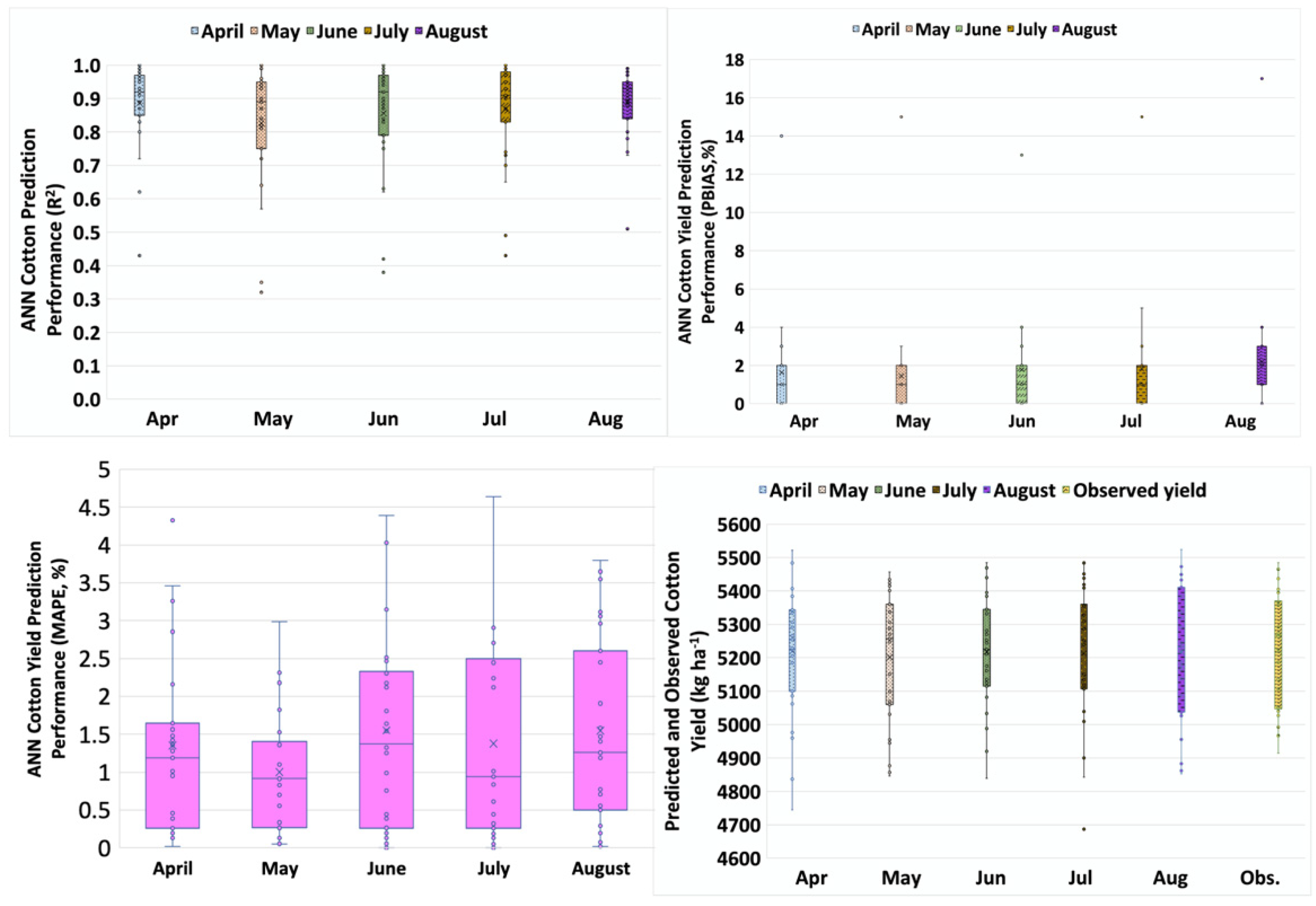
The results of cotton yield predictions using EVI, SPEI12, and CP and CHUs for various months before harvest are presented in Table 6 and Figure 5. Based on these results, there were no significant differences in mean annual cotton yields, computed MAPE, and PBIAS and R2 values using predicted cotton yield for each of the five months (Table 6; Figure 5). This result implies that ANN can be used to accurately predict cotton yield potential as early as April. However, we reasonably conclude that ANN can predict cotton yield potential realistically as early as May since the cotton planting date in April is unknown, with possible planting dates being as late as at the end of the month. Therefore, these results imply that ANN can be used to predict cotton yield potential as early as four months prior to harvest to alert producers about the possible impact of drought on yield.
Table 6.
Descriptive statistic of ANN cotton yield prediction output and performance using EVI, SPEI12, and CP and CHUs for each month.
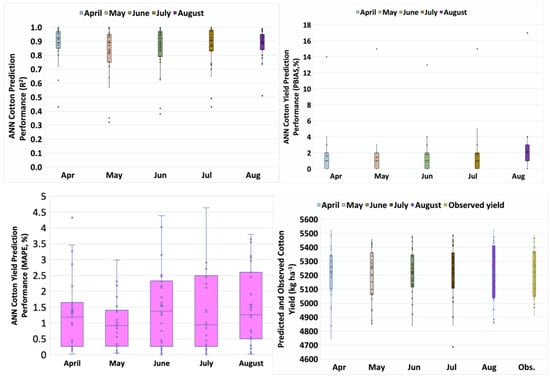
Figure 5.
ANN cotton yield prediction performance and the predicted and observed values.
These results agree with previous studies which reported that satellite-based VIs data from a couple of months prior to harvest can be used for short range crop predictions using statistical regression models [13,93,94]. Other previous studies showed that using VIs with ANN estimated crop yield more 60 days before harvest with high accuracy [95,96,97]. In another previous study, Bouras et al. [98] found that three machine learning models (Support Vector Machine, Random Forest, and eXtreme Gradient Boost) could be used to predict potential yield for three cereals (soft wheat, barley, durum wheat) in Morocco using satellite-based drought indices, weather data, and climate indices four months before harvest. Results showed that the three machine-learning models predicted the yields with RMSE values varying from 0.20 to 0.25 t. ha−1 and R2 values varying from 0.88 to 0.95. Therefore, the ANN model can be used to provide months ahead predictions of cotton yield on the Menemen Plain using variables derived from basic and readily available climate and remotely data. Since cotton is irrigated during the growing season (June-August) in Menemen, the ANN model can inform irrigation water needs based on the cotton yield potential predicted in April and/or May.
Whereas this study focused on the effects of remote sensing DIs and VIs as well datasize and climate on cotton yield prediction, cotton yield is affected by many factors that can be largely categorized as genetics such cotton varieties; environment such as precipitation and temperature; and management practices such as tillage practices, planting date, length of the growing period, fertilizer types, and application rates, and irrigation water management [26,99,100,101,102,103]. Therefore, there is a need for more studies to determine how ANN models can be used to determine the effects of these factors on cotton yield.
4. Conclusions
This study investigated the potential use of ANN for short-range prediction of cotton yield on the Menemen Plain of Turkey as an example data-scarce region using basic and readily available climate and remote sensing input data as explanatory variables. Using drought indices computed at 12-month temporal scales along with VIs, precipitation, and heat units resulted in better cotton yield predictions than drought indices computed at 3- and 6-month temporal scales. In general, SPEI was a better cotton yield predictor than SPI computed at 12 months when used in combination with other described explanatory variables, although all drought and vegetation indices along with precipitation and heat units are generally good cotton yield predictors. Overall, the combination of SPEI computed at 12 months and EVI had the lowest PBIAS and highest R2 values and are, therefore, recommended for this study site. Using these explanatory variables, ANN predicted cotton yield reasonably well using either 6 or 13 year data and can therefore be used for data-scarce regions. Furthermore, results indicated that ANN accurately predicted cotton yield potential as early as April and/or May, which is four to five months before harvest with mean R2 values > 0.8 and MAPE and PBIAS values < 5%. Therefore, the ANN model has the potential to be used by producers as a management tool to provide months ahead predictions of cotton yield on Menemen Plains using variables derived from basic and readily available climate and remotely data. The tool can inform irrigation water needs based on cotton yield potential predicted in April and /or May. Future studies need to focus on how the ANN model can be used to determine how other genetic, environmental, and management related factors affect cotton yield.
Supplementary Materials
The following supporting information can be downloaded at: https://www.mdpi.com/article/10.3390/agronomy12040828/s1, Table S1: The numbers of Landsat 7 ETM images for each month, Table S2: Baseline scenario (BSL) consisting of 13 years with corresponding annual precipitation (P), Table S3: Predominantly 6-year dry climate scenarios (DS) with corresponding annual precipitation (P), Table S4: Predominantly 6-year wet climate scenarios (WS) with corresponding annual precipitation (P), Table S5: Predominantly 6-year average climate scenarios (AS) with corresponding annual precipitation (P), Table S6: Variable climate scenarios (VS) with corresponding annual precipitation (P).
Author Contributions
T.Y.: Conceptualization, Data curation, Formal analysis, Methodology, Software, Validation, Writing—original draft, Writing—review and editing. D.N.M.: Conceptualization, Data curation, Formal analysis, Methodology, Supervision, Validation, Writing—original draft, Writing—review and editing. P.J.S.: Writing—review and editing. D.C.: Writing—review and editing. All authors have read and agreed to the published version of the manuscript.
Funding
This research received no external funding.
Institutional Review Board Statement
Not applicable.
Conflicts of Interest
The authors declare no conflict of interest.
References
- Leo, S.; Migliorati, M.D.A.; Grace, P.R. Predicting within-field cotton yields using publicly available dataset and machine learning. Agron. J. 2020, 113, 1150–1163. [Google Scholar] [CrossRef]
- USDA-FAS (United States Department of Agriculture-Foreign Agricultural Service). Cotton and Products Annual Report: Turkey; United States Department of Agriculture-Foreign Agricultural Service: Washington, DC, USA, 2021; p. 14. Available online: https://apps.fas.usda.gov/newgainapi/api/Report/DownloadReportByFileName?fileName=Cotton%20and%20Products%20Annual_Ankara_Turkey_04-01-2021 (accessed on 15 November 2021).
- IPCC. Food Security. In Climate Change and Land: An IPCC Special Report on Climate Change, Desertification, Land Degradation, Sustainable Land Management, Food Management, Food Security, and Greenhouse Gas Fluxes in Terrestrial Ecosystems 2019; Shukla, P.R., Skea, J., Buendia, E.C., Masson-Delmotte, V., Pörtner, H.-O., Roberts, D.C., Zhai, P., Slade, R., Connors, S., van Diemen, R., et al., Eds.; IPCC: Geneva, Switzerland, 2019; in press. [Google Scholar]
- Zipper, S.C.; Qiu, J.; Kucharik, C.J. Drought effects on US maize and soybean production: Spatiotemporal patterns and historical changes. Environ. Res. Lett. 2016, 11, 094021. [Google Scholar] [CrossRef]
- Dai, A. Increasing drought under global warming in observations and models. Nat. Clim. Change 2013, 3, 52–58. [Google Scholar] [CrossRef]
- Mwaura, J.I.; Kenduiywo, B.K. County level maize yield estimation using artificial neural network. Modeling Earth Syst. Environ. 2020, 7, 1417–1424. [Google Scholar] [CrossRef]
- Lobell, D.B.; Burke, M.B. Satellite detection of rising maize yield heterogeneity in the US Midwest. Env. Res. Lett. 2017, 12, 014014. [Google Scholar] [CrossRef]
- Schmidhuber, J.; Tubiello, F.N. Global food security under climate change. Proc. Natl. Acad. Sci. USA 2007, 104, 19703–19708. [Google Scholar] [CrossRef] [PubMed] [Green Version]
- Filippi, P.; Whelan, B.M.; Vervoort, R.W.; Bishop, T.F.A. Mid-season empirical cotton yield forecasts at fine resolutions using large yield mapping datasets and diverse spatial covariates. Agric. Syst. 2020, 184, 102894. [Google Scholar] [CrossRef]
- Baigorria, G.A.; Chelliah, M.; Mo, K.C.; Romero, C.C.; Jones, J.W.; O’Brien, J.J.; Higgins, R.W. Forecasting cotton yield in the southeastern United States using coupled global circulation models. Agron. J. 2010, 102, 187–196. [Google Scholar] [CrossRef]
- Weiss, M.; Jacob, F.; Duveiller, G. Remote sensing for agricultural applications: A meta-review. Remote Sens. Environ. 2019, 236, 111402. [Google Scholar] [CrossRef]
- Hara, P.; Piekutowska, M.; Niedbala, G. Selection of Independent Variables for Crop Yield Prediction Using Artificial Neural Network Models with Remote Sensing Data. Land 2021, 10, 609. [Google Scholar] [CrossRef]
- Chipanshi, A.; Zhang, Y.; Kouadio, L.; Newlands, N.; Davidson, A.; Hill, H.; Warren, R.; Qian, B.; Daneshfar, B.; Bedard, F.; et al. Evaluation of the Integrated Canadian Crop Yield Forecaster (ICCYF) model for in-season prediction of cro yield across the Canadian agricultural landscape. Agric. For. Meteorol. 2015, 206, 137–150. [Google Scholar] [CrossRef] [Green Version]
- Ali, M.; Deo, R.C.; Downs, N.J.; Maraseni, T. Cotton yield prediction with Markov Chain Monte Carlo-based simulation model integrated with genetic programing algorithm: A new hybrid copula-driven approach. Agric. For. Meteorol. 2018, 263, 428–448. [Google Scholar] [CrossRef]
- Ali, M.; Deo, R.C.; Downs, N.J.; Maraseni, T. An ensemble-ANFIS based uncertainty assessment model for forecasting multi-scalar standardized precipitation index. Atmos. Res. 2018, 207, 155–180. [Google Scholar] [CrossRef]
- Ali, M.; Deo, R.C.; Downs, N.J.; Maraseni, T. Multi-stage hybridized online sequential extreme learning machine integrated with Markov Chain Monte Carlo copula-Bat algorithm for rainfall forecasting. Atmos. Res. 2018, 213, 450–464. [Google Scholar] [CrossRef]
- Bauer, M.E. The role of remote sensing in determining the distribution and yield of crops. Adv. Agron. 1975, 27, 271–304. [Google Scholar]
- Nguyen-Huy, R.; Deo, R.C.; An-Vo, D.A.; Mushtaq, S.; Khan, S. Copula-statistical precipitation forecasting model in Australia’s agro-ecological zones. Agric. Water Manag. 2017, 191, 153–172. [Google Scholar] [CrossRef]
- Soh, Y.W.; Koo, C.H.; Huang, Y.F.; Fung, K.F. Application of artificial intelligence models for the prediction of standardized precipitation evapotranspiration index (SPEI) at Langat River Basin, Malaysia. Comput. Electron. Agric. 2018, 144, 164–173. [Google Scholar] [CrossRef]
- Djerbouai, S.; Souag-Gamane, D. Drought forecasting using neural networks, wa- velet neural networks, and stochastic models: Case of the Algerois Basin in North Algeria. Water Resour. Manag. 2016, 30, 2445–2464. [Google Scholar] [CrossRef]
- Tsangaratos, P.; Ilia, I. Comparison of a logistic regression and NaA ve Bayes classifies in landslide susceptibility assessments: The influence of models complexity and training dataset size. CATENA 2016, 145, 164–179. [Google Scholar] [CrossRef]
- Gupta, H.V.; Sorooshian, S.; Yapo, P.O. Status of automatic calibration for hydrologic models: Comparison with multilevel expert calibration. J. Hydrol. Eng. 1999, 4, 135–143. [Google Scholar] [CrossRef]
- Aslam, S.; Khan, S.H.; Ahmed, A.; Dandekar, A.M. The tale of cotton plant: From wild type to domestication, leading to its improvement by genetic transformation. Am. J. Mol. Biol. 2020, 10, 91–127. [Google Scholar] [CrossRef] [Green Version]
- Turkish Ministry of Trade (TMT). Cotton Report of 2018; Turkish Ministry of Trade (TMT): Ankara, Turkey, 2018. Available online: http://ticaret.gov.tr/data/5d41e59913b87639ac9e02e8/d0e2b9c79234684as29baf256a0e7dce.pdf (accessed on 13 August 2021).
- Guo, W.; Maas, S.J.; Bronson, K.F. Relationship between cotton yield and soil electrical conductivity, topography, and Landsat imagery. Precis. Agric. 2012, 13, 678–692. [Google Scholar] [CrossRef]
- Sawan, Z.M. Cotton production and climatic factors: Studying the nature of its relationship by different statistical methods. Cogent Biol. 2017, 3, 1292882. [Google Scholar] [CrossRef]
- Mauget, S.; Ulloa, M.; Dever, J. Planting data effects on cotton lint yield and fiber quality in the US Southern High Plains. Agriculture 2019, 9, 82. [Google Scholar] [CrossRef] [Green Version]
- Yang, M.; Mou, Y.; Meng, Y.; Liu, S.; Peng, C.; Zhou, X. Modeling the effects of precipitation and temperature patterns on agricultural drought in China from 1949 to 2015. Sci. Total Environ. 2020, 711, 135139. [Google Scholar] [CrossRef] [PubMed]
- Feng, P.; Wang, B.; Liu, D.L.; Yu, Q. Machine learning-based integration of remotely-sensed drought factors can improve the estimation of agricultural drought in South-Eastern Australia. Agric. Syst. 2019, 173, 303–316. [Google Scholar] [CrossRef]
- Zuo, D.; Cai, S.; Xu, Z.; Peng, D.; Kan, G.; Sun, W.; Pang, B.; Yang, H. Assessment of meteorological and agricultural droughts using in-situ observations and remote sensing data. Agric. Water Manag. 2019, 222, 125–128. [Google Scholar] [CrossRef]
- Park, S.J.; Hwang, C.S.; Vlek, P.L.G. Comparison of adaptive techniques to predict crop yield response under varying soil and land management conditions. Agric. Syst. 2005, 85, 59–81. [Google Scholar] [CrossRef]
- Masasi, B.; Taghvaenian, S.; Gowda, P.H.; Moriasi, D.N.; Starks, P.J. Assessment of heat unit availability and potential lint yield of cotton in Oklahoma. Appl. Eng. Agric. 2020, 36, 943–954. [Google Scholar] [CrossRef]
- Glade, E.H., Jr.; Meyer, L.; Stults, H. The Cotton Industry in the United States; Agricultural Economic Report; Economic Research Service, USDA: Washington, DC, USA, 1996. [Google Scholar]
- Killi, F.; Bolek, Y. Timing of planting is crucial for cotton yield. Acta Agric. Scand. 2004, 56, 155–160. [Google Scholar] [CrossRef]
- Karl, T.R.; Koscielny, A.J. Drought in the United States: 1895–1981. J. Climatol. 1982, 2, 313–329. [Google Scholar] [CrossRef]
- Yamoah, C.F.; Walters, D.T.; Shapiro, C.A.; Francis, C.A.; Hayes, M.J. Standardized Precipitation Index and nitrogen rate effects on crop yields and risk distribution in maize. Agric. Ecosyst. Environ. 2000, 80, 113–120. [Google Scholar] [CrossRef]
- Quiring, S.M.; Papakryiakou, T.N. An evaluation of agricultural drought indices for the Canadian prairies. Agric. For. Meteorol. 2003, 118, 49–62. [Google Scholar] [CrossRef]
- Kaul, M.; Hill, R.L.; Walthall, C. Artificial neural networks for corn and soybean yield prediction. Agric. Syst. 2005, 85, 1–18. [Google Scholar] [CrossRef]
- Feng, P.; Wang, B.; Liu, D.L.; Waters, C.; Xiao, D.; Shi, L.; Yu, Q. Dynamic wheat yield forecasts are improved by a hybrid approach using a biophysical model and machine learning technique. Agric. For. Meteorol. 2020, 285–286, 107922. [Google Scholar] [CrossRef]
- McKee, T.B.; Doesken, N.J.; Kleist, J. The relationship of drought frequency and duration to time scales. In Proceedings of the Eighth Conference on Applied Climatology, Anaheim, CA, USA, 17–22 January 1993; pp. 179–184. [Google Scholar]
- Vicente-Serrano, S.M.; Beguería, S.; López-Moreno, J.I. A multiscalar drought index sensitive to global warming: The standardized precipitation evapotranspiration index. J. Clim. 2010, 23, 1696–1718. [Google Scholar] [CrossRef] [Green Version]
- Xiao, X.; Zhang, Q.; Saleska, S.; Hutyra, L.; Camargo, P.D.; Wofsy, S.; Frolking, S.; Boles, S.; Keller, M.; Moore, B. Satellite-based modeling of gross primary production in a seasonally moist tropical evergreen forest. Remote Sens. Environ. Vol. 2005, 94, 105–122. [Google Scholar] [CrossRef]
- Huete, A.; Didan, K.; Miura, T.; Rodriguez, E.P.; Gao, X.; Ferreira, L.G. Overview of the radiometric and biophysical performance of the MODIS vegetation indices. Remote Sens. Environ. 2002, 83, 195–213. [Google Scholar] [CrossRef]
- Xiao, X.; Braswell, B.; Zhang, Q.; Boles, S.; Frolking, S.; Moore, B. Sensitivity of vegetation indices to atmospheric aerosols: Continental-scale observations in Northern Asia. Remote Sens. Environ. 2003, 84, 385–392. [Google Scholar] [CrossRef]
- Huete, A.R.; Justice, C.; Van Leeuwen, W. MODIS Vegetation Index (MOD13). Algorithm Theoretical Basis Document (ATBD) 1999, Version 3. Available online: https://modis.gsfc.nasa.gov/data/atbd/atbd_mod13.pdf (accessed on 3 January 2022).
- Chakraborty, K. Vegetation change detection in Barak Basin. Curr. Sci. 2009, 96, 1236–1242. [Google Scholar]
- Setiawan, Y.; Yoshino, K. Temporal pattern analysis of wavelet-filtered MODIS EVI to detect land use change in JAVA island, Indonesia. Int. Arch. Photogramm. Remote Sens. Spat. Inf. Sci. 2010, 38, 820–825. [Google Scholar]
- Priyadarshi, N.; Chowdary, M.; Srivastava, Y.; Das, I.C.; Jha, C.S. Reconstruction of time series MODIS EVI data using de-nosing algorithms. Geocarto Int. 2017, 33, 1095–1113. [Google Scholar] [CrossRef]
- Zhang, X.; Wu, B.; Ponce-Campos, G.E.; Zhang, M.; Chang, S.; Tian, F. Mapping up-to-Date Paddy Rice Extent at 10 M Resolution in China through the Integration of Optical and Synthetic Aperture Radar Images. Remote Sens. 2018, 10, 1200. [Google Scholar] [CrossRef] [Green Version]
- Huete, A.R.; Liu, H.Q.; Batchily, K.; Van Leeuwen, W. A comparison of vegetation indices global set of TM images for EOS-MODIS. Remote Sens. Environ. 1997, 59, 440–451. [Google Scholar] [CrossRef]
- Gao, B.C. NDWI—A normalized difference water index for remote sensing of vegetation liquid water from space. Remote Sens. Environ. 1996, 58, 257–266. [Google Scholar] [CrossRef]
- Hereher, M.E. Environmental monitoring and change assessment of Toshka lakkes in southern Egypt using remote sensing. Environ. Earth Sci. 2015, 73, 3623–3632. [Google Scholar] [CrossRef]
- Chandrasekar, K.; Sesha Sai, M.; Roy, P.; Dwevedi, R. Land surface water index (LSWI) response to rainfall and NDVI using the MODIS vegetation index product. Int. J. Remote Sens. 2010, 31, 3987–4005. [Google Scholar] [CrossRef]
- Ma, S.; Zhou, Y.; Gowda, P.H.; Dong, J.; Zhang, G.; Kakani, V.G.; Wagle, P.; Chen, L.; Flynn, K.C.; Jiang, W. Application of the water-related spectral reflectance indices: A review. Ecol. Indic. 2019, 98, 68–79. [Google Scholar] [CrossRef]
- Chen, D.; Huang, J.; Jackson, T.J. Vegetation water content estimation for corn and soybeans using spectral indices derived from MODIS near and short-wave infrared bands. Remote Sens. Environ. 2005, 98, 225–236. [Google Scholar] [CrossRef]
- Jackson, T.J.; Chen, D.; Cosh, M.; Li, F.; Anderson, M.; Walthall, C.; Doriaswamy, P.; Hunt, E.R. Vegetation water content mapping using Landsat data derived normalized difference water index for corn and soybeans. Remote Sens. Environ. 2004, 92, 475–482. [Google Scholar] [CrossRef]
- Ozturk, M.Z.; Cetinkaya, G.; Aydin, S. Climate types of Turkey according to Koppen-Geiger climate classification. Istanb. Univ. J. Geogr. 2017, 35, 17–27. [Google Scholar]
- Korkmaz, N. Determining the Water Distribution Performance and Irrigation Efficiencies on Farm Level in Menemen Left Bank Irrigation System. Ph.D. Thesis, Ege University, Bornova, Turkey, 2008. [Google Scholar]
- Turkish State Meteorological Service (TSMS). Report (Personal communication); Turkish State Meteorological Service (TSMS): Ankara, Turkey, 2020.
- Eryuce, N.; Ozkan, C.F.; Anac, D.; Asri, F.Ö.; Güven, D.; Demirtas, E.L.; Simsek, M.; Ari, N. Effect of different potassium fertilizers on cotton yield and quality in Turkey. Int. Fertil. Corresp. (e-ifc) 2019, 12–20. Available online: https://www.ipipotash.org/publications/effect-of-potassium-fertilizers-on-cotton-yield-quality-turkey (accessed on 23 February 2022).
- Turkish Statistical Institute (TSI.; TUIK). Crop Production Statistics. 2020. Available online: https://biruni.tuik.gov.tr/medas/?kn=92&locale=tr (accessed on 11 November 2021).
- Guttman, N.B. Accepting the Standardized Precipitation Index: A Calculation Algorithm. J. Am. Water Resour. Assoc. 1999, 35, 311–322. [Google Scholar] [CrossRef]
- Lloyd-Hughes, B.; Saunders, M.A. A drought climatology for Europe. Int. J. Clim. 2002, 22, 1571–1592. [Google Scholar] [CrossRef]
- Livada, I.; Assimakopoulos, V.D. Spatial and temporal analysis of drought in Greece using the Stardardized Precipitation Index (SPI). Theor. Appl. Climatol. 2007, 89, 143–153. [Google Scholar] [CrossRef]
- Hargreaves, G.H.; Samani, Z.A. Reference crop evapotranspiration from ambient air temperature. Appl. Eng. Agric. 1985, 1, 96–99. [Google Scholar] [CrossRef]
- Allen, R.; Pereira, L.; Raes, D.; Smith, M. Crop Evapotranspiration; FAO Irrigation and Drainage Paper 56; FAO: Rome, Italy, 1998; p. 164. [Google Scholar]
- Tan, C.P.; Yang, J.P.; Li, M. Temporal-spatial variation of drought indicated by SPI and SPEI in Ningxia Hui autonomous region, China. Atmosphere 2015, 6, 1399–1421. [Google Scholar] [CrossRef] [Green Version]
- Tucker, C.J. Red and photographic infrared linear combinations for monitoring vegetation. Remote Sens. Environ. 1979, 8, 127–150. [Google Scholar] [CrossRef] [Green Version]
- Jiang, Z.; Huete, A.R.; Didan, K.; Miura, T. Development of a two-band enhanced vegetation index without a blue band. Remote Sens. Environ. 2008, 112, 3833–3845. [Google Scholar] [CrossRef]
- Xiao, X.; Boles, S.; Frolking, S.; Salas, W.; Moore, B., III; Li, C.; He, L.; Zhao, R. Observation of flooding and rice transplanting of paddy rice fields at the site to landscape scales in China using VEGETATION sensor data. Int. J. Remote Sens. 2002, 23, 3009–3022. [Google Scholar] [CrossRef]
- Davidonis, G.H.; Johnson, A.S.; Landivar, J.A.; Fernandez, C.J. Cotton fiber quality is related to boll location and planting date. Agron. J. 2004, 96, 42–47. [Google Scholar] [CrossRef]
- Starks, P.J.; Steiner, J.L.; Neel, J.P.S.; Turner, K.E.; Northup, B.K.; Gowda, P.H.; Brown, M.A. Assessment of the Standardized Precipitation and Evaporation Index (SPEI) as a Potential Management Tool for Grasslands. Agronomy 2019, 9, 235. [Google Scholar] [CrossRef] [Green Version]
- Lawrence, J. Introduction to Neural Networks: Design, Theory, and Applications 1994, 6th ed.; California Scientific Software: Nevada City, CA, USA, 1994. [Google Scholar]
- Yang, T.; Asanjan, A.A.; Welles, E.; Gao, X.; Sorooshian, S.; Liu, X. Developing reservoir monthly inflow forecasts using artificial intelligence and climate phenomenon information. Water Resour. Res. 2017, 53, 2786–2812. [Google Scholar] [CrossRef]
- Ballabio, D.; Vasighi, M.A. MATLAB toolbox for Self Organizing Maps and supervised neural network learning strategies. Chemom. Intell. Lab. Syst. 2012, 118, 24–32. [Google Scholar] [CrossRef]
- Panchal, G.; Ganatra, A.; Kosta, Y.P.; Panchal, D. Behaviour Analysis of Multilayer Perceptrons with Multiple Hidden Neurons and Hidden Layers. Int. J. Comput. Theory Eng. 2011, 3, 332–337. [Google Scholar] [CrossRef] [Green Version]
- Mercioni, M.A.; Tiron, A.; Holban, S. Dynamic modification of activation function using the backpropagation algorithm in the artificial neural networks. Int. J. Adv. Comput. Sci. Appl. 2019, 10, 51–56. [Google Scholar] [CrossRef]
- Mia, M.; Khan, M.A.; Dhar, N.R. Study of surface roughness and cutting forces using ANN, RSM, and ANOVA in turning of Ti-6Al-4V under cryogenic jets applied at flank and rake faces of coated WC tool. Int. J. Adv. Manuf. Technol. 2017, 93, 975–991. [Google Scholar] [CrossRef]
- Zhang, R.; Chen, Z.Y.; Xu, L.J.; Ou, C.Q. Meteorological drought forecasting based on a statistical model with machine learning techniques in Shaanxi province, China. Sci. Total Environ. 2019, 665, 338–346. [Google Scholar] [CrossRef]
- García-Leóna, D.; Contrerasc, S.; Hunink, J. Comparison of meteorological and satellite-based drought indices as yield predictors of Spanish cereals. Agric. Water Manag. 2019, 213, 388–396. [Google Scholar] [CrossRef]
- Labudova, L.; Labuda, M.; Takac, J. Comparison of SPI and SPEI applicability for drought impact assessment on crop production in the Danubian Lowland and the East Slovakian Lowland. Appl. Clim. 2017, 128, 491–506. [Google Scholar] [CrossRef]
- Johnson, M.D.; Hsieh, W.W.; Cannon, A.J.; Davidson, A.; Bedard, F. Crop yield forecasting on the Canadian Prairies by remotely sensed vegetation indices and machine learning methods. Agric. For. Meteorol. 2016, 218–219, 74–84. [Google Scholar] [CrossRef]
- Liu, Q.S.; Li, X.Y.; Liu, G.H.; Huang, C.; Guo, Y.S. Cotton area and yield estimation at Zhanhua County of China using HJ-1 EVI time series. ITM Web Conf. 2016, 7, 09001. [Google Scholar] [CrossRef]
- Vicente-Serrano, S.; Cuadrat-Prats, J.M.; Romos, A. Early prediction of crop production using drought indices at different time-scales and remote sensing data: Application in Ebro Valley (north-east Spain). Int. J. Remote Sens. 2006, 27, 511–518. [Google Scholar] [CrossRef]
- Törnros, T.; Menzel, L. Addressing drought conditions under current and future climate in the Jordan River region. Hydrol. Earth Syst. Sci. 2014, 18, 305–318. [Google Scholar] [CrossRef] [Green Version]
- Pena-Gallardo, M.; Vicente-Serrano, S.M.; Quiring, S.; Svoboda, M.; Hannaford, J.; Tomas-Burguera, M.; Martin-Hernandez, N.; Dominguez-Castro, F.; El Kenawy, A. Response of crop yield to different time-scales of drought in the United States: Spatio-temporal patterns and climatic and environmental drivers. Agric. For. Meteorol. 2019, 264, 40–55. [Google Scholar] [CrossRef] [Green Version]
- Kouadio, L.; Newlands, N.K.; Davidson, A.; Zhang, Y.; Chipanshi, A. Assessing the performance of MODIS NDVI and EVI for seasonal crop yield forecasting at the ecodistrict scale. Remote Sens. 2014, 6, 10193–10214. [Google Scholar] [CrossRef] [Green Version]
- Kuwayama, Y.; Thompson, A.; Bernknopf, R.; Zaitchik, B.; Vail, P. Estimating the Impact of Drought on Agriculture Using the US Drought Monitor. Am. J. Agric. Econ. 2018, 101, 193–210. [Google Scholar] [CrossRef]
- Ray, R.L.; Fares, A.; Risch, E. Effects of drought on crop production and cropping areas in Texas. Agric. Environ. Lett. 2018, 3, 1–15. [Google Scholar] [CrossRef] [Green Version]
- Leng, G.; Hall, J. Crop yield sensitivity of global major agricultural countries to drought and the projected changes in the future. Sci. Total Environ. 2019, 654, 811–821. [Google Scholar] [CrossRef] [PubMed]
- Park, S.; Im, J.; Jang, E.; Rhee, J. Drought assessment and monitoring through blending of multi-sensor indices using machine learning approaches for different climate regions. Agric. For. Meteorol. 2016, 216, 157–169. [Google Scholar] [CrossRef]
- Nelson, A.M.; Moriasi, D.N.; Talebizadeh, M.; Steiner, J.L.; Confesor, R.; Gowda, P.H.; Starks, P.J.; Tadesse, H. Impact of length of dataset on streamflow calibration parameters and model performance. J. Am. Water Resour. Assoc. (JAWRA) 2017, 53, 1164–1177. [Google Scholar] [CrossRef]
- Mkhabela, M.S.; Bullock, P.; Raj, S.; Yang, Y. Crop yield forecasting on the Canadian Prairies using MODIS NDVI data. Agric. For. Meteorol. 2011, 151, 385–393. [Google Scholar] [CrossRef]
- Seiler, R.A.; Kogan, F.; Wei, G. Monitoring weather impact and crop yield from NOAA AVHRR data in Argentina. Adv. Space Res. 2000, 26, 1177–1185. [Google Scholar] [CrossRef]
- Khaki, S.; Pham, H.; Wang, L. Yieldnet: A convolutional neural network for simultaneous corn and soybean yield prediction based on remote sensing data. Sci. Rep. 2021, 11, 11132. [Google Scholar] [CrossRef] [PubMed]
- Alvarez, R. Predicting average regional yield and production of wheat in the Argentine Pampas by an artificial neural network approach. Eur. J. Agron. 2009, 30, 70–77. [Google Scholar] [CrossRef]
- Li, A.; Liang, S.; Wang, A.; Qin, J. Estimating crop yield from Multi-temporal satellite data using multivariate regression and neural network techniques. Photogramm. Eng. Remote Sens. 2007, 73, 1149–1157. [Google Scholar] [CrossRef] [Green Version]
- Bouras, E.H.; Jarlan, L.; Er-Raki, S.; Balaghi, R.; Amazirh, A.; Richard, B.; Khabba, S. Cereal yield forecasting with satellite drought-based indices, weather data and regional climate indices using machine learning in Morocco. Remote Sens. 2021, 13, 3101. [Google Scholar] [CrossRef]
- Bakhsh, K.; Hassan, I.; Maqbool, A. Factors affecting cotton yield: A case study of Sargodha (Pakistan). J. Agric. Soc. Sci. 2005, 1, 332–334. [Google Scholar]
- Chaudhry, I.S.; Khan, M.B. Factors affecting cotton production in Pakistan: Empirical evidence from Multan District. J. Qual. Technol. Manag. 2009, 5, 91–100. [Google Scholar]
- Haghverdi, A.; Washington-Allen, R.A.; Leib, B.G. Prediction of cotton lint yield from phenology of crop indices using artificial neural networks. Comput. Electron. Agric. 2018, 152, 186–197. [Google Scholar] [CrossRef]
- Pokhrel, B.K.; Paudel, K.P.; Segarra, E. Factors affecting the choice, intensity, and allocation of irrigation technologies by U.S. cotton farmers. Water 2018, 10, 706. [Google Scholar] [CrossRef] [Green Version]
- Niedbala, G. Application of artificial neural networks for multi-criteria yield prediction of winter rapeseed. Sustainability 2019, 11, 533. [Google Scholar] [CrossRef] [Green Version]
Publisher’s Note: MDPI stays neutral with regard to jurisdictional claims in published maps and institutional affiliations. |
© 2022 by the authors. Licensee MDPI, Basel, Switzerland. This article is an open access article distributed under the terms and conditions of the Creative Commons Attribution (CC BY) license (https://creativecommons.org/licenses/by/4.0/).