Peak Shift of Coherent Edge Radiation Spectrum Depending on Radio Frequency Field Phase of Accelerator

Abstract

Spectra of coherent edge radiation (CER) were observed at the S-band linac facility of Kyoto University Free Electron Laser. A local maximum was observed in the CER spectrum on-crest operation of the radio frequency (RF) field. As the phase of the RF field was shifted from the crest, the frequency of the maximum decreased, and the CER spectrum approached a spectrum of Gaussian-distributed electrons in a bunch. It was found that this strange spectrum can be explained by a model in which a satellite pulse exists around a main pulse in the electron bunch. Furthermore, it demonstrated that CER is an effective tool for monitoring the shape of the electron bunch.

1. Introduction

Coherent radiation emitted by relativistic electrons is not only used for spectroscopic measurements and imaging experiments as a high-intensity light source [1,2,3] but is also an effective tool for evaluating the shape of an electron bunch. In particular, because the bunch length is 1 mm or less in S-band linacs, high-intensity coherent radiation is generated in the frequency range of sub-terahertz to terahertz (THz), where the electromagnetic waves can be used optically [4]. Transporting the coherent radiation from a light source to detectors is relatively simple; moreover, it can be measured quantitatively. Several studies have been conducted on the electron bunch shape using various types of coherent radiation [5,6,7,8]. Coherent edge radiation (CER) propagates on the conical surface and can be extracted and used simultaneously with other light sources [9,10]. Recently, a phenomenon whereby the CER intensity was amplified on oscillation of a free-electron laser (FEL) was discovered [11]. It is expected that this phenomenon would elucidate the complete picture of the change of the electron bunch shape due to the FEL interaction by observing the CER.

Subsequently, we constructed a measurement system for the CER generated at the downstream bending magnet of the undulator straight section at Kyoto University Free Electron Laser (KU-FEL) [12]. The CER beam was extracted from the FEL cavity by inserting a flat mirror in front of the downstream cavity mirror, and the electron bunch shape was evaluated from the CER spectrum when FELs did not oscillate. In our previous study [12], we reported that the electron bunch had a Gaussian distribution in operations with an electron energy of 30 MeV or less. When the electron energy was increased to 40 MeV, it was observed that a strange maximum appeared in the spectrum of CER. When a phase of the accelerator tube was shifted from the crest of the RF field, the maximum moved to the low frequency side, and the spectrum had become similar to that for an electron bunch with Gaussian distribution. Such a spectrum with a maximum suggested the presence of a dip in the electron bunch shape. It was found that the observed spectrum could be explained when the electron bunch comprised a main pulse and small satellite pulse. In this paper, we discuss the strange CER spectrum observed at KU-FEL and the satellite pulse model for the electron bunch shape.

2. Materials and Methods

2.1. Infrared FEL Facility KU-FEL

As shown in Figure 1, the infrared FEL facility KU-FEL is based on a normal conducting S-band linac with a thermionic radio frequency (RF) gun as the electron source [13]. A multi-bunch electron beam with an energy of 8.4 MeV was generated in the thermionic RF gun driven by a 10 MW klystron. After passing through a dog-leg type energy filter, the electron beam is injected into a 3 m accelerator tube driven by a 20-MW klystron. The electron beam bunches were compressed by passing them through a 180° arc section and were injected into a 1.8 m hybrid planar undulator with a period of 33 mm for the FEL oscillations. An optical cavity with a length of 5.039 m is installed on the extension of the undulator straight line [14]. The maximum energy of an electron is 40 MeV, and the duration of the electron beam macropulse can be up to 7.8 μs. Although the charge of the electron beam micropulse increases from 20 to 50 pC owing to the back-bombardment effects on the thermionic RF gun, the electron energy of the micropulse is kept constant during the macropulse duration by applying amplitude-modulated RF pulses to the RF gun and accelerator tube [15]. In this experiment, the electron beam was operated under the electron energy of 40 MeV and macropulse duration of 6.9 μs. The K value of the undulator was set to 1.28, and the wavelength of FEL oscillations was 4.9 μm.

The FEL power was varied by adjusting the phase of the RF field between the RF gun and the accelerator tube. Figure 2 shows the FEL macropulse for some RF phase differences. Here, the RF phase difference on the crest was defined as zero. As shown in Figure 2, the FEL power was maximized near the crest and the maximum value was approximately 40 mJ. Therefore, the bunch length of the electron beam was expected to be minimal near the crest.

2.2. Observation System for CER Spectrum

The outline of the observation system for the CER is shown in Figure 1 [12]. The CER beam is extracted from the optical cavity by inserting a flat mirror tilted at an angle of 45° to the optical axis in the horizontal plane. The distance from the light source of the downstream bending magnet to the flat mirror was 0.56 m. The effective area of the deflection mirror projected onto the plane perpendicular to the optical axis was 20 mm². The electron beam generated CER at both the ends of the undulator, the exit of the upstream bending magnet, and the entrance of the downstream bending magnet in the undulator straight section. However, the magnetic field at the end of the undulator was significantly lower than that at the bending magnet, and the CER generated at the undulator was negligible compared to that generated at the bending magnet [16]. The CER generated at the upstream bending magnet was reflected to the inner surface of the vacuum chamber of the undulator multiple times; therefore, it did not reach the flat mirror while maintaining coherence. Therefore, only the CER beam generated at the downstream bending magnet was extracted to the atmosphere through a vacuum window made of z-cut crystal quartz with a thickness of 4 mm. The extracted CER beam was deflected by a concave mirror with a diameter of 76 mm and radius of curvature of 1 m positioned at 0.8 m from the radiation point and was transported to a Michelson interferometer. A nitrocellulose pellicle with a thickness and diameter of 2 μm and 76 mm, respectively, identical to that of the beam splitter used for the Michelson interferometer, was inserted between the concave mirror and Michelson interferometer. The pellicle was coated by a nickel-based alloy, and the transmittance and reflectance in the THz region were approximately 60% and 10%, respectively [12]. The component reflected by the pellicle is used as reference light. A movable mirror with a diameter of 50 mm was employed to manipulate the optical path difference of the interferometer by up to 100 mm. The autocorrelation signal was concentrated by a parabolic mirror with a focal length of 76 mm and diameter of 51 mm and measured using a pyroelectric energy meter (Sensor-und Lasertechnik Inc. (Wildau, Germany), THz10) with a sensor diameter of 10 mm. A black polyethylene film with a thickness of 60 μm was installed in front of the energy meter to suppress the unwanted infrared radiation. The reference light was also measured by separate pyroelectric energy meter with a different black polyethylene film.

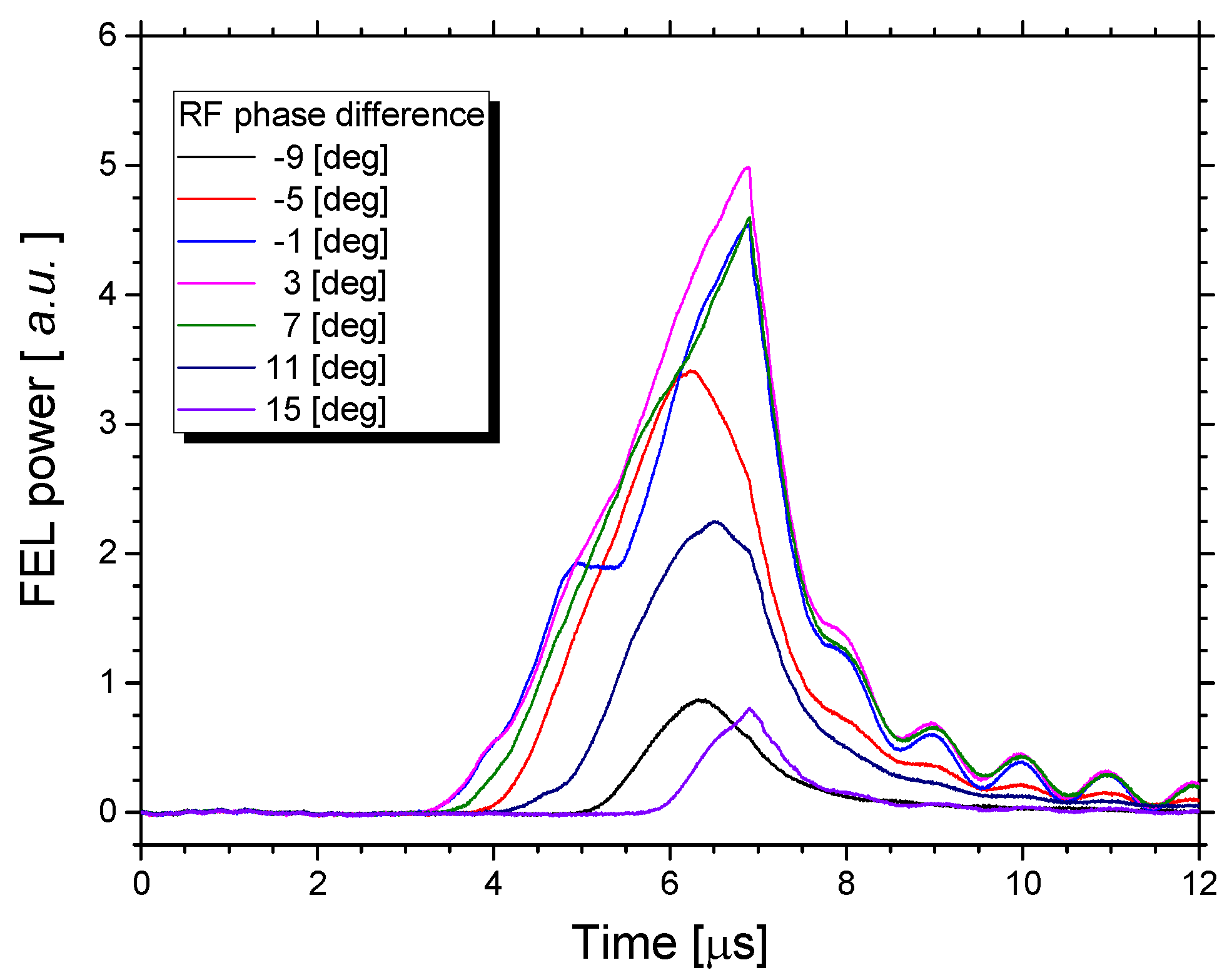
2.3. Characteristics of the Measured CER Spectra

The CER spectra were measured with the observation system by changing the RF phase between the RF gun and accelerator tube. The movable mirror of the interferometer was scanned at a step interval of 10 μm in a length of ±0.3 mm around the zero optical path length. The signal was measured four times for one position and the average values were used as the power of the interferometer. The relative standard deviation of the averaged signals was only 0.64%. Figure 3a shows the measured CER spectra for some RF phase differences. As the spectral measurements were performed in air, dips appeared owing to the absorption of water vapor at the frequencies of 0.56, 0.75, 0.99, 1.1–1.3, 1.4, and 1.6–1.7 THz in the CER spectra [17]. The CER spectra rapidly decreased below 0.2 THz. This decrease was caused by a diffraction loss of the optical system for the CER beam [18]. In this experiment, the cutoff frequency f_c of the diffraction loss was as high as 0.2 THz owing to the misalignment of the detector [12]. As shown in Figure 3a, the intensity of the CER beam was maximized at the RF phase difference near the crest, and the maximum of the CER spectrum on the crest appeared at a frequency of 0.6 THz. The high frequency component of the CER spectrum decreased as the RF phase difference ∆ increased in the region of ∆ > 0, and the CER spectrum at ∆ = 15° closed to the previously reported CER spectrum when the electrons in the bunch were Gaussian distribution [12].

Therefore, assuming that the electron bunch shape was the Gaussian distribution, we evaluated the bunch length based on the measured spectrum at ∆ = +15°. The CER spectrum irradiated on the flat mirror, U_CER(ω), and the observed CER spectrum, O(ω), had the following relationship:

$$O\left(\omega \right)=\left[1-{\mathrm{e}}^{-{\left(\frac{\omega }{2\pi f_c}\right)}^2}\right]S\left(\omega \right)T\left(\omega \right)U_{\mathit{CER}}\left(\omega \right)$$

(1)

where S(ω) and T(ω) are the sensitivity of the detector and transmittance of the optical transport system, respectively [12]. The pyroelectric energy meter used in the experiment had a flat sensitivity in the frequency range of 0.3–3 THz where the CER beam was not affected by the diffraction loss. Therefore, the effect of S(ω) on the observed CER spectrum is negligible. In addition to absorption by water vapor, it is necessary to consider the z-cut crystal quartz window and the black polyethylene film for the transmittance of the optical transport system. The crystal quartz has a substantially constant transmittance of 0.78 in the frequency range of 3 THz or less [19]. The transmittance of the black polyethylene gradually decreases with increasing frequency to 0.6 at 3 THz [20,21]; thus, it contributes to the frequency dependence of the spectrum O(ω). Using the number of electrons in a bunch (N), U_CER(ω) can be expressed using the following equation [22]:

$$U_{\mathit{CER}}\left(\omega \right)=N\left(N-1\right)f\left(\omega \right)U_{\mathit{ER}}\left(\omega \right)\approx N^{2}f\left(\omega \right)U_{\mathit{ER}}\left(\omega \right)$$

(2)

where U_ER(ω) is the spectrum of edge radiation irradiated on the flat mirror and can be calculated using the theory of edge radiation considering the shape of the flat mirror [10]. The form factor f(ω) is calculated using the Fourier transform of the normalized longitudinal electron distribution S(z) within the bunch [23],

$$f\left(\omega \right)={\left|{\displaystyle {\int }_{-\infty }^{\infty }\exp \left(i\frac{\omega }{c}z\right)S\left(z\right)dz}\right|}^2$$

(3)

where c is speed of light. When the bunch is assumed to have a Gaussian distribution, the form factor can be expressed with a root-mean-square (RMS) bunch length σ_z by the following equation [24]:

$$f\left(\omega \right)=\exp {\left(-\frac{\omega {\sigma }_z}{c}\right)}^2$$

(4)

The RMS bunch length can be evaluated by fitting the calculating U_CER(ω) with Equations (2) and (4) to the observed CER spectrum. As shown in Figure 3a, the observed CER spectrum was affected by the absorption of the water vapor. Therefore, the RMS bunch length was evaluated with the measured spectrum in a frequency set of 14 points that were not affected by water vapor absorption; namely, 0.30, 0.45, 0.60, 0.70, 0.80, 0.90, 1.05, 1.27, 1.35, 1.47, 1.55, 1.82, 1.97, and 2.12 THz. The dotted curve shown in Figure 3b is obtained by applying the least squares approximation to these data. The coefficient of determination of this fitting curve is as high as 0.987, and it is considered that the electrons in the bunch were in a Gaussian distribution. The RMS bunch length for ∆ = +15° was evaluated to be 42.6 ± 1.1 μm. As the RMS bunch length was 53.7 μm at the electron energy of 27.5 MeV, as reported previously [12], it was found that the RMS bunch length is shortened by increasing the electron energy.

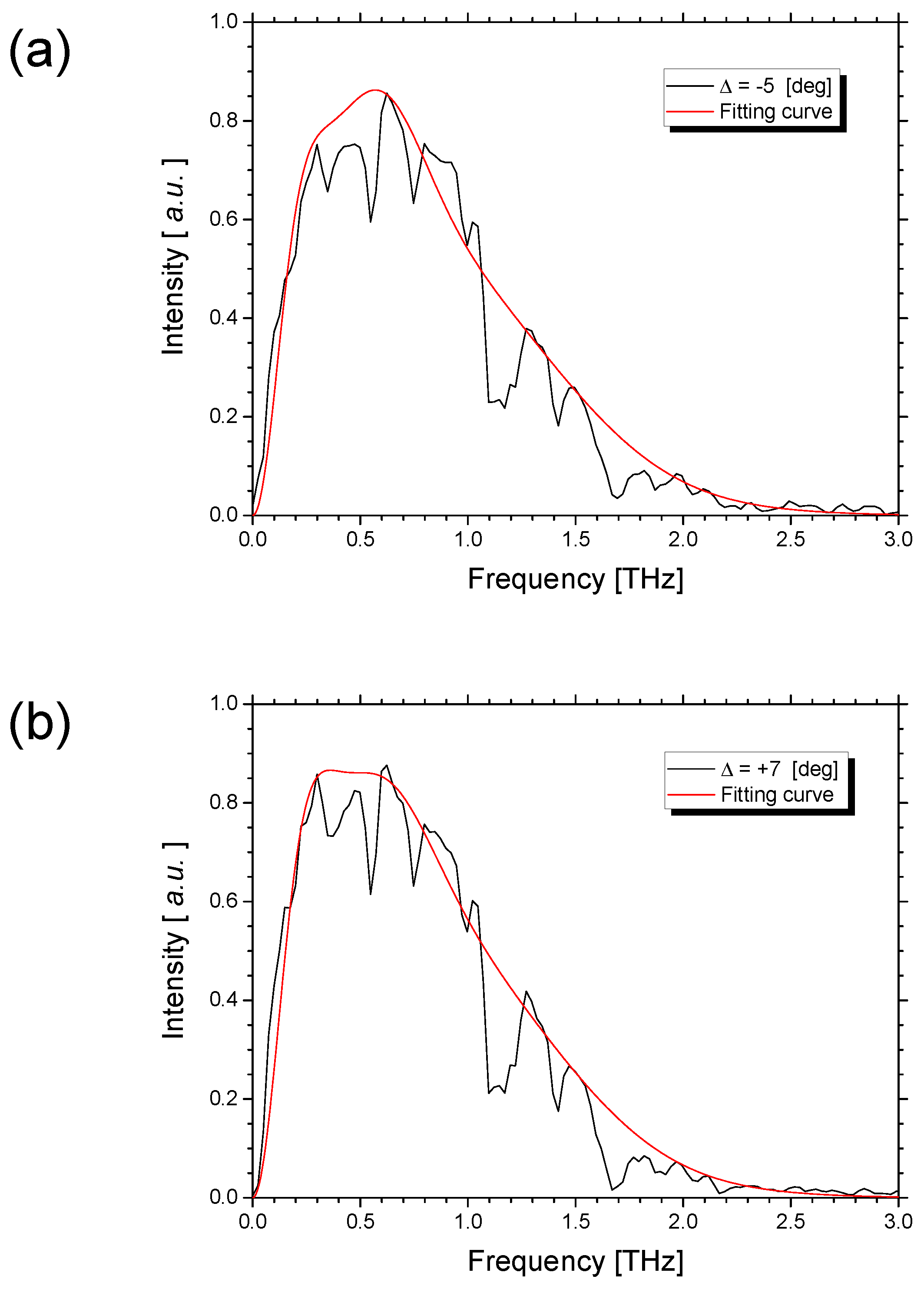
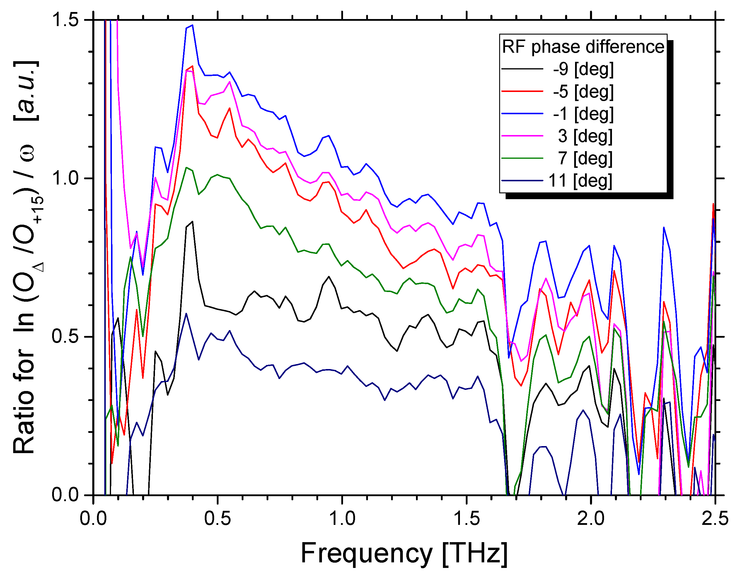
2.4. Change in the Form Factor for RF Phase

When the RF phase difference was +15 degrees, the electron bunch shape could be approximated by a Gaussian distribution. Therefore, to investigate the dependence of the electron bunch shape on the RF phase difference, a ratio of the spectrum at the phase difference ∆ to the spectrum at the phase difference +15 degrees, O_∆/O₊₁₅, was calculated. Figure 4 shows a graph obtained by dividing the logarithm of this ratio by the angular frequency. It was found that the function ln(O_∆/O₊₁₅)/ω could be linearly approximated in a frequency region ranging from 0.4 to 1.6 THz where the CER intensity was sufficiently high and the diffraction loss was negligible. As the ratio O_∆/O₊₁₅ was equal to the ratio of the form factor, this function suggested that the form factor at the RF phase difference ∆, f_∆(ω), could be expressed with coefficients α_∆ and β_∆ as the following equation:

$$f_{\mathsf{\Delta }}\left(\omega \right)=C_q{f}_{+15}\left(\omega \right)\exp \left({\alpha }_{\mathsf{\Delta }}{\omega }^2+{\beta }_{\mathsf{\Delta }}\omega \right)$$

(5)

where f₊₁₅(ω) is the form factor at ∆ = +15° and can be approximated by Equation (4) in the frequency region higher than 0.4 THz. C_q is a coefficient that depends on the ratio of the electron number in the bunch that contributes to the form factor in the frequency region. The form factor was given by using Equation (4) for Equation (5) with three coefficients (a_∆, b_∆, and c_∆) as the following equation:

$$f_{\mathsf{\Delta }}\left(\omega \right)=\exp \left(a_{\mathsf{\Delta }}{\omega }^2+b_{\mathsf{\Delta }}\omega +c_{\mathsf{\Delta }}\right)$$

(6)

As the form factor had to be under 1 [24], a_∆ was negative.

Table 1. Coefficients calculated by the least squares method for the measured spectra shown in Figure 3.

RF Phase Difference (Degree)	a∆/(2π)2	b∆/2π	Coefficient of Determination
−9	−1.09 × 10−24 ± 2.08 × 10−26	8.50 × 10−13 ± 2.86 × 10−14	0.9934
−5	−1.20 × 10−24 ± 1.80 × 10−26	1.31 × 10−12 ± 2.52 × 10−14	0.9944
−1	−1.24 × 10−24 ± 1.81 × 10−26	1.51 × 10−12 ± 2.58 × 10−14	0.9938
3	−1.30 × 10−24 ± 1.93 × 10−26	1.49 × 10−12 ± 2.64 × 10−14	0.9942
7	−1.18 × 10−24 ± 1.98 × 10−26	1.12 × 10−12 ± 2.72 × 10−14	0.9939
11	−1.05 × 10−24 ± 1.97 × 10−26	6.29 × 10−13 ± 2.64 × 10−14	0.9948

shows the coefficients a_∆/(2π)² and b_∆/2π calculated, which were calculated using the least squares method for the measured spectra shown in Figure 3. It was found that the coefficient of determination was close to 1 in the fitting calculation for any spectrum and the form factor could be expressed with Equation (6). The frequency at which the measured CER spectrum was maximized was highest on-crest operation of the RF field. The frequency, f_M, at which the calculated form factor was maximized was given by −b_∆π/a_∆ from Equation (6), and it was also highest on-crest operation as shown in Figure 5. Furthermore, it was clarified that f_M was given by the quadratic equation of the RF phase difference near the crest of the RF field.

3. Evaluation of the Electron Bunch Shape by Using Electron Distribution Models

3.1. Pseudo-Voigt Distribution

Although the form factor given by Equation (6) was evaluated from the measured CER spectrum in a limited frequency region, it contained information on the rough longitudinal shape of the electron bunch. Therefore, by simplifying the longitudinal structure of the electron bunch, we investigated the outline of the electron bunch. When the electron bunch shape is symmetric, S (z) is given with the square root of the form factor by the following equation [25]:

$$S\left(z\right)=\frac{1}{\pi c}{\displaystyle {\int }_0^{\infty }\sqrt{f\left(\omega \right)}}\cos \left(\frac{\omega }{c}z\right)d\omega$$

(7)

Here, the right side of Equation (7) is the inverse Fourier transform for the square root of the form factor. That is, when a Fourier transform for a function g is expressed as F[g], the following equation holds:

$$S\left(z\right)=F^{-1}\left[\sqrt{f\left(\omega \right)}\right]$$

(8)

Using the convolution theorem for the Fourier transform

$$F^{-1}\left[g_1\cdot g_2\right]=\frac{1}{2\pi }{F}^{-1}\left[g_1\right]*F^{-1}\left[g_2\right]$$

(9)

$$g_1\left(x\right)*g_2\left(x\right)\equiv {\displaystyle \int g_1}\left(x-y\right)g_2\left(y\right)dy$$

(10)

S (z) can be expressed with Equation (6) as the following equation [26]:

$$S\left(z\right)=\frac{e^{\frac{1}{2}{c}_{\mathsf{\Delta }}}}{4{\pi }^2}{F}^{-1}\left[e^{\frac{1}{2}{a}_{\mathsf{\Delta }}{\omega }^2}\right]*F^{-1}\left[e^{\frac{1}{2}{b}_{\mathsf{\Delta }}\left|\omega \right|}\right]$$

(11)

If both a_Δ and b_Δ are negative, the righthand side in Equation (11) is a convolution of the Gaussian and Lorentz function. Therefore, under this assumption, S (z) can be described with a Voigt function V(z;σ,γ_L) as the following equations:

$$S\left(z\right)=\frac{e^{\frac{1}{2}{c}_{\mathsf{\Delta }}}}{4{\pi }^2}V\left(z;\sigma ,{\gamma }_L\right)$$

(12)

$$\sigma =c\sqrt{-a_{\mathsf{\Delta }}}$$

(13)

$${\gamma }_L=-\frac{1}{2}{b}_{\mathsf{\Delta }}c$$

(14)

As it is difficult for the Voigt function to capture the outline of the distribution, a pseudo-Voigt function consisted of elementary functions is often used instead of the Voigt function in spectroscopy [27,28]. When the full width at half maximum of the Voigt function is defined as w_v, S (z) can be approximated as the following equation [29,30]:

$$\begin{array}{ll}S\left(z\right)& =\frac{e^{\frac{1}{2}{c}_{\mathsf{\Delta }}}}{4{\pi }^2}{V}_{pV}\left(z;w_V,\eta \right)\\ & =\frac{e^{\frac{1}{2}{c}_{\mathsf{\Delta }}}}{4{\pi }^2}\left[\left(1-\eta \right)\frac{2}{w_V}\sqrt{\frac{\ln 2}{\pi }}{e}^{-\frac{4\ln 2}{w_V^2}{z}^2}+\eta \frac{2w_V}{\pi \left(w_V^2+4z^2\right)}\right]\end{array}$$

(15)

where η represents the ratio of the Lorentz component, and the pseudo-Voigt function is physically meaningful in the case of 0 ≤ η ≤ 1.

Nevertheless, herein, we consider the case in which η is negative. As the asymptotic behavior of the pseudo-Voigt function becomes negative in the case of η < 0, it is not usually treated as a distribution function. However, it is possible to avoid the negative distribution function by making a section in which the electrons are distributed finitely and by adding a positive constant term. When the behavior of the form factor in the low frequency region is ignored, it is possible to add a Gaussian distribution term with a large standard deviation instead of the positive constant term. The physical meaning of the additional term is a background composed of low density electrons around the main components of the electron bunch, which has been actually observed in linear accelerators [31]. Figure 6 shows an electron distribution given by a pseudo-Voigt function with a negative η and its form factor. To avoid the negative electron distribution, a Gaussian distribution with a standard deviation of 5.0 mm, which is 100 times the standard deviation of the pseudo-Voigt function, is added as an additional term. As shown in Figure 6, there is a local maximum of the form factor at a frequency that is away from zero. The coefficient b_∆ in Equation (6) was negative in the observed CER spectrum, therefore, the function of the electron distribution in the bunch could not be expressed as in Equation (11). However, by using a pseudo-Voigt function with a negative η, it is possible to reproduce a structure similar to the observed CER spectrum.

Although there are numerous spectra described by the pseudo-Voigt function in the frequency domain, few physical quantities distributed by the pseudo-Voigt function in the time domain have been reported. The electrons in the bunch rotate 90° counterclockwise in a phase space by passing through the 180° arc section [32], which consists of two axes, the position in the traveling direction and the energy. The fact that the electron bunch had a distribution described by the pseudo-Voigt function suggests that the electron energy after passing through the acceleration tube had the pseudo-Voigt function distribution.

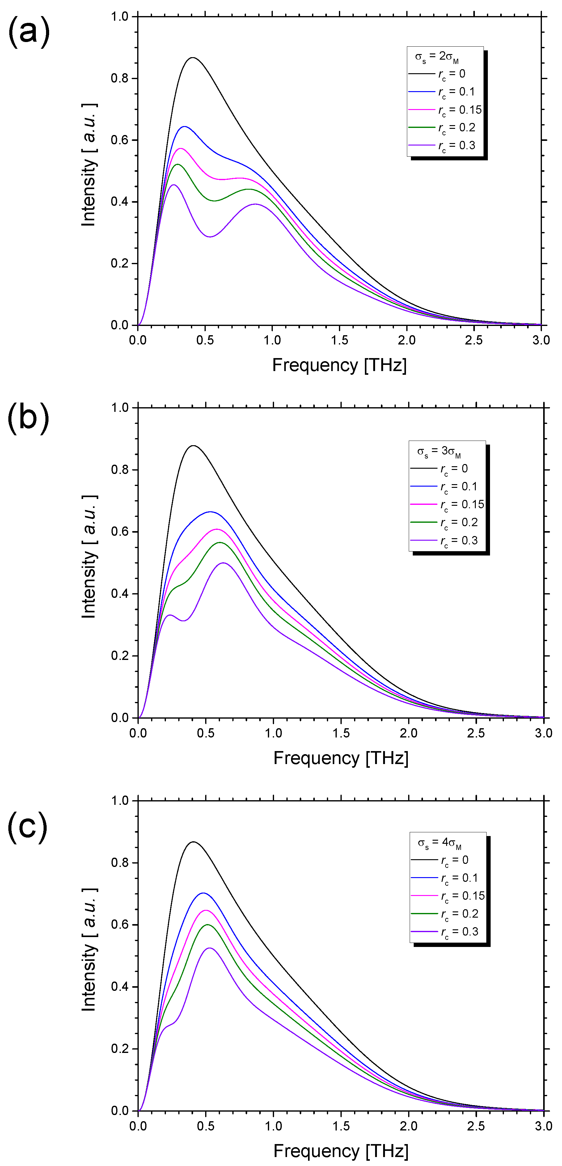
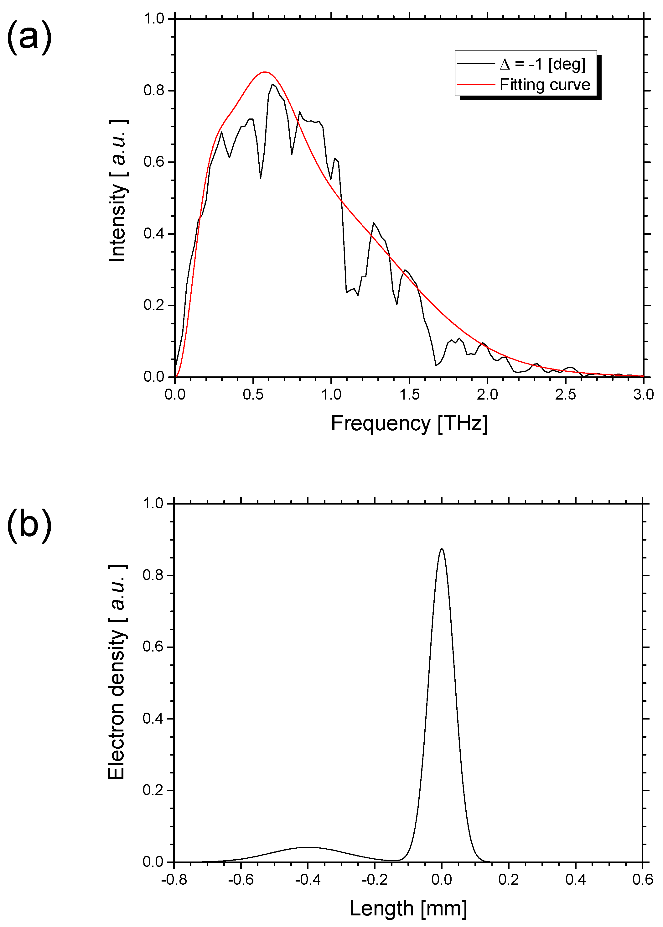
3.2. Satellite Pulse Model for Electron Bunch

The electron distribution expressed by a pseudo-Voigt function with a negative η could describe the observed CER spectrum by adding a term that made the electron distribution positive. However, the proportion of the electrons that form the main peak of the electron bunch is reduced by the additional component with a larger variance, and the CER power is significantly reduced although the total charge in the electron bunch remains unchanged. The CER energy on-crest operation of the RF field was 0.12 mJ per macropulse, which was approximately 0.6 times the energy calculated with the CER theory. Most of the electrons contributed to the formation of the main pulse in the electron bunch, and a more realistic model of the electron distribution would be needed to describe the measured spectrum. As shown in Figure 6, a dip appears beside the main peak in the pseudo-Voigt function with a negative η. As the absolute value of η is larger, the dip is deeper and the frequency at which the form factor is maximized is higher. It is noted that the dip of the electron distribution in the bunch concerns the local maximum appearing in the CER spectrum. In fact, electron distributions in the bunch with a dip structure have been reported at some linac facilities [33,34,35].

Therefore, as a simple model that can create a dip in a bunch shape, we consider a satellite pulse model in which a small pulse exists around a main pulse with most of the electrons. For simplicity, the electron distributions of the two pulses are assumed to be Gaussian. Furthermore, it is assumed that the RMS bunch length of the satellite pulse is larger than that of the main pulse and the charge of the satellite pulse is 0.3 times or less than that of the main pulse. Based on these assumptions, the contribution of the satellite pulse to the CER power is less than 1/10 that of the main pulse, and only the bunch shape of the main pulse contributes to the high frequency components of the CER spectrum. Figure 7 shows the RMS bunch length σ_M of the main pulse evaluated by fitting the measured CER spectrum to Equation (4) in the frequency region of 1–2 THz. The RMS bunch length evaluated from the CER spectrum behaved non-linearly with respect to the RF phase difference and became minimal near the crest. As the electrons in the bunch rotated 90° in the phase space by passing through the 180° arc, the energy distribution of the electron bunch after passing through the accelerator tube was considered to have the same dependence on the RF phase difference as the electron distribution in the undulator straight section. It was confirmed that the relationship between the RMS electron bunch length and the RF phase difference evaluated with the CER spectra was similar to the relationship between the RMS energy spread and the RF phase difference, which was reported at a linear accelerator facility [36].

Next, we consider the satellite pulse in the electron bunch. The satellite pulse has three independent parameters: the RMS bunch length σ_S, the distance from the main pulse ∆_p, and the ratio of the charge to the main pulse r_c. A deep dip is required to increase the frequency of the local maximum in the CER spectrum. When a constant d₁ is expressed with ∆_p as

$${\mathsf{\Delta }}_p=d_1\left({\sigma }_S+{\sigma }_M\right)$$

(16)

the intensity of each pulse at the intersection of both the pulses is 5% of its peak value in the case of d₁ = 2.5, and a dip becomes sufficiently deep. Figure 8 shows the CER spectra calculated in the cases of σ_S = 2σ_M, 3σ_M, and 4σ_M. The transmittance and diffraction loss of the optical transport system shown in Equation (1) are taken into consideration in these CER spectra calculated for some r_c. As shown in Figure 8, it can be noted that the frequency of the maximum of the CER spectrum at d₁ = 3 shifts to the high frequency side and exceeds 0.6 THz as r_c increases. Moreover, the modulation in the CER spectrum grows as r_c increases. The observed CER spectrum had a maximum on-crest operation at a frequency of approximately 0.6 THz, but there was no significant modulation in the CER spectrum. It is estimated that r_c was 0.15 from the CER spectrum calculated by changing r_c. Therefore, the CER spectra are calculated by changing ∆_p in conditions of σ_S = 3σ_M and r_c = 0.15 as shown in Figure 9. It is noted that the coordinates of the maximum move counterclockwise in the graph as the distance between the main and satellite pulses increases from zero. The frequency of the maximum is maximized when the distance is 10.5σ_M. Therefore, we compare the calculated CER spectrum in the case of (σ_S, ∆_p, r_c) = (3σ_M, 10.5σ_M, 0.15) to the measured CER spectrum near the crest, O₋₁, as shown in Figure 10a. The electron bunch shape in this condition is shown in Figure 10b. The coefficient of determination of the calculated CER spectrum for the set of frequencies used in Section 2.3 is as high as 0.983, it was found that the satellite pulse model can effectively reproduce the CER spectrum near the crest.

As described in Section 2.2, the electron distribution in the bunch can be approximated by the Gaussian at the RF phase difference of +15 degrees. Figure 9 shows that the distance between the main and satellite pulses is almost zero at this RF phase difference. As proved in Appendix A, when the satellite pulse has a lower energy than the main pulse, the distance between the main and satellite pulses changes from the initial state on-crest operation by an amount proportional to the square of the RF phase difference. In fact, the frequency of the maximum of the form factor fitted by Equation (6) was given as a quadratic function of the RF phase difference. Therefore, the distance between the main and satellite pulses can be given by

$${\mathsf{\Delta }}_p=-d_2{\mathsf{\Delta }}^2+10.5{\sigma }_M$$

(17)

where a constant d₂ is determined so that Δ_p becomes zero at ∆ = +15°. Figure 11 shows spectra fitted for ∆ = −5° and +7° with ∆_p calculated by Equation (16) and σ_M shown in Figure 7. The ratio r_c is assumed to be 0.15 in these fittings. The coefficients of determination for these fitting curves are 0.988 for ∆ = −5° and 0.991 ∆ = +7°, respectively. Although the satellite pulse model does not describe the complex structure of the measured CER spectrum, it can explain that there is a frequency fluctuating local maximum due to the RF phase difference in the CER spectrum. It was confirmed that this simplified model is a good representation of the outline of the electron bunch shape.

4. Discussion

We observed the CER spectra generated by electron beams passing through the downstream bending magnet of the undulator straight section at KU-FEL. It was observed that the CER spectrum had a local maximum on-crest operation of the RF field at the electron energy of 40 MeV. The frequency of the maximum depended on the RF phase difference between the electron gun and the accelerating tube. The frequency was maximized near the crest and decreased in proportion to the square of the RF phase difference from the crest. The form factor evaluated from the measured CER spectrum was proportional to a function whose exponent was given by the quadratic equation of the frequency. These experimental results suggest that the longitudinal electron distribution in the bunch can be approximated by the pseudo-Voigt function in the real space. Although there are many phenomena in which the Voigt distribution appears in the frequency space as in the Raman spectroscopy, it is rare that a distribution in the real space is described by the pseudo-Voigt function.

However, a negative electron distribution appears in the pseudo-Voigt function with a negative ratio η. Therefore, we proposed a satellite pulse model consisting of two pulses with a large and small amount of charge as a practical model for the electron distribution. This model shows that the frequency at which the CER spectrum is maximized depends on the interval between the two pulses. It is preferable to evaluate the electron bunch shape using the Kramers–Kronig relation for more complex spectral structures [25,33]. However, the accuracy of the measurement for the low frequency components of the CER spectrum is low due to the cutoff of the optical transport system and the sensitivity of the detector, and it is difficult to accurately reproduce the electron bunch shape. The satellite pulse model is effective in describing the outline of the electron distribution in the bunch despite its simplicity.

As described above, it is possible to investigate the longitudinal distribution in the electron bunch by observing the CER spectrum. We improved the flat mirror so that the CER during FEL oscillations can be observed without damaging the FEL oscillation, and we observed that the FEL oscillations cause changes in the CER spectrum. Furthermore, in order to remove the influence of absorption by water vapor, we will consider placing the CER observation system under dry air. The measurements of the CER spectrum during FEL oscillations will elucidate the effect of the FEL interactions on the longitudinal electron bunch shape. The CER is the best tool to understand how the electron bunch is influenced by the FEL interaction.

References

1. Kovalev, S.; Wang, Z.; Deinert, J.-C.; Awari, N.; Chen, M.; Green, B.; Germanskiy, S.; Oliveira, T.; Lee, J.S.; Deac, A.; et al. Selective THz control of magnetic order: New opportunities from superradiant undulator sources. J. Phys. D Appl. Phys. 2018, 51, 114007. [Google Scholar] [CrossRef] [Green Version]
2. Sei, N.; Takahashi, T. Terahertz-wave spectrophotometry by Compton backscattering of coherent transition radiation. Appl. Phys. Express 2010, 3, 052401. [Google Scholar] [CrossRef]
3. Sei, N.; Ogawa, H.; Hayakawa, K.; Tanaka, T.; Hayakawa, Y.; Nakao, K.; Sakai, T.; Nogami, K.; Inagaki, M. Complex light source composed from subterahertz-wave coherent synchrotron radiation and an infrared free-electron laser at the Laboratory for Electron Beam Research and Application. J. Opt. Soc. Am. B 2014, 31, 2150–2156. [Google Scholar] [CrossRef]
4. Tonouchi, M. Cutting-edge terahertz technology. Nat. Photonics 2007, 1, 97–105. [Google Scholar] [CrossRef]
5. Kung, P.; Lihn, H.; Wiedemann, H.; Bocek, D. Generation and Measurement of 50-fs (rms) Electron Pulses. Phys. Rev. Lett. 1994, 73, 967–970. [Google Scholar] [CrossRef] [Green Version]
6. Lumpkin, A.H.; Sereno, N.S.; Rule, D.W. First measurements of subpicosecond electron beam structure by autocorrelation of coherent diffraction radiation. Nucl. Instrum. Methods Phys. Res. A 2001, 475, 470–475. [Google Scholar] [CrossRef] [Green Version]
7. Castellano, M.; Verzilov, V.A.; Catani, L.; Cianchi, A.; Orlandi, G.; Geitz, M. Measurements of coherent diffraction radiation and its application for bunch length diagnostics in particle accelerators. Phys. Rev. E 2001, 63, 056501. [Google Scholar] [CrossRef]
8. Ha, G.; Power, J.G.; Shao, J.; Conde, M.; Jing, C. Coherent synchrotron radiation free longitudinal bunch shaping using transverse deflecting cavities. Phys. Rev. Accel. Beams 2020, 23, 072803. [Google Scholar] [CrossRef]
9. Andonian, G.; Dunning, M.; Hemsing, E.; Rosenzweig, J.B.; Cook, A.; Murokh, A.; Vicario, C.; Kusche, K.; Yakimenko, V.; Alesini, D.; et al. Observation of Coherent Edge Radiation Emitted by a 100 Femtosecond Compressed Electron Beam. Int. J. Mod. Phys. A 2007, 22, 4101–4114. [Google Scholar] [CrossRef]
10. Grimm, O. Synchrotron radiation for beam diagnostics: Numerical calculations of the single electron spectrum. TESLA-FEL Rep. 2008, 5, 2008. [Google Scholar]
11. Sei, N.; Sakai, T.; Hayakawa, Y.; Sumitomo, Y.; Nogami, K.; Tanaka, T.; Hayakawa, K. Observation of terahertz coherent edge radiation amplified by infrared free-electron laser oscillations. Sci. Rep. 2021, 11, 3433. [Google Scholar] [CrossRef]
12. Sei, N.; Zen, H.; Ohgaki, H. Measurement of bunch length evolution in electron beam macropulse of S-band linac using coherent edge radiation. Phys. Lett. A 2019, 383, 389–395. [Google Scholar] [CrossRef]
13. Ohgaki, H.; Kii, T.; Masuda, K.; Zen, H.; Sasaki, S.; Shiiyama, T.; Kinjo, R.; Yoshikawa, K.; Yamazaki, T. Lasing at 12 µm Mid-Infrared Free-Electron Laser in Kyoto University. Jpn. J. Appl. Phys. 2008, 47, 8091–8094. [Google Scholar] [CrossRef]
14. Zen, H.; Ohgaki, H. Study of the origin of the complex beam profile of a hole-coupled free electron laser oscillator. J. Opt. Soc. Am. A 2021, 38, 1656–1661. [Google Scholar] [CrossRef]
15. Sei, N.; Zen, H.; Ohgaki, H. Development of intense terahertz coherent synchrotron radiation at KU-FEL. Nucl. Instrum. Methods Phys. Res. A 2016, 832, 208–213. [Google Scholar] [CrossRef]
16. Nagai, R.; Kobayashi, H.; Sasaki, S.; Sawamura, M.; Sugimoto, M.; Kato, R.; Kikuzawa, N.; Ohkubo, M.; Minehara, E.; Ikehata, T.; et al. Performance of the undulator for JAERI FEL project. Nucl. Instrum. Meth. A 1995, 358, 403–406. [Google Scholar] [CrossRef]
17. Available online: http://hitran.iao.ru/home (accessed on 29 October 2021).
18. Evtushenko, P.; Coleman, J.; Jordan, K.; Klopf, J.M.; Neil, G.; Williams, G.P. Bunch Length Measurements at JLab FEL. In Proceedings of the 28th Free Electron Laser Conference, Berlin, Germany, 27 August 2006; pp. 736–739. [Google Scholar]
19. Grischkowsky, D.; Keiding, S.; Exter, M.; Fattinger, C.J. Far-infrared time-domain spectroscopy with terahertz beams of dielectrics and semiconductors. Opt. Soc. Am. B 1990, 7, 2006–2015. [Google Scholar] [CrossRef]
20. Blea, J.M.; Parks, W.F.; Ade, P.A.R.; Bell, R.J. Optical Properties of Black Polyethylene from 3 to 4000 cm−1. J. Opt. Soc. Am. 1970, 60, 603–606. [Google Scholar] [CrossRef]
21. Ganichev, S.D.; Prettl, W. Intense Terahertz Excitation of Semiconductors; OUP Oxford: Oxford, UK, 2006; p. 432. [Google Scholar]
22. Nakazato, T.; Oyamada, M.; Niimura, N.; Urasawa, S.; Konno, O.; Kagaya, A.; Ikezawa, M.; Kato, R.; Kamiyama, T.; Torizuka, Y.; et al. Observation of coherent synchrotron radiation. Phys. Rev. Lett. 1989, 63, 1245–1248. [Google Scholar] [CrossRef]
23. Shibata, Y.; Takahashi, T.; Kanai, T.; Ishi, K.; Ikezawa, M.; Ohkuma, J.; Okuda, S.; Okada, T. Diagnostics of an electron beam of a linear accelerator using coherent transition radiation. Phys. Rev. E 1994, 50, 1479–1484. [Google Scholar] [CrossRef]
24. Carr, G.L.; Martin, M.C.; McKinney, W.R.; Jordan, K.; Neil, G.R.; Williams, G.P. High-power terahertz radiation from relativistic electrons. Nature 2001, 420, 153–156. [Google Scholar] [CrossRef] [PubMed]
25. Grimm, O.; Schmuser, P. Principles of Longitudinal Beam Diagnostics with Coherent Radiation. TESLA-FEL Rep. 2006, 1040. [Google Scholar]
26. Mitra, G.B. Theoretical Model of Diffraction Line Profiles as Combinations of Gaussian and Cauchy Distributions. J. Cryst. Process Technol. 2014, 4, 145–155. [Google Scholar] [CrossRef] [Green Version]
27. Jacobs, P.; Houben, A.; Schweika, W.; Tchougreeff, A.L.; Dronskowski, R. Instrumental resolution as a function of scattering angle and wavelength as exemplified for the POWGEN instrument. J. Appl. Cryst. 2017, 50, 866–875. [Google Scholar] [CrossRef] [Green Version]
28. Leménager, G.; Tusseau-Nenez, D.; Thiriet, M.; Coulon, P.E.; Lahlil, K.; Larquet, E.; Gacoin, T. NaYF4 Microstructure, beyond Their Well-Shaped Morphology. Nanomaterials 2019, 9, 1560. [Google Scholar] [CrossRef] [PubMed] [Green Version]
29. Wertheim, G.K.; Butler, M.A.; West, K.W.; Buchanan, D.N.E. Determination of the Gaussian and Lorentzian content of experimental line shapes. Rev. Sci. Instrum. 1974, 45, 1369–1371. [Google Scholar] [CrossRef]
30. David, W.I.F. Powder diffraction peak shapes. Parameterization of the pseudo-Voigt as a Voigt function. J. Appl. Crystallogr. 1986, 19, 63–64. [Google Scholar] [CrossRef]
31. Hüning, M.; Bolzmann, A.; Schlarb, H.; Frisch, J.; McCormick, D.; Ross, M.; Smith, T.; Rossbach, J. Observation of Femtosecond Bunch Length Using a Transverse Deflecting Structure. In Proceedings of the 27th Free Electron Laser Conference, Stanford, CA, USA, 21–26 August 2005; pp. 538–540. [Google Scholar]
32. Zen, H.; Kii, T.; Masuda, K.; Ohgaki, H.; Sasaki, S.; Shiiyama, T. Numerical study on the optimum cavity voltage of RF gun and bunch compression experiment in KU-FEL. In Proceedings of the 29th Free Electron Laser Conference, Novosibirsk, Russia, 26–31 August 2007; pp. 402–405. [Google Scholar]
33. Behrens, C.; Gerasimova, N.; Gerth, C.; Schmidt, B.; Schneidmiller, E.A.; Serkez, S.; Wesch, S.; Yurkov, M.V. Publisher’s Note: Constraints on photon pulse duration from longitudinal electron beam diagnostics at a soft X-ray free-electron laser. Phys. Rev. ST Accel. Beams 2012, 15, 069902. [Google Scholar] [CrossRef]
34. Wu, Z.; Fisher, A.S.; Goodfellow, J.; Fuchs, M.; Daranciang, D.; Hogan, M.; Loos, H.; Lindenberg, A. Intense terahertz pulses from SLAC electron beams using coherent transition radiation. Rev. Sci. Instrum. 2013, 84, 022701. [Google Scholar] [CrossRef]
35. Curcio, A.; Bergamaschi, M.; Corsini, R.; Farabolini, W.; Gamba, D.; Garolfi, L.; Senes, E.; Kieffer, R.; Lefevre, T.; Mazzoni, S.; et al. Noninvasive bunch length measurements exploiting Cherenkov diffraction radiation. Phys. Rev. Accel. Beams 2020, 23, 022802. [Google Scholar] [CrossRef] [Green Version]
36. Yang, J.; Kuroda, Y.; Kan, K.; Kondoh, T.; Kozawa, T.; Yoshida, Y.; Tagawa, S. Generation of Double-Decker Femtosecond Electron Beams in a Photoinjector. In Proceedings of the 2005 Particle Accelerator Conference, Knoxville, TN, USA, 16–20 May 2005; pp. 1604–1606. [Google Scholar]
37. Serafini, L.; Ferrario, M. Velocity bunching in photo-injectors. AIP Conf. Proc. 2001, 581, 87–106. [Google Scholar]
38. Piot, P.; Carr, L.; Graves, W.S.; Loos, H. Subpicosecond compression by velocity bunching in a photoinjector. Phys. Rev. ST Accel. Beams 2003, 6, 033503. [Google Scholar] [CrossRef] [Green Version]
Figure 1. Schematic outline of KU-FEL and observation system for the CER beam.
Applsci 12 00626 g001
Figure 2. Relationship between the RF phase difference and the measured FEL macropulse.
Applsci 12 00626 g002
Figure 3. (a) Relationship between the RF phase difference and measured CER spectrum. (b) Fitting curve (red dotted curve) applying the least squares approximation to the measured CER spectrum (black solid curve) for ∆ = +15°.
Applsci 12 00626 g003
Figure 4. Relationship between the logarithm of ratio O/O+15 divided by angular frequency and the frequency.
Applsci 12 00626 g004
Figure 5. Dependence of fM on RF phase difference ∆. The fitting curve (broken red line) is given by fM = −2.66 × 1092 + 6.06 × 10¹¹.
Applsci 12 00626 g005
Figure 6. (a) Electron distribution based on a pseudo-Voigt function with wV = 90 μm and η = −0.8. The area and standard deviation of the additional Gaussian distribution are 5.4 and 100 times the Gaussian distributions that constitute the pseud-Voigt function, respectively. (b) Form factor spectrum calculated for the electron distribution in (a).
Applsci 12 00626 g006
Figure 7. Evaluated RMS bunch length of the main pulse for the measured CER spectrum at ∆ = +15° in the satellite pulse model.
Applsci 12 00626 g007
Figure 8. Calculated CER spectra for several rc in the cases of σS = (a) 2σM, (b) 3σM, and (c) 4σM. Here, σM is 38.0 μm and d1 is 2.5.
Applsci 12 00626 g008
Figure 9. Calculated CER spectra for several ∆p with σS = 3σM and rc = 0.15.
Applsci 12 00626 g009
Figure 10. (a) Calculated CER spectrum in the satellite pulse model (red curve) and the measured CER spectrum for ∆ = −1° (black curve). The parameters σS, ∆p, rc are 3σM, 10.5σM, and 0.15, respectively. (b) Electron distribution at the aforementioned parameters in the satellite pulse model.
Applsci 12 00626 g010
Figure 11. Fitting curves for the CER spectra at (a) ∆ = −5° and (b) ∆ = +7° (red curves). The measured spectra are indicated by black curves in the figures.
Applsci 12 00626 g011