Effects of Evaporative Emissions Control Measurements on Ozone Concentrations in Brazil

Abstract

In this work, the possible benefits obtained due to the implementation of evaporative emissions control measures, originating from vehicle fueling processes, on ozone concentrations are verified. The measures studied are: (1) control at the moment when the tank trucks supply the fuel to the gas stations (Stage 1); (2) control at the moment when the vehicles are refueled at the gas stations, through a device installed in the pumps (Stage 2); (3) same as the previous control, but through a device installed in the vehicles (ORVR). The effects of these procedures were analyzed using numerical modeling with the VEIN and WRF/Chem models for a base case in 2018 and different emission scenarios, both in 2018 and 2031. The results obtained for 2018 show that the implementation of Stages 1 and 2 would reduce HCNM emissions by 47.96%, with a consequent reduction of 19.9% in the average concentrations of tropospheric ozone. For 2031, the greatest reductions in ozone concentrations were obtained with the scenario without ORVR, and with Stage 1 and Stage 2 (64.65% reduction in HCNM emissions and 31.93% in ozone), followed by the scenario with ORVR and with Stage 1 and Stage 2 (64.39% reduction in HCNM emissions and 32.98% in ozone concentrations).

1. Introduction

Brazil has a vehicular fleet of more than 100 million registered vehicles, according to the National Department of Traffic [1]. This vehicular fleet impacts air quality with deleterious effects on the population’s health and on ecosystems [2]. The vehicle fleet is responsible for most of the primary emissions of carbon monoxide (CO), nitrogen oxides (NOx), and non-methane hydrocarbons (NMHC) [3]. NOx and NMHC lead to the formation of tropospheric ozone (O₃). Tropospheric ozone is generated, primarily, by the interaction of volatile organic compounds, nitrogen oxides, and solar radiation with health and vegetation impacts [4,5,6,7]. The Metropolitan Area of São Paulo (MASP), with a population of 22 million people, presents high concentrations of this gas, exceeding the recommended values to guarantee air quality [8,9,10,11]. Evaporative emissions are an important source of NMHC [12,13]. Decreasing the emissions of precursor gases (NMHC and NOx) according to atmospheric reactivity is one of the possible ways to decrease the concentrations of tropospheric ozone.

Since 1986, specific Brazilian legislation has been applied in order to reduce vehicular emissions [14], and after that many works have analyzed the benefits of the Air Pollution Control Program for Motor Vehicles (PROCONVE) and have shown that most of the primary pollutants had their concentrations considerably reduced in the atmosphere [15,16]. However, the same works have also shown that secondary pollutants, such as ozone, do not follow the same pattern, even with an increase in its concentration over the years. The most recent legislation in Brazil with the goal of reducing evaporative emissions, partially responsible for ozone formation, was established in 2018, with new PROCONVE phases defining new emission limits for vehicles from 2022, with staggered deployment over the following years [17]. The new phases of PROCONVE impose the use of the Onboard Refueling Vapor Recovery system (ORVR) on all new vehicles until 2025. However, other important sources of evaporative emissions will still be without any control at least until 2031, when an Employment Law will require the installation of emission control systems in the gas station pumps, controlling the emissions at the moment when the vehicles are refueled at the gas stations, which is being called Stage 2. Besides this, the evaporative emissions at the moment when the tank trucks supply the fuel to the gas stations are not part of any emission control plan in Brazil, which will constitute great harm for the population, since those emissions will still be important for secondary pollutant formation, possibly causing damage to human health.

In order to analyze the effectiveness of evaporative control measures on air quality, this work presents the results of simulations of the ozone concentration considering the impacts of the control of the evaporative emissions resulting at the moment when the tank trucks fill the gas stations (Stage 1) and when the vehicles are filled at the gas stations (Stage 2 and ORVR). The results correspond to the analyses of two periods: (i) reference, with atmospheric and emission conditions for the year 2018, and (ii) considering future emissions in 2031, but with the same atmospheric conditions of the year 2018.

2. Materials and Methods

The emissions related to road transport were estimated for Brazil and then, for MASP area, we used spatially allocated emissions based on the outputs of travel demand models for light vehicles and trucks, provided by Traffic Engineer Company CET (http://cetsp.com.br/, accessed on 21 December 2021) and Urban Buses (UB) from Sao Paulo Transit System SPTRANS (http://www.sptrans.com.br/, accessed on 21 December 2021) using the Vehicle Emissions Model (VEIN [18]), a package written in the free access R language (available at https://CRAN.R-project.org/package=vein, accessed on 21 December 2021), which allows the inclusion of different features of the fleet, with the possibility of considering traffic flow and speed by using GPS data [19,20]. The vehicular composition was obtained from the official inventory of the CETESB (São Paulo State’s Environmental Agency) adjusted by fuel consumption [20]. The emission factors come from an association among emission inventories provided by CETESB, field experiments made by the air quality group from IAG-USP, and surface measurements in different locations in the MASP. In 2018, the fleet already had PROCONVE phase L6 vehicles, which are equivalent to Euro 5 (https://www.transportpolicy.net/standard/brazil-light-duty-emissions/, accessed on 21 December 2021). For this phase, the vehicle emissions inventory made available by CETESB estimates that the evaporation occurs in accordance with the ABNT NBR 11481 standard, based on the measurements performed on “Sealed Housing for Evaporative Determination” (SHED) equipment, a sealed chamber in which the fuel vapor is measured at the end of the two-phase test: the “diurnal” phase, as a result of exposure to the sun with the cold vehicle, and the “hot” phase, due to the engine heating after use. For the measurement of evaporative emissions with “SHED 1 + 1,” in the “diurnal” phase, the vehicle is placed in the SHED chamber and the fuel tank is heated to a temperature of 16 °C to 28 °C for 1 h, during which the vapor measurements are made. With the vehicle’s engine warmed up after running a dynamometer urban driving cycle, according to NBR 6601, 2 min after the engine is switched off, the vehicle is placed back on the SHED, for the measurement of the “hot” phase, where it remains for another hour, new measurements of the emitted vapors being made. In the process, evaporative emissions during vehicle operation, which are called “running losses,” are also considered [21]. After the publication of the decrees that regulate the new phases of PROCONVE [17], including phase L7, the protocol for the measurements of the “diurnal” and “hot” phases were changed, with an extension of the period used. For the PROCONVE L7 phase, the maximum emission limit for fuel evaporated by gasoline, ethanol, or flex vehicles is 0.5 g per day of testing, which is carried out over a continuous period of 48 h. These emissions were considered by VEIN and used during the simulations made in this work for both years, 2018 and 2031. The refueling emissions are calculated from fuel consumption, 1.14 g/L for gasoline (gasoline with 27% ethanol) and 0.37 g/L for ethanol [21]. The evaporative emission factors diurnal (g/day), running losses (g/test), and hot-soak (g/test) come from the official inventory published by CETESB. These emission factors, based on a legislative test, are used in the absence of real-world measurement of evaporative emission factors. The emissions factors with units of g/test (assumed as g/trip) and g/day are converted to g/km assuming 4.6 trips per day and dividing the mileage by 365, respectively, as explained by Ibarra-Espinosa et al. [20]. Subsequently, air quality simulations were performed using the Weather Research and Forecast meteorological model (WRF) with its activated photochemical module (WRF-Chem [22]). The input data related to emissions for WRF-Chem were arranged in the NetCDF format and were generated using the EIXPORT model [23]. Subsequently, air quality simulations were performed using the Weather Research and Forecast meteorological model (WRF) with its activated photochemical module (WRF-Chem [22]). The input data related to emissions for WRF-Chem were arranged in the NetCDF format and were generated using the EIXPORT model [23].

Ten scenarios were considered. The first three consider the base year of 2018 and the other seven consider the growth of the fleet and the implementation or not of the new phases of PROCONVE and also the emission controls provided by Stage 1 and Stage 2 in the gas stations. The configuration of the scenarios was based on the works of Fung and Maxwell [24] and US-EPA [25] with an efficiency of 100% for Stage 1, 90% for Stage 2, and 100% with ORVR for refueling emissions. Additionally, it was considered that the combination of ORVR and Stage 2 would increase emissions by 5% and that ORVR also controls diurnal emissions. The exhaust emissions factors for 2031 are the ones for the year 2018, and the change in exhaust emissions is due to fleet turnover. With the goal of simulating the impact of different evaporative emission controls on air quality, we considered the following scenarios for the years 2018 and 2031:

• 2018 baseline
  S0 Scenario 0: Base L6 (Shed 1 + 1) without ORVR, without Stage 1, without Stage 2 (fleet 2018).
  S1 Scenario 1: Base L6 (Shed 1 + 1) without ORVR, with Stage 1, without Stage 2 (fleet 2018).
  S2 Scenario 2: Base L6 (Shed 1 + 1) without ORVR, with Stage 1, with Stage 2 (fleet 2018).
• 2031 without ORVR
  S3 Scenario 3: Base L7 (Shed 0.5 48 h) without ORVR, with Stage 1, without Stage 2 (fleet 2031).
  S5 Scenario 5: Base L7 (Shed 0.5 48 h) without ORVR, with Stage 1, with Stage 2 (fleet 2031).
  S7 Scenario 7: Base L7 (Shed 0.5 48 h) without ORVR, without Stage 1, With Stage 2 (fleet 2031).
• 2031 with ORVR
  S4 Scenario 4: Base L7 (Shed 0.5 48 h) with ORVR, without Stage 1, without Stage 2 (fleet 2031).
  S6 Scenario 6: Base L7 (Shed 0.5 48 h) with ORVR, with Stage 1, with Stage 2 (fleet 2031).
  S8 Scenario 8: Base L7 (Shed 0.5 48 h) with ORVR, without Stage 1, with Stage 2 (fleet 2031).
• 2031 without ORVR, without Stage 2, and without Stage 1 (future reference)
  S9 Scenario 9: Base L7 (Shed 0.5 48 h) without ORVR, without Stage 1, without Stage 2 (fleet 2031).

As mentioned before, numerical simulations were performed using the Weather Research and Forecasting with Chemistry model (WRF-Chem [22]). The meteorological fields obtained from the Global Forecast System (GFS) of 0.25 degrees of horizontal resolution were considered as initial and boundary conditions to feed the 9 and 3 km grids. The Physical and Chemical parameterizations were selected based on several previous studies, but mainly on the numerical configuration of the IAG-USP operational WRF-Chem model [9]. The simulations were made for the Metropolitan Area of São Paulo (MASP) between 19–30 April 2018. The emissions estimated were allocated based on traffic flow available for MASP, available in the VEIN model. Evaporative emissions from fuel stations were assigned to the exact location, and we improved the chemical initial condition using spatial interpolation, as shown in the supplementary material.

3. Results

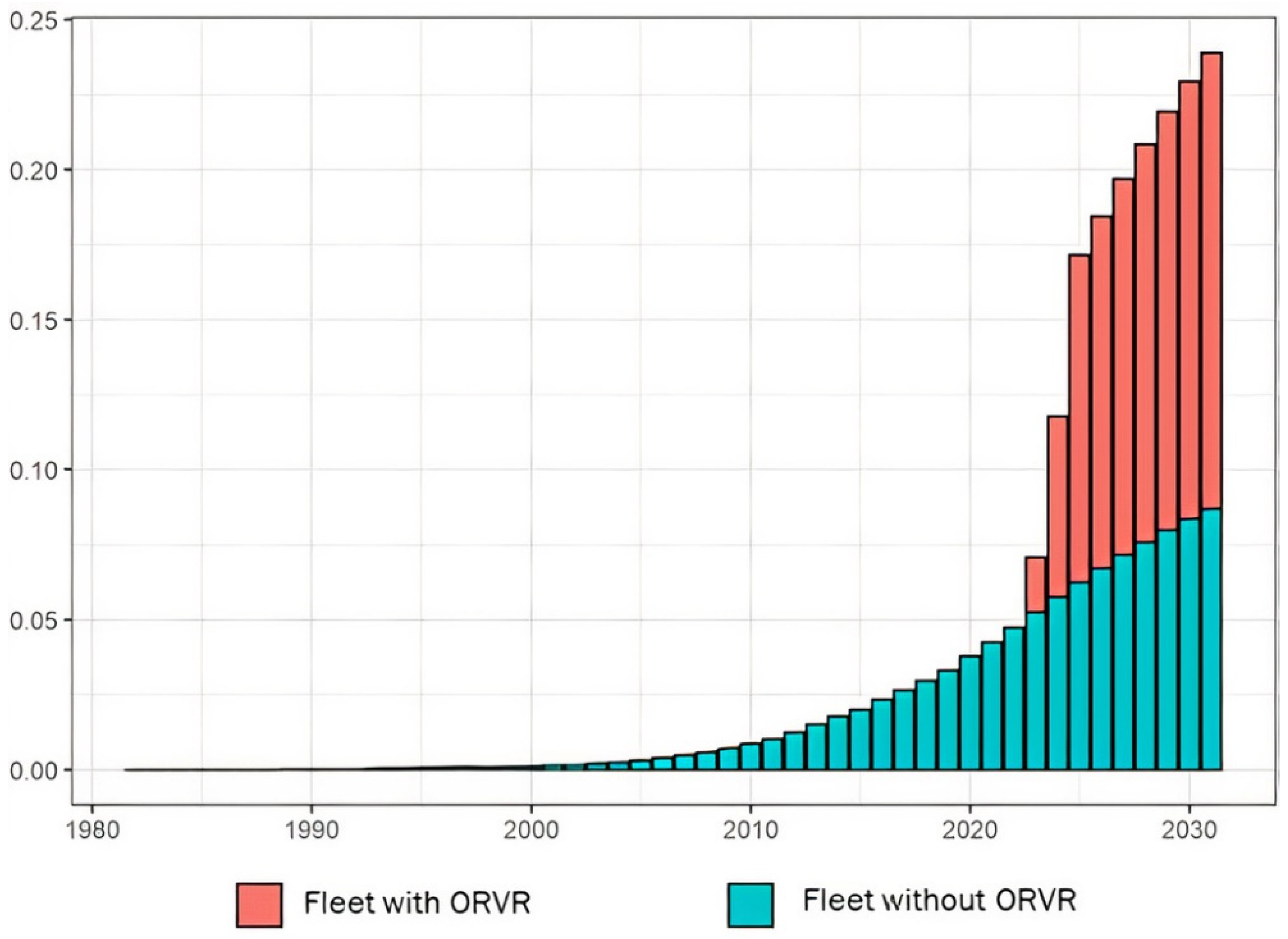
3.1. Vehicular Composition and Projections

The vehicle composition was updated based on information provided by São Paulo’s Secretariat of Infrastructure and Environment (SIMA) regarding the quantity of each type of fuel sold in the MASP. These data were made available from 2006 to 2017, and were used to better estimate the number of vehicles circulating using gasoline and ethanol, as well as diesel vehicles. We also used the fleet growth estimate provided by both DENATRAN and ANFAVEA for the year 2031. Figure 1 shows the projected fleet for Brazil from 1967 to 2031, while Figure 2 shows the fleet fraction of vehicles equipped with ORVR and those not equipped in 2031 for the year of use. The flow of vehicles was obtained with the information provided by the CET-SP and by the concessionaires that operate tolls in the region.

3.2. Emissions Estimations

Emissions from the transportation sector were estimated for Brazil. The estimated emissions by type of vehicles are shown in

Table 1. Vehicular emissions in Brazil by type of vehicle in 2011, 2015, 2018, and 2031 (t/year).

Vehicles	CO	NOX	PM2.5	SO2	CO2	Year
Total	900,000	750,000	18,000			2011 [26]
Total	8,864,014	1,722,666	79,594	10,195		2015 [27]
Bus	41,099	205,573	5130	1576	49,439,894	2018 (This Study)
LCV	54,668	31,613	1685	1034	37,133,594
MC	259,737	15,505	881	367	12,504,541
PC	319,925	29,967	336	1819	78,213,001
Trucks	58,744	350,836	10,129	2305	72,335,875
Total	734,172	633,493	18,162	7101	249,626,905
Bus	39,496	201,265	2987	573	89,818,049	2031 (This study)
LCV	46,623	38,982	1822	337	60,602,664
MC	319,676	14,264	1353	105	18,094,629
PC	228,625	14,530	466	488	104,287,669
Trucks	50,902	347,312	5586	834	130,809,267
Total	685,322	616,353	12,213	2337	403,612,277

Note: LCV represents light commercial vehicles, PC passenger cars, and MC motorcycles.

expressed as t/year. We added a comparison with the official vehicular emissions inventory from the Ministry of Environment for the year 2011 [26]. The comparison with the EDGAR inventory for transport during the year 2015 shows that CO estimates are 12 times higher than our estimations, NOX is 2.7 times higher, and PM2.5 4 times higher. The emissions of CO, non-methane hydrocarbons (NMHC), NO_X, and PM_2.5 align with the 2011 inventory in general, although CO and NO_X are slightly lower in our study. The main emitters of CO are passenger cars (PC), motorcycles (MC), and light commercial vehicles (LCV), while trucks and buses are more responsible for NO_X, PM_2.5, and SO₂. In the case of CO₂, PC and trucks are the main emitters. The projection for 2031 shows decreases in all pollutants, with the exception of CO₂, which will increase 61%.

Evaporative emissions for all scenarios are shown in

Table 2. NMHC emissions by type of vehicle and scenario in Brazil (t/year).

Scenario	Vehicles	Diurnal	Exhaust	Fueling Station	Fueling Vehicles	Hot Soak	Running Losses	Total
S0 2018	Bus	0	6430	0	0	0	0	6430
	LCV	314	5904	5223	5223	1324	464	18,454
	MC	1541	35,833	19,508	19,508	1878	958	79,225
	PC	2854	32,204	33,224	33,224	9161	3430	114,097
	Trucks	0	11,407	0	0	0	0	11,407
	Total	4709	91,778	57,955	57,955	12,363	4852	229,613
S1 2018	Bus	0	6430	0	0	0	0	6430
	LCV	314	5904	0	5223	1324	464	13,230
	MC	1541	35,833	0	19,508	1878	958	59,717
	PC	2854	32,204	0	33,224	9161	3430	80,873
	Trucks	0	11,407	0	0	0	0	11,407
	Total	4709	91,778	0	57,955	12,363	4852	171,657
S2 2018	Bus	0	6430	0	0	0	0	6430
	LCV	314	5904	0	522	1324	464	8530
	MC	1541	35,833	0	1951	1878	958	42,160
	PC	2854	32,204	0	3322	9161	3430	50,972
	Trucks	0	11,407	0	0	0	0	11,407
	Total	4709	91,778	0	5795	12,363	4852	119,499
S3 2031	Bus	0	3273	0	0	0	0	3273
	LCV	459	5048	0	9643	504	193	15,846
	MC	1534	38,030	0	32,282	474	185	72,504
	PC	3408	22,225	0	48,519	2353	894	77,398
	Trucks	0	6348	0	0	0	0	6348
	Total	5401	74,924	0	90,444	3331	1272	175,369
S4 2031	Bus	0	3273	0	0	0	0	3273
	LCV	196	5048	9643	4232	504	83	19,706
	MC	1534	38,030	32,282	32,282	474	80	104,682
	PC	1457	22,225	48,519	21,294	2353	384	96,232
	Trucks	0	6348	0	0	0	0	6348
	Total	3187	74,924	90,444	57,808	3331	547	230,241
S5 2031	Bus	0	3273	0	0	0	0	3273
	LCV	459	5048	0	964	504	193	7168
	MC	1534	38,030	0	3228	474	185	43,450
	PC	3408	22,225	0	4852	2353	894	33,731
	Trucks	0	6348	0	0	0	0	6348
	Total	5401	74,924	0	9044	3331	1272	93,970
S6 2031	Bus	0	3273	0	0	0	0	3273
	LCV	196	5048	0	1446	504	83	7277
	MC	1534	38,030	0	3228	474	80	43,346
	PC	1457	22,225	0	7278	2353	384	33,697
	Trucks	0	6348	0	0	0	0	6348
	Total	3187	74,924	0	11952	3331	547	93,941
S7 2031	Bus	0	3273	0	0	0	0	3273
	LCV	459	5048	9643	964	504	193	16,810
	MC	1534	38,030	32,282	3228	474	185	75,732
	PC	3408	22,225	48,519	4852	2353	894	82,250
	Trucks	0	6348	0	0	0	0	6348
	Total	5401	74,924	90,444	9044	3331	1272	184,413
S8 2031	Bus	0	3273	0	0	0	0	3273
	LCV	196	5048	9643	1446	504	83	16,920
	MC	1534	38,030	32,282	3228	474	80	75,628
	PC	1457	22,225	48,519	7278	2353	384	82,216
	Trucks	0	6348	0	0	0	0	6348
	Total	3187	74,924	90,444	11,952	3331	547	184,385
S9 2031	Bus	0	3273	0	0	0	0	3273
	LCV	459	5048	9643	9643	504	193	25,489
	MC	1534	38,030	32,282	32,282	474	185	104,785
	PC	3408	22,225	48,519	48,519	2353	894	125,917
	Trucks	0	6348	0	0	0	0	6348
	Total	5401	74,924	90,444	90,444	3331	1272	265,812

. Scenario S2, which considers Stage 1 + Stage 2, emits 119,498 (t/year), representing a 47.96% decrease in total HCNM compared to 2018. The decrease is due to reductions in emissions associated with supply, equivalent to 95%. In the case of Scenario 1 (without ORVR, with Stage 1, and without Stage 2) the reduction in this type of emission would be less, equal to 50%. For vehicle evaporative emissions projections for the year 2031, in the case of HCNM emissions, each scenario was compared with Scenario 9, which considers an HCNM estimate without any evaporative emissions control measures. Table 2 also shows 2031 HCNM vehicle emissions in Brazil, for each scenario. As Scenario 9 does not consider any measure to reduce evaporative emissions, all future scenarios are lower than this one. The future scenarios do not consider new emissions standards for exhaust emissions, and the reduction in these emissions is due to fleet change. Scenario 3 represents a decrease of 34.03%, S4 13.11%, S5 64.65%, S6 64.39%, S7 30.62%, and S8 30.36%, all in comparison with S9. Scenario 4, which consists of the implementation of only ORVR in the future, represents a considerable decrease in comparison to Scenario 0. In general, the most important emissions are due to fueling and exhaust.

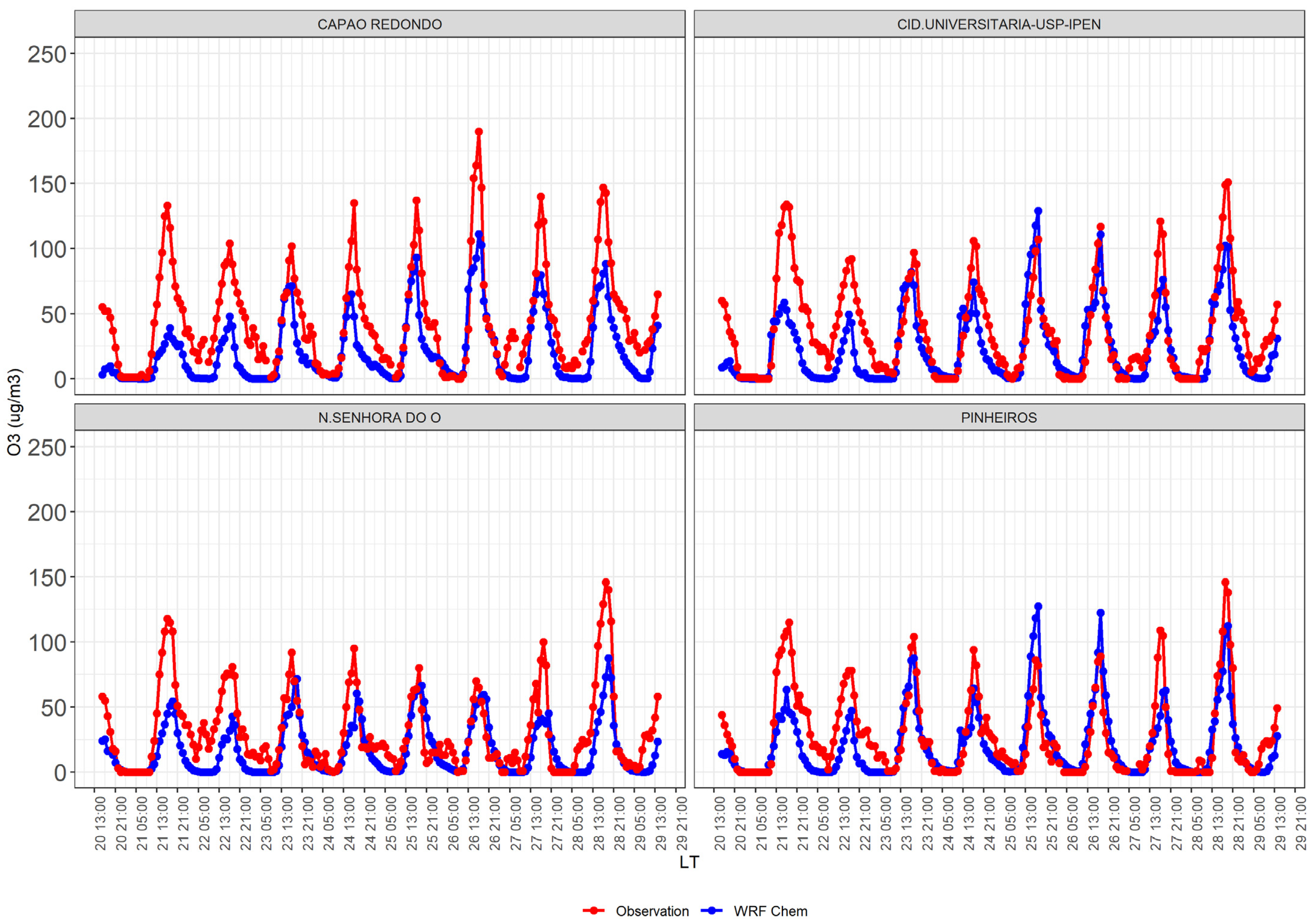
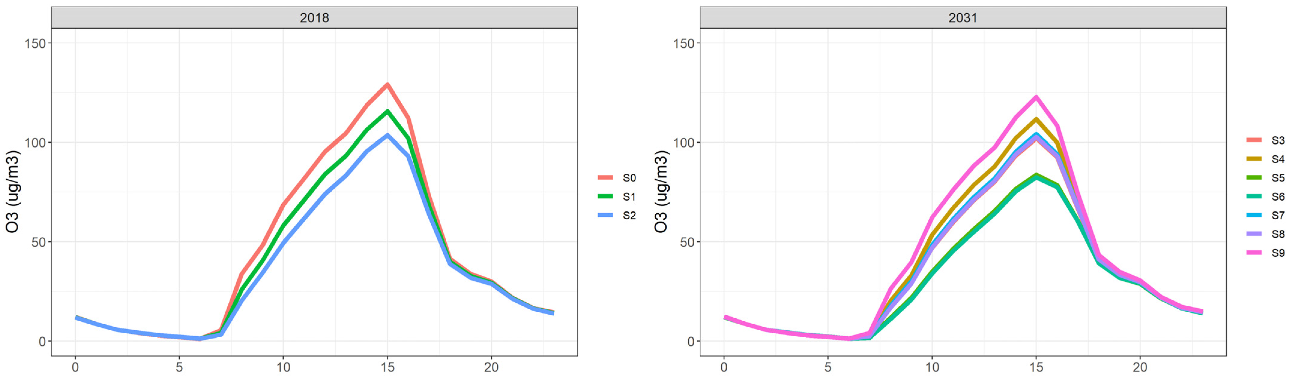
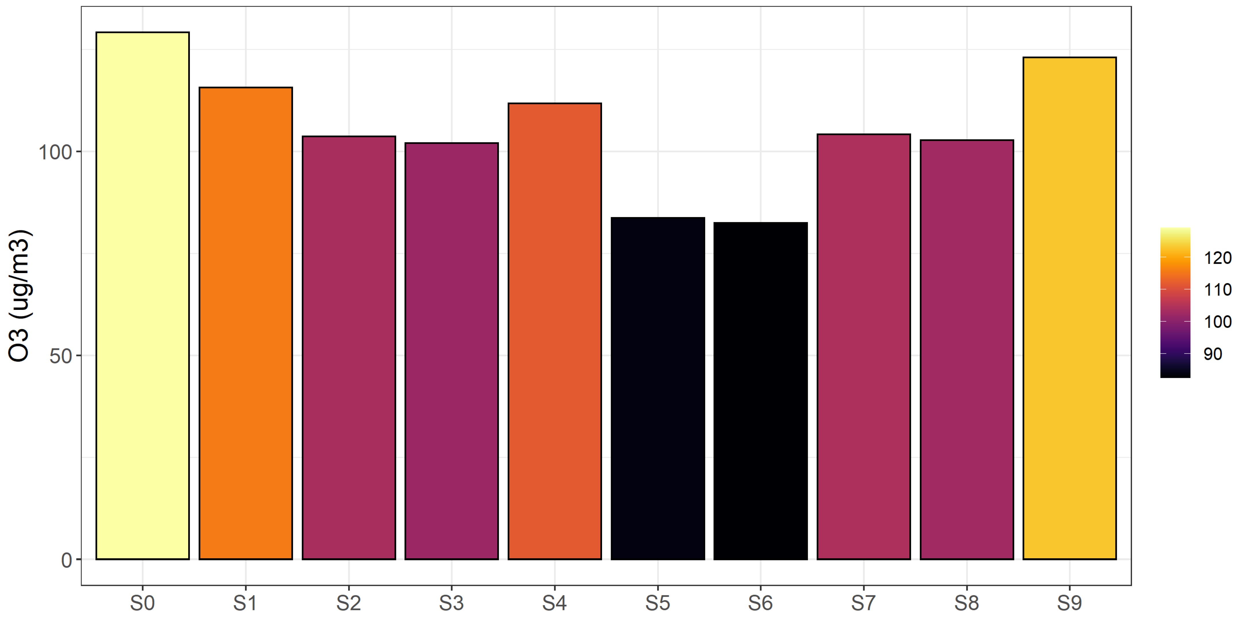
3.3. Air Quality Modeling

The meteorological simulation fields presented a very good agreement with observations especially for temperature and wind speed, as shown on Figures S1 and S2, and Table S1 (Supplementary Materials). Specifically, we found correlations above 0.9 for temperature and 0.7 for wind speed. As the main source of CO is vehicular emissions, having a good representation of the simulated concentrations of this gas is crucial to assess the inventory. Figure 3 shows the comparison between observations and simulations for CO concentrations (ppm) at CETESB stations of Parque D. Pedro II and Pinheiros. Our simulation has highest correlation for CO as 0.52, which means that the emissions estimation is reasonable, as is the diurnal and spatial representation. Similar results were found for other CETESB stations (not shown). In the same way, Figure 4 shows the results for NOx concentrations (μg/m³) for the stations Interlagos and Pinheiros. From these figures, we can see a very good agreement between modeled and observed values. Actually, the correlation values for NO_X were around 0.7 with the highest value of 0.82, which is fundamental for a good representation of ozone for two main reasons. First, a good representation of CO concentrations shows us that the vehicular emissions are relatively well represented in the model, with a diurnal cycle of emissions, including rush hours. Second, NO_x’s good performance will provide an appropriate base for the ozone precursors. These features contributed to the good representation of ozone concentrations, as one can see in Figure 5 for the stations of Capão Redondo, Cid.Universtiaria-USP-IPEN, Nossa Senhora do Ó and Pinheiros. The correlation values for O₃ values were around 0.75 with the highest value of 0.83 in stations Ibirapuera and Pinheiros. The results obtained for CO, NO_x, and O₃ give us confidence in the model’s results for analyzing the future scenarios proposed in this work.

Figure 6 shows the results for scenarios 0, 1, and 2 for the year 2018. The maximum hourly concentrations of the base scenario 2018 indicate that at 15:00, values of 129.14 µg/m³ were reached. The simulations show that the maximum ozone reductions in 2018 would be with Scenario 2 (Stage 1 + Stage 2), at 15:00, with 103.70 μg/m³, representing a decrease of 25.44 μg/m³. This indicates that controlling evaporative emissions in the MASP is an efficient way to reduce ozone concentrations. When we compare all the scenarios for 2031, shown in Figure 6, it is observed that, on average, the biggest difference from Scenario 9 (L7 without ORVR, without Stage 1, and without Stage 2), which was considered as a reference scenario for the most adequate representation of the vehicle fleet that year, occurs in Scenario 6 (L7 with ORVR with Stage 1 and with Stage 2, in 2031) which reaches the value of 82.43 μg/m³, followed by Scenario 5 (L7 without ORVR, with Stage 1, and Stage 2, in 2031) with 83.72 µg/m³, which represents an average decrease in both scenarios of 39.92 μg/m³. The comparison of the Wilcoxon test between all hourly data in Scenarios 5 and 6 shows that there are no significant differences between these two scenarios, both presenting practically the same efficiency in reducing ozone concentrations.

Figure 7 shows the maximum ozone concentrations for each scenario. It appears that Scenarios 1 and 2 of the year 2018 have lower concentrations than the base Scenario 0. The lowest reduction is found in Scenario 2, which corresponds to 2018 base L6 without ORVR, with Stage 1 and Stage 2, indicating that to reduce short-term ozone concentrations, an excellent alternative would be the introduction of Stages 1 and 2. The scenario that provides the lowest concentrations of ozone in the year 2031 is C6 (L7 with ORVR, with Stage 1, with Stage 2, in 2031) with 82.43 μg/m³ followed by scenario C5 (L7 without ORVR, with Stage 1, with Stage 2, in 2031) with 82.71 μg/m³. HCNM emissions in both scenarios are quite similar, resulting in similar concentrations. The main difference consists of the spatial distribution of the sources because, with Scenario 5, the reductions happen only at the filling stations, but with Scenario 6 they happen at the stations and also in the entire road network by vehicles with ORVR (leading to lower “diurnal” and “running loss” emissions contributions).

Figure 8 shows the mean difference of O₃ concentrations (%) for the year 2031 between Scenarios S9 and S5. We can see that Scenario S5 will contribute to an O₃ reduction of around 25% in west MASP. The spatial distribution of this reduction follows the local circulation which characterizes MASP. In particular, MASP is under influence of sea-breeze, cold fronts, and other atmospheric systems which transport MASP pollutants [28,29,30], being very common the situation where higher concentrations are observed away from air pollutant sources.

4. Discussion

In this study, we have performed a vehicular emissions inventory for an important region of Brazil, selecting the metropolitan area of São Paulo, MASP, to spatially allocate emissions. The comparison between emissions shows that the official inventory for Brazil in 2011 has similar values with our estimation, with ratios of 1.2 and 1.18 higher for CO and NO_X, respectively, than our estimation for 2018, while the ratio for PM2.5 is 1. Our inventory considered the effect of fleet turnover and the newer emission standard L6 in 2014 for light vehicles, equivalent to Euro 5, and P7 for heavy vehicles in 2012, equivalent with Euro 5 [18,31]. Consequently, it is reasonable to expect that the transportation emissions in 2018 will be lower than in the year 2011, despite fleet growth. Actually, the CETESB inventory also has presented lower transportation emissions in recent years for MASP. Furthermore, as recommended by the European Emissions Guidelines [32], our inventory presents a fleet calibrated with fuel consumption. This means that our estimation of fuel consumption matches transportation fuel sales, resulting in more confident results. Nevertheless, there are areas for improvement. VEIN incorporates the raw emission factors from CETESB and also options to adjust the factors by tunnel measurements made in São Paulo [3]. Recently it was added an experimental feature to include the effect of inspection and maintenance programs into VEIN to account for high emitter vehicles in circulation, following the approaches implemented in the models MOBILE 6.2 and MOVES [33]. In summary, although our estimation provides confidence and reliability, there is still a need to improve the estimation in emission factors and future research and measurements are necessary.

Currently, there are no systems to control evaporative emissions for refueling in Brazil yet. The planned introduction of emissions standard PROCONVE L7 aims at a reduction in evaporative emissions without indicating a specific device or technology. Thus, our study aims to provide critical information to decisionmakers about different scenarios to control these emissions with ORVR or Stage 2 devices in the present and future scenarios. Different scenarios were designed based on the literature review. Obviously, assumptions are needed regarding the efficiency of the control devices. However, we provide information that, despite ORVR controlling diurnal and refueling emissions, this system would take a timespan longer than 2031 to efficiently decrease evaporative emissions and consequently reduce ozone concentrations.

We ran air quality models to study the contribution of evaporative emissions to ozone concentrations. Specifically, we used the WRF-Chem model with a grid spacing of 3 km to represent local circulations. We used the meteorological conditions of 2018 and changed emissions to represent different scenarios for the years 2018 and 2031. While we consider that the comparison between observed and simulated concentrations was satisfactory, we do know that a comprehensive emissions inventory would improve the correlations and reduce bias. Currently, the authors are developing a multi-year emissions inventory for Brazil with a monthly resolution, which will further allow an explanation of the responsibility of transportation emissions for air quality. A recently published manuscript explains that at city centers, local emissions are more responsible [34]. This has been corroborated in Brazil, where small cities in the northwest part of São Paulo are impacted by external sources of air pollution producing high levels of O₃ [30], as shown in Figure 7. This is also important for biomass burning [35]. Furthermore, despite the needed improvement in emissions inventories, more research is necessary to better represent the meteorological conditions. For instance, a recent manuscript shows that updating land-use improves the performance of WRF simulation considerably [36].

5. Conclusions

The simulations for the base year 2018 show a good agreement between the simulated and observed concentrations for most air quality monitoring stations. The results obtained for scenarios 1 and 2 show that the implementation of Stages 1 and 2 reduces HCNM emissions by 47.96%. As a result, there is an average reduction of 19.9% in the average concentrations of tropospheric ozone.

For the year 2031, when we consider all scenarios, 3, 4, 5, 6, 7, and 8, we can see a reduction in HCNM emissions of 34.03%, 13.11%, 64.65%, 64.39%, 30.62%, and 30.36% in comparison with Scenario 9, which translates into maximum reductions in ozone concentrations of 17.01% (20.92 µg/m³), 9.14% (11.24 µg/m³), 31.93% (39.27 µg/m³), 32.98% (40.55 µg/m³), 15.33% (18.85 µg/m³), and 16.42% (20.19 µg/m³), between 12 and 16:00, respectively. However, the reductions in Scenarios 4 and 7 are the least significant, as demonstrated by the Wilcoxon test (p = 0.05203). In conclusion, the scenarios that show the greatest reductions in ozone concentrations are Scenario 5: Base L7 (Shed 0.5 48 h) without ORVR, with Stage 1, with Stage 2 (fleet 2031), and Scenario 6: Base L7 (Shed 0.5 48 h) with ORVR, with Stage 1, with Stage 2 (fleet 2031). The Wilcoxon test was applied between the hourly concentrations of Scenarios 5 and 6 without significant differences being found (p > 0.05), both scenarios being equivalent in terms of efficiency. Despite the ORVR controlling “diurnal” evaporative emissions at filling stations for vehicles, the use of this device in conjunction with the control performed by Stage 2 produces a 5% loss of efficiency as estimated in this work, having considered the scenarios that contemplated an 85% combination efficiency for Stage 2 contributing to a relative increase in hydrocarbon emissions, when compared to the use of systems alone. For the simulations carried out in this study, the evaporative emissions existing in the distribution networks were not considered during the transfer of fuel to the tank trucks that supply the gas stations.

References

1. Departamento Nacional del Transito. (Denatran) Frota Nacional (2017); Goverdo Federal do Brasil. 2017. Available online: https://www.gov.br/infraestrutura/pt-br/assuntos/transito/conteudo-denatran/frota-de-veiculos-2017 (accessed on 21 December 2021).
2. Landrigan, P.J.; Fuller, R.; Acosta, N.J.R.; Adeyi, O.; Arnold, R.; (Nil) Basu, N.; Baldé, A.B.; Bertollini, R.; Bose-O’Reilly, S.; Boufford, J.I.; et al. The Lancet Commission on pollution and health. Lancet 2018, 391, 462–512. [Google Scholar] [CrossRef] [Green Version]
3. Nogueira, T.; Kamigauti, L.; Pereira, G.; Gavidia-Calderón, M.; Ibarra-Espinosa, S.; de Oliveira, G.; Miranda, R.; Vasconcellos, P.; Freitas, E.; Andrade, M. Evolution of Vehicle Emission Factors in a Megacity Affected by Extensive Biofuel Use: Results of Tunnel Measurements in São Paulo, Brazil. Environ. Sci. Technol. 2021, 55, 6677–6687. [Google Scholar] [CrossRef] [PubMed]
4. Juráň, S.; Grace, J.; Urban, O. Temporal Changes in Ozone Concentrations and Their Impact on Vegetation. Atmosphere 2021, 12, 82. [Google Scholar] [CrossRef]
5. Zapletal, M.; Juran, S.; Krpes, V.; Michna, K.; Cudlin, P.; Edwards, M. Effect of ozone flux on selected structural and antioxidant characteristics of a mountain norway spruce forest. Balt. For. 2018, 24, 261–267. [Google Scholar]
6. Di, Q.; Dai, L.; Wang, Y.; Zanobetti, A.; Choirat, C.; Schwartz, J.D.; Dominici, F. Association of Short-term Exposure to Air Pollution With Mortality in Older Adults. JAMA 2017, 318, 2446–2456. [Google Scholar] [CrossRef] [PubMed]
7. Ibarra-Espinosa, S.; Dias de Freitas, E.; Ropkins, K.; Dominici, F.; Rehbein, A. Negative-Binomial and quasi-poisson regressions between COVID-19, mobility and environment in São Paulo, Brazil. Environ. Res. 2021, 204, 112369. [Google Scholar] [CrossRef] [PubMed]
8. CETESB. Qualidade do ar no Estado de São Paulo; Companhia Ambiental do Estado de São Paulo: São Paulo, Brazil, 2017.
9. De Andrade, M.F.; Ynoue, R.Y.; Freitas, E.D.; Todesco, E.; Vara Vela, A.; Ibarra, S.; Martins, L.D.; Martins, J.A.; Carvalho, V.S.B. Air quality forecasting system for Southeastern Brazil. Front. Environ. Sci. 2015, 3, 9. [Google Scholar] [CrossRef] [Green Version]
10. Andrade, M.F.; Fornaro, A.; Freitas, E.D.; Mazzoli, C.R.; Martins, L.D.; Boian, C.; Oliveira, M.G.L.; Peres, J.; Carbone, S.; Alvalá, P.; et al. Ozone sounding in the Metropolitan Area of São Paulo, Brazil: Wet and dry season campaigns of 2006. Atmos. Environ. 2012, 61, 627–640. [Google Scholar] [CrossRef]
11. Schuch, D.; Freitas, E.D.; Espinosa, S.I.; Martins, L.D.; Carvalho, V.S.B.; Ramin, B.F.; Silva, J.S.; Martins, J.A.; Andrade, M.F. A two decades study on ozone variability and trend over the main urban areas of the São Paulo state, Brazil. Environ. Sci. Pollut. Res. 2019, 26, 31699–31716. [Google Scholar] [CrossRef] [PubMed] [Green Version]
12. Mellios, G.; Ntziachristos, L. EMEP/EEA Emission Inventory Guidebook; Gasoline Evaporation from Vehicles; European Environmental Agency: Copenhagen, Denmark, 2016. Available online: https://www.eea.europa.eu/themes/air/air-pollution-sources-1/emep-eea-air-pollutant-emission-inventory-guidebook/emep (accessed on 21 December 2021).
13. De Gennaro, M.; Paffumi, E.; Martini, G. Data-driven analysis of the effectiveness of evaporative emissions control systems of passenger cars in real world use condition: Time and spatial mapping. Atmos. Environ. 2016, 129, 277–293. [Google Scholar] [CrossRef]
14. CONAMA. Resolução Conama 018/1986; Governo do Brasil: Brasilia, Brazil, 1986.
15. Carvalho, V.S.B.; Freitas, E.D.; Martins, L.D.; Martins, J.A.; Mazzoli, C.R.; de Fátima Andrade, M. Air quality status and trends over the Metropolitan Area of São Paulo, Brazil as a result of emission control policies. Environ. Sci. Policy 2015, 47, 68–79. [Google Scholar] [CrossRef]
16. Pérez-Martínez, P.J.; de Fátima Andrade, M.; de Miranda, R.M. Traffic-related air quality trends in São Paulo, Brazil. J. Geophys. Res. Atmos. 2015, 120, 6290–6304. [Google Scholar] [CrossRef] [Green Version]
17. CONAMA. Resolução Conama 492; Governo do Brasil: Brasilia, Brazil, 2018.
18. Ibarra-Espinosa, S.; Ynoue, R.; O’Sullivan, S.; Pebesma, E.; Andrade, M.D.F.; Osses, M. VEIN v0.2.2: An R package for bottom-up vehicular emissions inventories. Geosci. Model Dev. 2018, 11, 2209–2229. [Google Scholar] [CrossRef]
19. Ibarra-Espinosa, S.; Ynoue, R.; Giannotti, M.; Ropkins, K.; de Freitas, E.D. Generating traffic flow and speed regional model data using internet GPS vehicle records. MethodsX 2019, 6, 2065–2075. [Google Scholar] [CrossRef] [PubMed]
20. Ibarra-Espinosa, S.; Ynoue, R.Y.; Ropkins, K.; Zhang, X.; de Freitas, E.D. High spatial and temporal resolution vehicular emissions in south-east Brazil with traffic data from real-time GPS and travel demand models. Atmos. Environ. 2020, 222, 117136. [Google Scholar] [CrossRef]
21. CETESB. Emissões Veiculares no Estado de São Paulo 2018; Companhia Ambiental do Estado de São Paulo: São Paulo, Brazil, 2019.
22. Grell, G.A.; Peckham, S.E.; Schmitz, R.; McKeen, S.A.; Frost, G.; Skamarock, W.C.; Eder, B. Fully coupled “online” chemistry within the WRF model. Atmos. Environ. 2005, 39, 6957–6975. [Google Scholar] [CrossRef]
23. Ibarra-Espinosa, S.; Schuch, D.; de Freitas, E. Eixport: An R package to export emissions to atmospheric models. J. Open Source Softw. 2018, 3, 6071–6074. [Google Scholar] [CrossRef]
24. Fung, F.; Maxwell, B. Onboard Refueling Vapor Recovery: Evaluation of the ORVR Program in the United States; ICCT: Washington, DC, USA, 2011. [Google Scholar]
25. US-EPA. AP42. Chapter 5.2. Transportation and Marketing of Petroleum Liquids; US-EPA, Research Triangle Park: Washington, DC, USA, 2008.
26. MMA. 1o Inventário Nacional de Emissões Atmosféricas por Veículos Automotores Rodoviários; Governo do Brasil: Brasilia, Brazil, 2011.
27. EJ-JRC/PBL Emission Database for Global Atmospheric Research (EDGAR), Release EDGAR v4.3.1_v2 (1970–2010); JRC: Brussels, Belgium, 2016.
28. Freitas, E.D.; Rozoff, C.M.; Cotton, W.R.; Dias, P.L.S. Interactions of an urban heat island and sea-breeze circulations during winter over the metropolitan area of São Paulo, Brazil. Bound. Layer Meteorol. 2007, 122, 43–65. [Google Scholar] [CrossRef]
29. Nair, K.N.; Freitas, E.D.; Sánchez-Ccoyllo, O.R.; Silva Dias, M.A.F.; Silva Dias, P.L.; Andrade, M.F.; Massambani, O. Dynamics of urban boundary layer over São Paulo associated with mesoscale processes. Meteorol. Atmos. Phys. 2004, 86. [Google Scholar] [CrossRef]
30. Squizzato, R.; Nogueira, T.; Martins, L.D.; Martins, J.A.; Astolfo, R.; Machado, C.B.; Andrade, M.F.; Freitas, E.D. Beyond megacities: Tracking air pollution from urban areas and biomass burning in Brazil. NPJ Clim. Atmos. Sci. 2021, 4, 17. [Google Scholar] [CrossRef]
31. CETESB. Emissões Veiculares no Estado de São Paulo 2019; Companhia Ambiental do Estado de São Paulo: São Paulo, Brazil, 2020.
32. Ntziachristos, L.; Samaras, Z. EMEP/EEA Emission Inventory Guidebook, Road Transport: Passenger Cars, Light Commercial Trucks, Heavy-Duty Vehicles Including Buses and Motorcycles; European Environment Agency: Copenhagen, Denmark, 2016.
33. Koupal, J.; Cumberworth, M.; Michaels, H.; Beardsley, M.; Brzezinski, D.J. Design and Implementation of MOVES: EPA‘s New Generation Mobile Source Emission Model. Ann Arbor 2003, 1001, 48105. [Google Scholar]
34. Thunis, P.; Clappier, A.; de Meij, A.; Pisoni, E.; Bessagnet, B.; Tarrason, L. Why is the city’s responsibility for its air pollution often underestimated? A focus on PM2.5. Atmos. Chem. Phys. 2021, 21, 18195–18212. [Google Scholar] [CrossRef]
35. Vara-Vela, A.; de Fátima Andrade, M.; Zhang, Y.; Kumar, P.; Ynoue, R.Y.; Souto-Oliveira, C.E.; da Silva Lopes, F.J.; Landulfo, E. Modeling of Atmospheric Aerosol Properties in the São Paulo Metropolitan Area: Impact of Biomass Burning. J. Geophys. Res. Atmos. 2018, 123, 9935–9956. [Google Scholar] [CrossRef]
36. Pedruzzi, R.; Andreão, W.L.; Baek, B.H.; Hudke, A.P.; Glotfelty, T.W.; Dias de Freitas, E.; Martins, J.A.; Bowden, J.H.; Pinto, J.A.; Alonso, M.F.; et al. Update of land use/land cover and soil texture for Brazil: Impact on WRF modeling results over São Paulo. Atmos. Environ. 2022, 268, 118760. [Google Scholar] [CrossRef]
Figure 1. Total vehicle fleet projected for Brazil (millions) with data from DENATRAN and growth estimates reported by ANFAVEA.
Atmosphere 13 00082 g001
Figure 2. Fraction of the fleet of light vehicles in circulation (excluding scrapped vehicles) with and without ORVR in the year 2031.
Atmosphere 13 00082 g002
Figure 3. Concentrations of CO (ppm) for the stations Cerqueira Cesar, Marg. Tietê-Pte Remedios, Parque D. Pedro II and Pinheiros during April 2018.
Atmosphere 13 00082 g003
Figure 4. Concentrations of NOX (μg/m3) for the stations Capão Redondo, Cerqueira Cesar, Interlagos and Pinheiros during April 2018.
Atmosphere 13 00082 g004
Figure 5. Concentrations of O3 (μg/m3) for the stations Capão Redondo, Cid. Universitaria-USP-IPEN, N.Senhora de O and Pinheiros during April 2018.
Atmosphere 13 00082 g005
Figure 6. O3 (μg/m3) concentrations for scenarios in 2018 and 2031. Note that the meteorology of 2018 was used and the scenarios in 2031 are based on the emissions projected for the year 2031.
Atmosphere 13 00082 g006
Figure 7. Maximum hourly O3 (μg/m3) concentrations for each scenario between 12:00 and 16:00 local time.
Atmosphere 13 00082 g007
Figure 8. Average difference of O3 (%) between scenarios S9 and S5 between 12:00 and 16:00 local time.
Atmosphere 13 00082 g008