Article

A Fast-Converging Kernel Density Estimator for Dispersion in Horizontally Homogeneous Meteorological Conditions

Department of Mechanical Engineering, KU Leuven, Celestijnenlaan 300, BE-3001 Leuven, Belgium
*
Author to whom correspondence should be addressed.
Atmosphere 2021, 12(10), 1343; https://doi.org/10.3390/atmos12101343
Submission received: 13 July 2021 / Revised: 7 October 2021 / Accepted: 9 October 2021 / Published: 14 October 2021
(This article belongs to the Special Issue Air Pollution Modelling)

Abstract

:
Kernel smoothers are often used in Lagrangian particle dispersion simulations to estimate the concentration distribution of tracer gasses, pollutants etc. Their main disadvantage is that they suffer from the curse of dimensionality, i.e., they converge at a rate of 4 / ( d + 4 ) with d the number of dimensions. Under the assumption of horizontally homogeneous meteorological conditions, we present a kernel density estimator that estimates a 3D concentration field with the faster convergence rate of a 1D kernel smoother, i.e., 4 / 5 . This density estimator has been derived from the Langevin equation using path integral theory and simply consists of the product between a Gaussian kernel and a 1D kernel smoother. Its numerical convergence rate and efficiency are compared with that of a 3D kernel smoother. The convergence study shows that the path integral-based estimator has a superior convergence rate with efficiency, in mean integrated squared error sense, comparable with the one of the optimal 3D Epanechnikov kernel. Horizontally homogeneous meteorological conditions are often assumed in near-field range dispersion studies. Therefore, we illustrate the performance of our method by simulating experiments from the Project Prairie Grass data set.

1. Introduction

In atmospheric dispersion modeling, one describes the transport of tracer gasses or other scalar quantities under given meteorological conditions and release characteristics. A Lagrangian approach is often used to model atmospheric dispersion. In this approach, a stochastic differential equation (SDE) describes the trajectories of the pollutant particles. The objective is to obtain the distribution of the particle positions from this SDE. Usually, such a distribution cannot be obtained analytically and consequently, a numerical procedure is required to estimate the distribution from a finite number of particle positions. Nonparametric density estimation has the advantage that no pre-specified functional form for the distribution is assumed. Examples of such methods are histograms, orthogonal series estimators, restricted maximum likelihood estimators, etc. A discussion about the different methods can be found in [1]. The selection of a proper method depends on the expected complexity of the distribution and the dimensionality of the data. In particular, we will focus on the kernel smoothing approach [2,3].
Kernel smoothers have a long tradition of being used in atmospheric dispersion modeling. Since [4] introduced them into this field, several models have incorporated them over the course of time, e.g., [5,6,7]. Kernel smoothers offer a good trade-off between complexity and performance. Since they are relatively simple to analyze mathematically, their mathematical properties are well known. The performance of kernel smoothers is mesh independent because of the pointwise convergence. They also use data quite efficiently. This is illustrated by the fact that kernel smoothers converge faster than histograms ([8], Section 2.8, p. 36). A vast amount of literature is dedicated to the optimal performance of kernel smoothers. In particular, an overview of bias and variance reduction techniques can be found in [9]. Such techniques have a solely mathematical foundation, i.e., they are formulated independently of the way the data were obtained. In case of physical applications, however, the model that generates the data may yield extra information about the underlying density. This information can also be used to improve the performance of the kernel smoother. Despite the available computer power today, the development of fast-converging kernel density estimators is still a topical research subject in atmospheric dispersion modeling (see, e.g., [10]).
In this paper, a kernel estimator for dispersion in horizontally homogeneous meteorological conditions will be derived from the Langevin equation, which converges for a 3D concentration field as fast as a 1D kernel smoother would do for a 1D field. Botev et al. [11] proposed an adaptive kernel density estimation method based on the smoothing properties of linear diffusion processes. This method requires the numerical solution of a diffusion equation, which will increase the computational cost considerably in three dimensions. We use a completely different approach by resorting to path integral theory [12]. This allows us to derive a kernel density estimator from the 3D Langevin equation, which simply consists of the product between a Gaussian kernel and a kernel smoother. Alvarez et al. [13] present a path integral formalism for oceanic dispersion as an alternative to Lagrangian simulation. The main difference with our approach is that we calculate the horizontal particle coordinates from the vertical coordinates such that we only have to integrate over the vertical to obtain the 3D concentration field. This dimension reduction idea also forms the cornerstone of the particle-puff approach in [14] and our methodologies are similar. Although, the current work provides a rigorous mathematical argument for the method in terms of path integrals and extends it to the more general kernel smoother framework. Moreover, its convergence behavior is also discussed. The presented path integral-based method is not restricted to a process governed by the Langevin equation, but can be applied to any diffusion process. It also offers the flexibility to choose the kernel shape and bandwidth selection method for the involved kernel smoother freely.
In Section 2, the path integral-based kernel density estimator is presented as well as the kernel-smoothing framework. In Section 3.1, the superior convergence of the path integral-based estimator w.r.t. a classical 3D kernel smoother is numerically verified. The Project Prairie Grass dispersion experiment is simulated to demonstrate the method in Section 3.2. Section 4 provides a discussion of the results. Finally, Section 5 concludes the paper.

2. Methodology

The essence of dispersion modeling is to simulate the concentration field due to a pollutant source. In this work, we make the assumption of a point source at location x 0 R 3 . Then, it can be shown that the resulting concentration field c (kg m−3) at time t can be characterized as [15]
c ( t , x ) = t 0 t Q ( τ ) p ( t , x | τ , x 0 ) d τ , x R 3 ,
where t 0 denotes the start time of the release ( s ) and Q the source strength (kg s−1). The function p ( t , x | t , x ) is the transition probability density function (e.g., [16], Section 2.4, p. 68) of the stochastic process ( X t ) t > 0 that describes the trajectories of the pollutant particles. The density p gives the probability that a particle is situated in an infinitesimal volume d x around location x at time t given an earlier position ( t , x ) with t t .
The process ( X t ) t > 0 can be modeled by a stochastic differential equation. We choose the Langevin equation since it describes near-field range dispersion more accurately than the diffusion equation, e.g., [17]. The Langevin equation is commonly separated into two first-order differential equations: one describes the particle displacement and the other one the turbulent component of the particle velocity. Under the assumption of local Gaussian turbulence, these are given by
X ˙ t = u ( X t ; Φ ) + R ( Φ ) U t ,
U t ˙ = diag { α ( X t ) } U t + a ( Z t , W t ) e ^ w + diag { b ( X t ) } W ˙ t ,
with X t R 3 the particle position ( m ) at time t, u = ( u , v , w ) R 3 the mean background velocity (m s−1), U t = ( U t , V t , W t ) R 3 the particle-velocity noise vector (m s−1), W t R 3 the three-dimensional Wiener process, e ^ w = ( 0 , 0 , 1 ) the unit vector in the vertical direction and
R ( ϕ ) = cos ϕ sin ϕ 0 sin ϕ cos ϕ 0 0 0 1
a rotation matrix that accounts for the wind direction ϕ ( ). Further, the components of U t are oriented such that U t and V t are aligned with the streamwise and crosswind direction with resp. to ϕ = 0 and W t points in the vertical direction. In the following, time derivatives are notated by the dot notation, i.e., d X t = X ˙ t d t and d 2 X t = X ¨ t d t 2 . Typically, a stochastic variable will be notated by a capital letter and the corresponding state space variable by a lower case letter. The functions u , α , b : R 3 R 3 and a : R 2 R are given by classical relations for the atmospheric surface layer and can be found in Appendix A. In the current work, we assume that the meteorology is stationary. This assumption avoids the technicality that is inherent to a time-varying wind direction distribution, but the presented method can be further extended.
Equation (1) implies that the problem of determining the concentration field c comes down to determining the density p if the source is known. This can be achieved if a kernel representation of p is found.

2.1. Kernel Smoothing

The oldest, but still widely used, nonparametric density estimator is the histogram, which converges at a rate of 2 / ( d + 2 ) ([8], Section 2.8, p. 36) with d the dimension of the problem. Kernel smoothers, however, have a uniformly faster convergence rate for all d (see below). One can show that for any bounded, compactly supported function K : R d R satisfying
R d K ( x ) d x = 1 , R d x K ( x ) d x = 0 , x x K ( x ) d x = μ 2 ( K ) I ,
where I R d × d is the identity matrix and μ 2 ( K ) : = R d x i 2 K ( x ) d x is independent of i ( i = 1 , , d ), the following relationship holds (e.g., [8], Section 2.6, p. 32)
E [ p ^ ( t , x ; h ) ] = p ( t , x | t , x 0 ) + h 2 2 μ 2 ( K ) 2 p ( t , x | t , x 0 ) + o ( h 2 ) , h 0 .
Here, E [ · ] is the expectation value and the estimator
p ^ ( t , x ; h ) = 1 n p h d i = 1 n p K x X t ( i ) h , x R d ,
has been obtained by applying the strong law of large numbers. Further, 2 is the Laplacian, h R 0 + the bandwidth, n p the number of particles released at time t and X t ( i ) independent stochastic variables with image in R 3 and with distribution p ( t , · | t , x 0 ) that describes a particle’s location. The variables X t ( i ) are obtained by solving Equations (2) and (3). According to Equation (5), p ^ ( t , · ; h ) is an estimator for p ( t , · | t , x 0 ) . The functions K satisfying the above requirements are called kernel smoothers.
In order to measure how closely p ^ approximates p, the mean integrated squared error (MISE) can be used, i.e.,
MISE { p ^ ( t , · ; h ) } = R d E { p ^ ( t , x ; h ) p ( t , x | t , x 0 ) } 2 d x .
One can show that the optimal bandwidth h * that minimizes the asymptotic MISE satisfies ([8], Section 2.7, p. 35)
h * = R ( K ) d μ 2 ( K ) 2 { 2 p ( t , x | t , x 0 ) } 2 d x n p 1 / ( d + 4 ) , R ( K ) = R d K ( x ) 2 d x ,
with d the dimension of the problem. Consequently, inf h > 0 MISE { p ^ ( t , · ; h ) } = O ( n p 4 / ( d + 4 ) ) . The convergence rate 4 / ( d + 4 ) arises, because it can be shown that
MISE { p ^ ( t , · ; h ) } = R d Var { p ^ ( t , x ; h ) } + Bias 2 { p ^ ( t , x ; h ) } d x
in which the integrated variance and integrated squared bias are of order o ( n p 1 h d ) and o ( h 4 ) , n p , h 0 resp ([8], Section 2.5, p. 28, Section 2.9, p. 37).
If h * is substituted for h in Equation (9) with
Var { p ^ ( t , x ; h ) } = n p 1 h d R ( K ) p ^ ( t , x ; h ) + o n p 1 h d , n p , h 0 ,
and the bias provided by Equation (5), then the factor
C d ( K ) = { R ( K ) 4 μ 2 ( K ) 2 d } 1 / ( d + 4 ) ,
which only depends on the kernel K, can be separated in MISE { p ^ ( t , · ; h * ) } . The smaller C d ( K ) , the closer MISE { p ^ ( t , · ; h * ) } is to zero for a low amount of particles. Therefore, C d ( K ) is also referred to as the efficiency of the kernel K. One can show that the kernel smoother K * that minimizes (10) is the so-called Epanechnikov kernel ([18], Section 6.1, pp. 82–83), i.e.,
K d * ( x ) = π d / 2 Γ d 2 + 2 1 x x H 1 x x , x R d ,
with Γ ( · ) the gamma and H ( · ) the Heaviside function.
In order to determine the optimal bandwidth, the expressions
μ 2 K d * = 1 d + 4 , R K d * = 4 π d / 2 ( d + 4 ) Γ d 2 + 2 ,
need to be inserted in Equation (8). Only { 2 p ( t , x | t , x 0 ) } 2 d x then still needs to be determined. Unfortunately, this expression is unknown. A pragmatic way to deal with this issue is by replacing p with a normal distribution. Typically, one assumes that the variances in all directions are equal. In this work, we allow them to be different. Denote φ ( x ) with x R d the d-dimensional standard normal density function and Σ = diag { σ 1 2 , , σ d 2 } the covariance matrix with σ k 2 the variance in the k-th coordinate direction. One can verify that
R d | Σ | 1 / 2 2 φ Σ 1 / 2 x 2 d x = | Σ | 1 / 2 R d φ ( x ) 2 k = 1 d ( x k 2 1 ) σ k 2 2 d x = 1 2 π | Σ | R d 1 φ ( x ) 2 k = 2 d ( x k 2 1 ) σ k 2 1 2 σ 1 2 2 d x + | Σ | 1 / 2 2 σ 1 4 1 2 π d
with | · | the determinant. Proceeding by induction over the dimensions of the domain leads to the formula
R d | Σ | 1 / 2 2 φ Σ 1 / 2 x 2 d x = k = 1 d σ k 1 1 2 π d 1 2 k = 1 d σ k 4 + 1 4 k = 1 d σ k 2 2 ,
which we substitute for { 2 p ( t , x | t , x 0 ) } 2 d x in Equation (8). Note that if the variances in all directions are equal, then this formula simplifies to the well-known formula in ([19], Section 4.3.2, p. 86).

2.2. Path Integral-Based Kernel Density Estimator

If the estimator (6) is used, then the three-dimensional concentration field Equation (1) will be attained with a convergence rate of 4 / 7 . Here, we derive an estimator that convergences faster, employing the assumption of horizontally homogeneous meteorological conditions. As will be shown, dispersion in the horizontal directions, incorporating the vertical inhomogeneity, can be represented by an unbiased Gaussian kernel-based Monte Carlo estimator whose parameters are dependent on the vertical positions only. Consequently, the kernel smoother method only needs to be applied in the vertical direction, which will lead to the faster convergence rate of 4 / 5 .
By invoking the definition of marginal distribution, one obtains:
p ( t , x | t , x 0 ) = R 3 + p ( t , x , x ˙ 0 , ϕ , { z s , t < s < t } | t , x 0 ) d ϕ d x ˙ 0 d z ( s )
where p ( t , x , x ˙ 0 , ϕ , { z s , t < s < t } | t , x 0 ) is the common distribution of all the stochastically varying quantities in the model given the initial position at the release time. The differential element d z ( s ) denotes the integration over the paths { z s , t < s < t } . In Appendix B, one can find a more precise interpretation of the integral in Equation (14), which is consistent with the classical Wiener path integral. If we now invoke the assumption of a horizontally homogeneous meteorology ( u , α , and b are only height dependent), then Equations (2) and (3) imply that the distribution of the horizontal particle position is completely governed by the vertical ones. Consequently,
p ( t , x , x ˙ 0 , ϕ , { z s , t < s < s } | t , x 0 ) = p ( t , x 1 , x 2 | t , x 0 , x ˙ 0 , ϕ , { z s , t < s < t } ) p ( t , x 3 , x ˙ 0 , ϕ , { z s , t < s < t } | t , x 0 ) .
Now, the first factor can be determined analytically (further below, after Equation (17)). Apply Equation (A14) in Appendix B to Equations (14) and (15) with the function f set equal to the first factor in Equation (15). Using this limit interpretation with the corresponding notations, the second factor can be decomposed as
p ( t , x 3 , x ˙ 0 , ϕ , z 1 , , z n | t , x 0 ) = + p ( t , x 3 | z n , z ˙ n ) p ( x ˙ 0 , ϕ , z 1 , , z n , z ˙ n | t , x 0 ) d z ˙ n
where is integrated over z ˙ n to invoke the Markov property (see also Appendix B). Since ( t , x 3 ) in the first factor in Equation (16) is conditioned on ( z n , z ˙ n ) at time t n with t t n infinitesimal, this factor approaches a Dirac distribution. This implies that the support of this function is controlled by the infinitesimal time step t t n , which will impose a condition on n p in discretized form: the smaller the discrete time step, the higher n p should be chosen. Therefore, this results in an ill-defined estimator, but it can be overcome by using a kernel smoother approximation, i.e., set t n + 1 = t , substitute
p ( t , x 3 | z n , z ˙ n ) = 1 h 0 + K x 3 z n + 1 h p ( z n + 1 | z n , z ˙ n ) d z n + 1 + o ( h ) , h 0 ,
in Equation (16) and take the limit of this expression for n and max k Δ t k 0 (see Appendix B) to obtain p ( t , x 3 , x ˙ 0 , ϕ , { z s , t < s < t } | t , x 0 ) . Then inserting the latter expression into Equation (15) and subsequently Equation (15) into Equation (14) yields
p ( t , x | t , x 0 ) = 1 h R 3 + p ( t , x 1 , x 2 | t , x 0 , x ˙ 0 , ϕ , { z s , t < s < t } ) K x 3 z t h p ( x ˙ 0 , ϕ , { z s , t < s t } | t , x 0 ) d ϕ d x ˙ 0 d z ( s ) + o ( h ) , h 0 .
Note that the integral over z t has been incorporated into the integral over z ( s ) . The advantage of the kernel smoother is that the resulting estimator has a support that is determined by the optimal bandwidth h * (see Equation (8)) that depends on n p only.
The density p ( t , x 1 , x 2 | t , x 0 , x ˙ 0 , ϕ , { z s , t < s < t } ) , as appears in the integrand in Equation (17), can be derived from the Langevin equation. First, combine Equations (2) and (3) into one differential equation, then the equation for the horizontal position and Φ = 0 becomes
X ¨ t α ( X t ) X ˙ t = u ˙ ( X t ; Φ ) α ( X t ) u ( X t ; Φ ) + b ( X t ) W ˙ t .
Here, the subindex of the variables X t , α , b, u and W s has been omitted to avoid an overloaded notation. Since the paths of W t (and X t ) are almost nowhere differentiable [20], Equation (18) can only be meaningfully interpreted as an integral equation. Integrating the derivatives out yields
X ˙ t = X ˙ 0 u ( x 0 ; Φ ) e t t α ( X s ) d s + u ( X t ; Φ ) + t t b ( X s ) W ˙ s e s t α ( X l ) d l d s ,
X t = x 0 + X ˙ 0 u ( x 0 ; Φ ) t t e t q α ( X s ) d s d q + t t u ( X s ; Φ ) d s + t t t q b ( X s ) W ˙ s e s q α ( X l ) d l d s d q .
By switching the order of integration, the inner integral over s in Equation (20) can be converted to an outer integral over W s . This is more convenient since the distribution of d W s is known. Let d W s = W ˙ s d s , then
X t = x 0 + ( ( X ˙ 0 ) u ( x 0 ; Φ ) ) t t e t q α ( X s ) d s d q + t t u ( X s ; Φ ) d s + t t s t e s q α ( X l ) d l d q b ( X s ) d W s .
Recalling that u , α and b only have height dependency, one can deduce from Equation (21) and the definition of a Wiener process (normally distributed independent increments with mean zero and variance d t ) that the horizontal particle position is distributed, given the initial conditions and a realization of the particle’s height, as
( X 1 , X 2 ) t | ( x 1 , x 2 ) 0 , ( X ˙ 1 , X ˙ 2 ) 0 , Φ , { Z s , t s < t } N μ , Σ
where N μ , Σ denotes a bivariate normal distribution with mean μ R 2 and covariance matrix Σ R 2 × 2 . For a non-zero Φ , the distribution of ( X 1 , X 2 ) t | ( x 1 , x 2 ) 0 , ( X ˙ 1 , X ˙ 2 ) 0 , 0 , { Z s , t s < t } rotated by R ( Φ ) needs to be determined. From Equation (21) ( Φ = 0 ) follows
μ = ( x 1 , x 2 ) 0 + ( ( X ˙ 1 , X ˙ 2 ) 0 ( u , v ) ( z t ; Φ ) ) T ( λ 1 , λ 2 , Φ ) + t t ( u , v ) ( Z s ; Φ ) d s , Σ = T ( Σ 1 , Σ 2 , Φ ) ,
with
λ k = t t e t q α k ( Z s ) } d s d q , Σ k = t t b k ( Z s ) s t e s q α k ( Z l ) d l d q 2 d s , ( k = 1 , 2 )
and
T : R 3 R 2 × 2 : ( B 1 , B 2 , ϕ ) B 1 cos 2 ϕ + B 2 sin 2 ϕ 1 2 B 1 B 2 sin 2 ϕ 1 2 B 1 B 2 sin 2 ϕ B 1 sin 2 ϕ + B 2 cos 2 ϕ .
The subindices 1 and 2 in the above expressions refer to the corresponding component of the respective vector. Note that the density function p ( t , x 1 , x 2 | t , x 0 , x ˙ 0 , ϕ , { z s , t < s t } ) is determined by Equation (22).
Now, an estimator for p ( t , x | t , x 0 ) can be derived. Note that the integral (17) can be interpreted as an expectation value, i.e.,
p ( t , x | t , x 0 ) = 1 h E p ( t , x 1 , x 2 | t , x 0 , X ˙ 0 , Φ , { Z s , t < s t } ) K x 3 Z t h + o ( h ) , h 0 ,
where E [ · ] denotes the expectation value that should be interpreted in a classical Wiener sense, see Appendix B. Consequently, applying the strong law of large numbers to Equation (23) yields
p ^ ( t , x ; h ) = 1 n p h * i = 1 n p p t , x 1 , x 2 | t , x 0 , X ˙ 0 , Φ , Z 1 ( i ) , , Z n i ( i ) K x 3 Z n i + 1 ( i ) h *
with { Z 1 ( i ) , , Z n i + 1 ( i ) } independent discrete realizations of the process ( Z t ) t > t and p in Equation (24) is given by Equation (30) below. Note that any bandwidth selector for h in Equation (23) can be chosen. In Equation (24), h * provided by (8) has been selected as a value for h, but only in one dimension ( d = 1 ) . Therefore, using a similar argumentation as in Section 2.1, it can be argued that estimator (24) will have the same convergence rate as a 1D kernel smoother, i.e., 4 / 5 .

2.3. Boundary Condition at the Ground Surface

The imposed boundary condition should not violate the well-mixed condition. We follow the same approach as in [21], but with the difference that by the assumption of local Gaussian turbulence we can give an analytical treatment. Assume that the particle distribution is well mixed, then p ( t , z , w | t , z , w ) = p f ( t , z , w ) with p f the joint position-velocity distribution of the fluid. For the sake of simplicity, let p f ( w ) denote the velocity distribution in a neighborhood around the boundary when a particle hits the boundary, then define
p + ( w ) = w p f ( w ) 0 + w p f ( w ) d w ( w > 0 ) , p ( w ) = w p f ( w ) 0 w p f ( w ) d w ( w < 0 ) .
In the neutral and stable atmosphere, we assume a positive correlation between the magnitudes of the reflected, w r , and the incident, w i , velocity. Or equivalently, for a given w i < 0 the well-mixed condition is satisfied if w r > 0 is chosen such that
0 w r p + ( w ) d w = w i 0 p ( w ) d w .
Under the assumption of local Gaussian turbulence in Equations (2) and (3), one can verify that for a Gaussian p f ( w ) Equation (25) holds if w r = w i , i.e., a perfect reflective boundary. In an unstable atmosphere, it is physically more correct to assume a negative correlation between the magnitudes of w r and w i [21], i.e.,
0 w r p + ( w ) d w = w i p ( w ) d w , w r > 0 , w i < 0 .
Since p f ( w ) is Gaussian, Equation (26) implies the relationship
w r = 2 σ w 2 log 1 exp w i 2 2 σ w 2 .
It should be noted that the assumption of local Gaussian turbulence is strictly spoken not valid in an unstable atmosphere, but adapting Equations (2) and (3) properly is beyond the scope of the current work. Furthermore, if the local distribution of the turbulence is skewed, as in an unstable atmosphere, the above expressions for w r are not appropriate anymore. For more information, the reader is referred to [21].

2.4. Discretization

Evaluating expression (6) requires n p possible positions X t ( i ) ( 1 i n p ) of a particle at time t whose trajectory is described by Equations (2) and (3). These particle positions are determined by discretizing (2) and (3) such that n p possible trajectories can be simulated. The time-discretized trajectories, or chains, are denoted as ( X n ) n N and ( U n ) n N . Note that Equation (3) is equivalent with ( k = 1 , 2 , 3 )
U k , t = U k , 0 e t t α k ( X s ) d s + t t e s t α k ( X l ) d l d U ˜ k , s , d U ˜ k , t = a ( Z t , U 3 , t ) δ k , 3 d t + b k ( X t ) d W k , t .
Given the initial condition X 0 = x 0 , this leads to the following discretization using the Euler–Maruyama scheme for d U ˜ k , t , i.e., for n 0 :
X n + 1 X n = ( u ( Z n ; Φ ) + U n ) Δ t n , U n + 1 ] k = e Δ t n / [ τ L Z n ] k [ U n ] k + 1 2 W n 2 σ w 2 ( Z n ) + 1 d σ w 2 d z Z n Δ t n δ k , 3
+ 2 [ τ L Z n ] k 1 / 2 [ σ u Z n ] k [ Δ W n + 1 ] k ,
in which the subscript n refers to the value at the n-th time step and the increment [ Δ W n + 1 ] k is drawn from a normal distribution with mean zero and variance Δ t n . Note that it is also possible to apply the Euler–Maruyama scheme directly to Equation (3), but then [ Δ t n ] k < [ τ L ] k should be preserved, which is not done in the current work near the ground surface as explained in Section 2.5. We assume U 0 = u 0 , see also Section 2.5.
Note that evaluating expression (24) only requires n p independent chains { Z 1 ( i ) , , Z n i + 1 ( i ) } of the particle height along its trajectory. These are obtained as well by discretization (28) and (29). Denote α k n = α k ( Z n ) and b k n = b k ( Z n ) , then
p t , x 1 , x 2 | t , x 0 , X ˙ 0 , Φ , Z 1 , , Z n = 1 2 π | D n | exp 1 2 ( ( x 1 , x 2 ) μ ^ ) D n 1 ( ( x 1 , x 2 ) μ ^ ) , μ ^ = ( x 1 , x 2 ) 0 + ( ( X ˙ 1 , X ˙ 2 ) 0 ( u , v ) ( x 3 , 0 ; Φ ) ) A n + k = 0 n ( u , v ) Z k ; Φ Δ t k + 1 ,
with A n = T ( A 1 n , A 2 n , Φ ) and D n = T ( D 1 n , D 2 n , Φ ) . In fact, p in Equation (30) is a Gaussian kernel with the path-dependent diffusion matrix D n playing the role of bandwidth matrix in comparison with the classical Gaussian kernel smoother. Here, A k n and D k n are the discretizations of λ k and Σ k ( k = 1 , 2 ) resp. occurring in the distribution of (22). These discretizations can be evaluated by the following recursive relationships, i.e., for k = 1 , 2 holds
A k n = A k n 1 + A ^ k n 1 α k n 1 e α k n 1 Δ t n 1 ( n 1 ) , A k , k 0 = 0 ,
A ^ k n 1 = e α k n 2 Δ t n 1 A ^ k n 2 ( n 2 ) , A ^ k 0 = 1 ,
and
D k n = D k n 1 + ( b k n 1 ) 2 2 ( α k n 1 ) 3 e α k n 1 Δ t n 2 2 + ( b k n 1 ) 2 ( α k n 1 ) 2 Δ t n 1 2 α k n 1 + 2 α k n 1 e α k n 1 Δ t n 1 D ^ k n 1 + 1 ( α k n 1 ) 2 e α k n 1 Δ t n 1 2 D ˜ k n 1 ( n 1 ) , D k , k 0 = 0 ,
D ˜ k n 1 = b k n 2 2 2 α k n 2 e 2 α k n 2 Δ t n 1 1 + e 2 α k n 2 Δ t n 1 D ˜ k n 2 ( n 2 ) , D ˜ k 0 = 0 , D ^ k n 1 = e α k n 2 Δ t n 1 D ^ k n 2 + b k n 2 2 2 ( α k n 2 ) 2 1 e α k n 2 Δ t n 1 2 + 1 α k n 2 1 e α k n 2 Δ t n 1 D ¯ k n 1
( n 2 ) , D ^ k , k 0 = 0 ,
D ¯ k n 1 = e 2 α k n 2 Δ t n 1 D ¯ k n 2 b k n 3 2 2 α k n 3 1 e 2 α k n 3 Δ t n 2 e 2 α k n 2 Δ t n 2 ( n 3 ) , D ¯ k 1 = 0 .
These relationships have been obtained by applying piecewise exact integration. The derivation of the relationships (33)–(36) can be in found in Appendix C. Relationships (31) and (32) are derived similarly.

2.5. Computational Set-Up

Each estimator has been implemented in C++. As a random number generator, the Mersenne Twister from Intel MKL is used to simulate the Wiener processes. Particle trajectories are calculated completely mesh-free. Only a mesh with a cell size of 0.5   m (stack release) or 0.2   m (ground release) is used to discretize the height-dependent profiles for u , τ L , σ u and Δ t in order to reduce the computational cost. The 0.5   m cell size has been chosen such that the lowest cell center coincides with the sand-grain roughness height (30 z 0 ). The size of the domain is 2000 × 2000 × 500 m 3 . The timestep in the discretization of the k-th component of the particle velocity needs to satisfy 0.01 [ τ L ] k [ Δ t ] k 0.5 [ τ L ] k [22] with k = 1 , 2 , 3 . Therefore, [ Δ t ] k / [ τ L ] k = 0.01 has been chosen for an unstable atmosphere and 0.02 (stack release) or 0.05 (ground release) otherwise. Below 30 z 0 , these ratios are not preserved anymore since the time step is kept constant then. Furthermore, σ w and u ¯ are kept constant below this height.
In the implementation of the boundary condition at the ground surface, the time step is split into two parts at the moment the particle ends up below the ground. Via a linear interpolation, the time is determined at which the particle crosses the boundary. With the remaining part of the time step, its new height position is determined using the vertical velocities obtained via (25) or (27). The smoothing kernel K in Equation (6) has been chosen as
K ( x , y , z ) = K 2 * ( x , y ) K 1 * ( z ) + K 1 * ( z ) , ( x , y ) R 2 , z R + ,
with K d * ( d = 1 , 2 ) given by (11). The reflection term in (37) accounts for the presence of the ground surface. We chose reflection instead of local renormalization because it is a more natural choice when a perfect reflecting ground surface is imposed. The advantage of this semi-product kernel is that only the bandwidth belonging to K 1 * is affected by the boundary. The smoothing kernel in Equation (24) has been chosen similarly, i.e.,
K ( z ) = K 1 * ( z ) + K 1 * ( z ) , z R + ,
with K 1 * also given by Equation (11) for d = 1 . Note that the chains { Z 1 ( i ) , , Z n i + 1 ( i ) } required to evaluate expression (30) are only used for the evaluation of μ ^ and D n . Instead of storing n p horizontal particle positions, μ ^ R 2 is n p times stored. Only extra storage is required to store D n R 2 n p times. The simulated plumes with the particle model are in fact a superposition of instantaneous point releases. The concentrations in the current work are estimated per instantaneous release, as suggested by Equation (1). Consequently, the selected bandwidth h * provided by Equation (8) depends on the diffusion time (particle age). If external variability is added, as described in Appendix A, a new wind direction is sampled from a normal distribution according to Equation (A13) for each instantaneous point release. We assume as an initial condition that the ejection velocity of the particles equals the mean wind speed perturbed by Gaussian noise, i.e., X ˙ 0 = u ( x 0 ; ϕ ) + R ( ϕ ) U 0 with U 0 N ( 0 , diag { σ u 2 } ) .

3. Results

First, a convergence study will be conducted for estimators (6) and (24) to verify their convergence rate and compare their performance. This will only be applied to an instantaneous point release because of the computational cost. In Section 3.2, their performance will also be compared for a more realistic setting with a continuous release.

3.1. Convergence Study

Assume an instantaneous point release, i.e., substitute Q ( t ) = Q 0 δ ( t t ) ( Q 0 R + ) in Equation (1) and denote c inst ( t , x ) = Q 0 p ( t , x | t 0 , x 0 ) the exact corresponding concentration field. An analytical solution can be derived for p ( t , x | t 0 , x 0 ) in case of homogeneous turbulence. Therefore, this will be our reference case. The derivation is as follows. Assume that all the model parameters ( u , σ u and τ L ) are height independent. Consequently, Equation (21) gives an expression for the solution X t . This allows for an analytical expression of p ( t , x | τ , x 0 ) . The concentration field due to an instantaneous point release with ϕ = 0 , a degenerate distribution for X ˙ 0 and a perfect reflecting ground surface is then given by
c inst HT ( t , x ) = Q 0 ( 2 π ) 3 / 2 | Σ ( t ) | 1 / 2 e 1 2 ( x μ ( t ) ) Σ ( t ) 1 ( x μ ( t ) ) + e 1 2 ( x μ * ( t ) ) Σ ( t ) 1 ( x μ * ( t ) )
where
μ k ( t ) = x 0 , k α k 1 ( x ˙ 0 , k u k ) 1 e α k ( t t 0 ) + u k ( t t 0 ) , k = 1 , 2 , 3 , μ * , 1 = μ 1 , μ * , 2 = μ 2 , μ * , 3 = μ 3 , Σ k , k ( t ) = b k 2 α k 2 1 2 α k e α k ( t t 0 ) 2 2 1 + t t 0 , Σ k , l = 0 k l , k , l = 1 , 2 , 3 .
Furthermore, we set x ˙ 0 = u ( x 0 ; 0 ) .
To parameterize the meteorology, the parameter values from case I in Table 1 are assumed. These are used to evaluate the parameterizations for u , σ u and τ L , see Appendix A, at release height ( h stack ). Since the model parameters are assumed to be constant in this case, they are assumed to equal their value at h stack throughout the entire boundary layer. In the following, we will refer to the homogeneous-turbulence case as case I–HT. In Figure 1a,b, one can see that the predictions from the PI (path integral-based) estimator, Equation (24), and KS (kernel smoother) estimator, Equation (6), coincide well. In particular, the prediction from the PI estimator and the analytical solution (39) are indistinguishable, while the KS estimator shows a slight deviation for the maximum.
We will consider three additional cases: a near-neutral (case I), stable (case II) and unstable (case III) atmosphere. The parameter values used in each of these cases can be found in Table 1. Again, the PI and KS estimator coincide well as can be seen in Figure 1c,d. Just as in case I–HT, small deviations appear in the peak and near the ground between both estimators.
As a next step in our analysis, the MISE is estimated. According toEquation (7), the MISE of the estimator c ^ inst ( t , x ) = Q 0 p ^ ( t , x | t 0 , x 0 ) is approximately given by
MISE { c ^ inst ( t , · ) } i = 1 M E { c ^ inst ( t , x i ) c inst ( t , x i ) } 2 Δ x i i = 1 M Δ x i n s j = 1 n s c ^ inst ( j ) ( t , x i ) c inst ( t , x i ) 2
with M the number of grid points, Δ x i the volume of the i-th grid cell and n s the number of simulations for which the random number generator was each time initialized with a different seed. The true solution c inst in Equation (40) is estimated by c ^ inst for n p = 10 8 particles, see Figure 1. From the discussion in Section 2.1, it follows that
inf h > 0 log 10 ( MISE { p ^ ( t , · ; h ) } ) β 0 log 10 ( n p ) + β 1 , β 0 = 4 d + 4 .
Here, β 1 is related to the efficiency of the used estimator, e.g., for (6), β 1 estimates the quantity (10). The coefficients β 0 and β 1 can be estimated via a least-squares approximation of log 10 ( MISE { p ^ ( t , · ; h ) } ) . In order to construct a least-squares approximation for log 10 ( MISE { p ^ ( t , · ; h ) } ) w.r.t. n p , the MISE is calculated for n p = 10 k particles with k = 1 , , 6 . For each value of n p , n s = 100 simulations are conducted, each time the random number generator is initialized with a different seed. A mesh is used to evaluate (40). Here, the mesh is constructed such that it expands away from the location of the maximum concentration in both the horizontal and vertical directions. The refinement factor (ratio of the length of two consecutive cells) is 1.05 around the location of the maximum concentration and a mesh size of 1.0   m is used at the maximum concentration. The expansion of the cell height is limited to a maximum size of 1.5   m near the ground surface of the simulation domain.
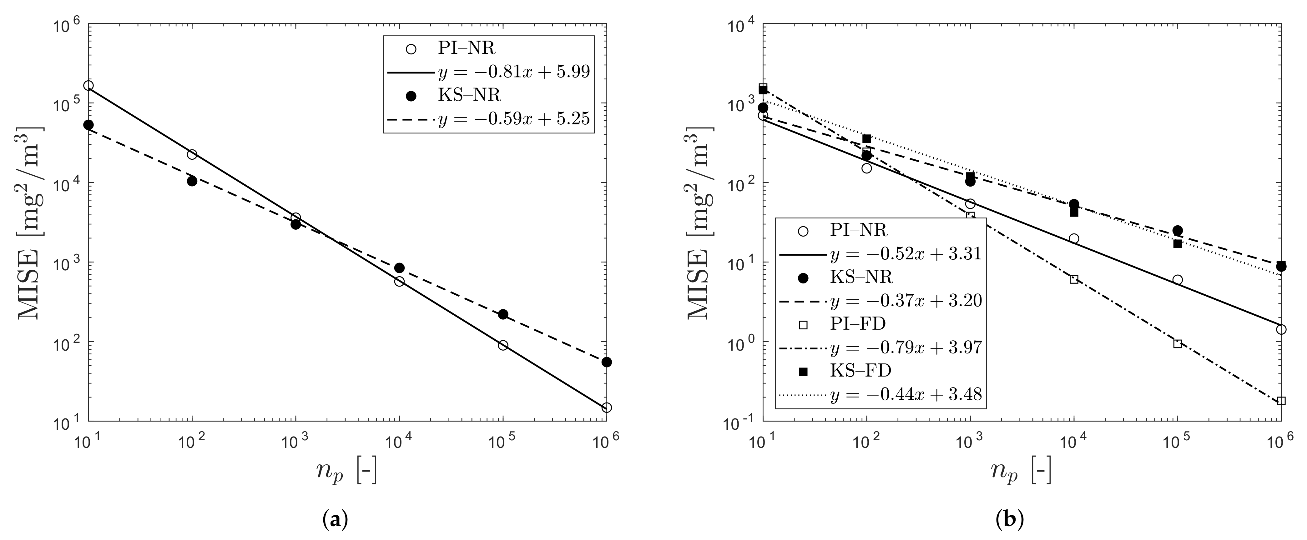
The MISE for the concentration field due to the instantaneous point release is calculated at two times corresponding with a mean drift of around 200and 1000 m , respectively. The results are presented in Table 2. The PI estimator is an unconditionally better estimator than the classical KS estimator if both its efficiency and convergence rate are higher. The convergence rate is theoretically expected to be higher, i.e., 4 / 5 vs. 4 / 7 . This is confirmed by the numerical simulations; for the shorter travel times, see the value of the β 0 parameter in Table 2 for NR. The abbreviation NR refers to the normal reference rule where the σ k in Equation (13) is estimated numerically from the solution. For the longer travel times, convergence is slower than what is theoretically expected.
In order to obtain a better insight into this behavior, the integrated Laplacian squared in Equation (8) also has been calculated numerically for the bandwidth of kernel K 1 in Equations (37) and (38). The objective is to investigate the influence of the boundary and therefore, only the bandwidth of kernel K 1 is modified since mainly the vertical concentration distribution is affected by the boundary. The crosswind-integrated concentration distribution for a unit source (p) has been estimated using a large number of particles ( n p = 10 8 p a r t i c l e s ) such that the effect of the chosen kernel and bandwidth (using the normal reference rule) can be neglected. A fourth-order central difference scheme has been used to approximate the second derivative of the distribution over height. Before the finite-difference scheme was applied, the concentration estimations were preprocessed with a linear noise filter to reduce oscillations in the estimated derivative. Finally, the integration was performed with the trapezoidal rule. The values of the estimated integrals are displayed in Table 3. Case I–HT for the 20 s travel time has been added as a benchmark, because the normal reference rule, Equation (13), is exact then. The finite-difference estimate (FD) and the analytical value (NR) coincide well for the latter case and this gives confidence that the procedure we are using is functioning properly. For cases II and III, there is a clear deviation between the FD and the NR estimate. Using the FD estimate in Equation (8) provides for a closer match with the theoretical convergence rate for both estimators, e.g., case III, see Figure 2b. Only for case I, the discrepancy becomes bigger then.
For two out of four cases, the PI estimator has, next to the higher convergence rate, also the highest efficiency (lower β 1 value). For the short travel times, these are cases I–HT and II. For the longer travel times, these are cases I–HT and I. For these cases, the MISE of the PI estimator is always lower than of KS. For the other cases, the MISE of the PI estimator is not unconditionally lower due to its higher β 1 value, but this is mostly not significant ( n p < 10 particles)—see Figure 2b as an example. Only for the short travel time in case III, see Figure 2a, a value of n p > 1000 particles is required for the PI estimator to have a lower MISE. Thus, one could state that the PI estimator has a nearly unconditionally lower MISE w.r.t. the KS estimator for the considered cases. Finally, the R 2 value in Table 2 confirms that the estimated MISEs are following a straight line w.r.t. n p , as is expected from the theory.

3.2. Demonstration on Project Prairie Grass

Project Prairie Grass [23,24] was a field program comprising 70 experiments conducted on a flat prairie in Nebraska in the summer of 1956. The program was conducted during July and August of 1956 with an equal number of experiments during the daytime and nighttime. Each time, the non-reactive, non-buoyant gas sulfur dioxide was released at a constant release rate. The time-averaged concentration was registered with 10-min samples downwind from a source release along five arcs and six towers. The arcs are located at 50, 100, 200, 400 and 800 m from the source and the towers are positioned along the arc at 100 m , spaced at 14 degrees intervals. The source was placed 0.46   m above the ground and can be treated as a point source. The concentration was measured at 1.5   m above the ground on the arcs and at nine different heights from 0.5   m to 17.5   m on the towers. In addition to the concentration measurements, the micro-meteorological conditions, including wind and temperature profiles, were registered as well along 16 m masts. From these profiles, Nieuwstadt [25] estimated the values of L and u * for various experiments taking the measurement error into account and assuming z 0 = 0.008 m . The obtained values of L and u * are listed for 60 experiments in [26], which have been adopted in the current work. In [25,26], the value κ = 0.35 was assumed from the 1968 Kansas experiments, whilst we assume κ = 0.387 [27]. Therefore, the values of u * in [26] need to be increased by 11 % ; the values of L are invariant w.r.t. this rescaling ([28], Equation (11.1), p. 214). The value of the mixing height for the unstable cases has been adopted from [29]. We estimated the mixing height for the stable cases as described in Appendix A.
We illustrate the model performance in the stable atmosphere for three experiments: 22, 29, 40. We selected experiments 15, 34 and 61 in the case of an unstable atmosphere. Experiment 22 and 34 have been selected for the high wind speed condition and the other experiments because of the greater amount of mesoscale variability. All the before-mentioned experiments also satisfy the requirement that the wind speed should be higher than 2 m s−1 at a height of 2 m , otherwise the measurement uncertainty on the meteorological quantities increases greatly ([23], Section 6.3, p. 207).
In order to assess the degree of convergence, the mean absolute relative error (MARE), the fractional bias (FB) and the fraction of predictions within the relative error of 5 % (FAC1.05) have been used, i.e.,
MARE = c ^ ( Δ t * , n p ) c ^ ( Δ t * / 2 , 50 n p ) 1 ¯ , FB = c ^ ( Δ t * / 2 , 50 n p ) ¯ c ^ ( Δ t * , n p ) ¯ 0.5 c ^ ( Δ t * / 2 , 50 n p ) ¯ + c ^ ( Δ t * , n p ) ¯ , FAC 1.05 = fraction of data that satisfy 0.95 c ^ ( Δ t * , n p ) c ^ ( Δ t * / 2 , 50 n p ) 1.05 ,
with c ^ the estimated concentration at the sampling stations, Δ t * = [ Δ t ] k / [ τ L ] k (specified in Section 2.5) and the overbar denotes the average over the data set. The error of 5 % in FAC1.05 has been chosen, because it represents the relative measurement error ([23], Section 5.6, p. 77). Note that the above measures compare two estimates of c ^ for which the total amount of particles differ with a factor of 100 ( Δ t * also controls the release time). The FB and FAC2 measures were introduced in [30] to compare model predictions with measurements, but here it is used to assess the different levels of convergence as mentioned before.
The results of the convergence study for a stable atmosphere can be found in Table 4. All predictions lower than the detection limit of 0.1  mg m−3 ([23], Section 5.6, p. 77) are treated as noise and they have been excluded. All statistics indicate that the PI estimator obtains a higher degree of convergence than the KS estimator does in a stable atmosphere. In this case, the PI estimator has a MARE that is a factor of five smaller, a FB that is a factor of four smaller and a FAC1.05 that is a factor of 2.6 higher for n p = 1000 particles per release time and Δ t * = 0.05 . These parameter settings correspond with a release of around 7.6 million particles in total.
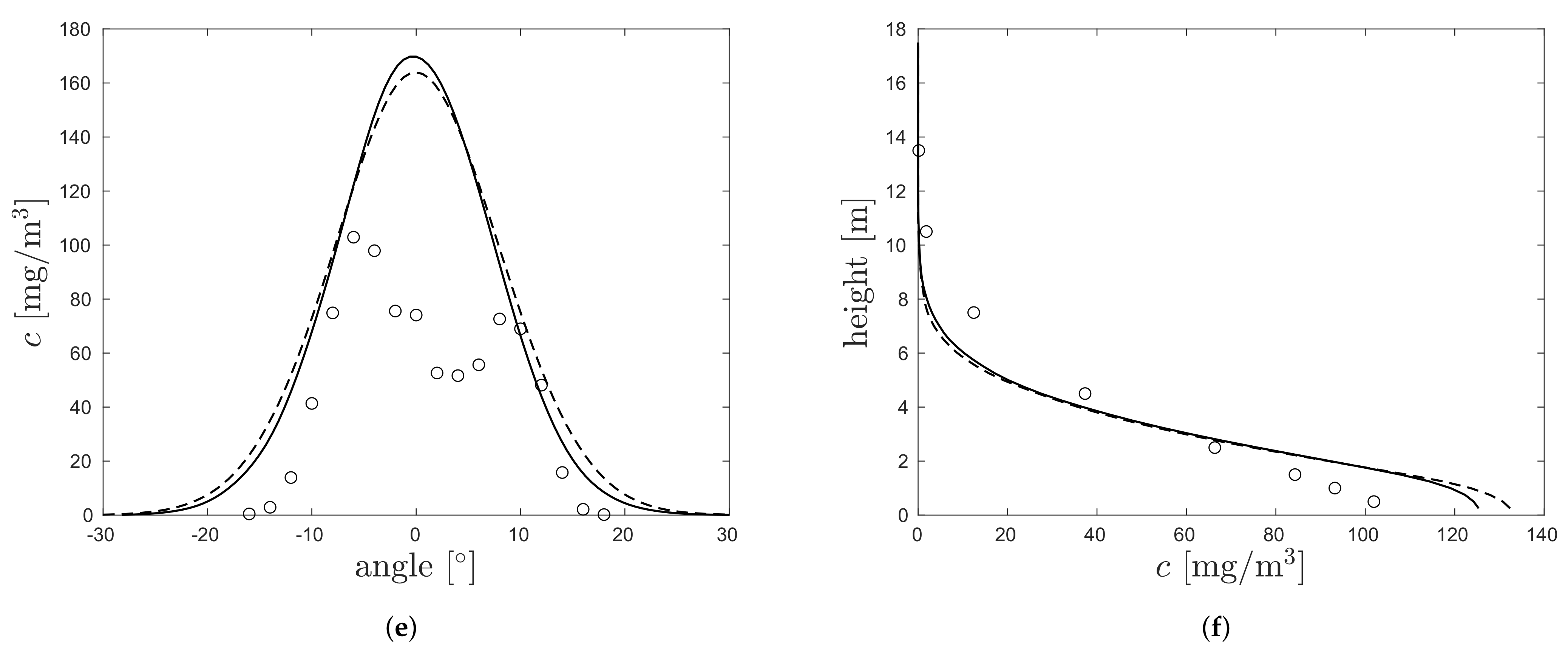
In Figure 3, crosswind and vertical concentration profiles from the PI and KS estimator are shown for the 100 m -arc. Recall from Section 3.1 that KS has a uniform slower convergence in n p in a stable atmosphere. As a result, we observe that it predicts the maximum value of the crosswind profiles 6.6 % lower on average than the PI estimator does at the arcs for the chosen values of n p and Δ t * , e.g., see Figure 3 a,c,e. Since this deviation exceeds the measurement error, it cannot be neglected. The lower peak value predicted by KS results in a broader distribution w.r.t. PI. This is also visible as higher-predicted concentrations near the ground in the vertical profiles (not the centerline profile), see Figure 3 b,d,f.
For the sake of completeness, the predictive capabilities of the PI estimator are briefly discussed. The predictions for experiment 22 suffer from a bias in wind direction. Nonetheless, the magnitude of the peak value is well predicted at the 100 m -arc (Figure 3a). At the 50 m and 200 m -arc, its magnitude is under- and overestimated by 16 % , respectively. In experiment 29, the width of the concentration distribution is underestimated. The discrepancy is mainly present in the left half of the distribution, see Figure 3c. The magnitude of the maximum values tend to be overestimated at all the arcs but always less than 16 % . In experiment 40, the width of the distribution tends to be slightly overestimated at all the arcs, e.g., see Figure 3e. The maximum values are approximately overestimated with 60 % at the 50 , 100 and 200 m -arc. Generally, one can say that the height-dependent profiles are best predicted at the towers closest to the wind direction. These are the tower measurements displayed in Figure 3. In experiment 40, the wind direction was positioned exactly midway between two towers. Figure 3f only shows one of them, but a similar result has been obtained for the other tower with an overestimation near the ground surface. The vertical extent of the plume is reasonably predicted for experiment 22 (Figure 3b).
Table 4 shows that it is harder to obtain good convergence in case of an unstable atmosphere. Again, all predictions lower than the detection limit of 0.1  mg m−3 ([23], Section 5.6, p. 77) have been excluded. The statistics indicate as well that the PI estimator obtains a higher degree of convergence for an unstable atmosphere than the KS estimator does. The PI estimator has a MARE that is a factor of 2.5 smaller, a similar FB and a FAC1.05 that is a factor of 2 higher for n p = 1000 particles per release time and Δ t * = 0.01 . These parameter settings correspond with a release of around 15 million particles in total.
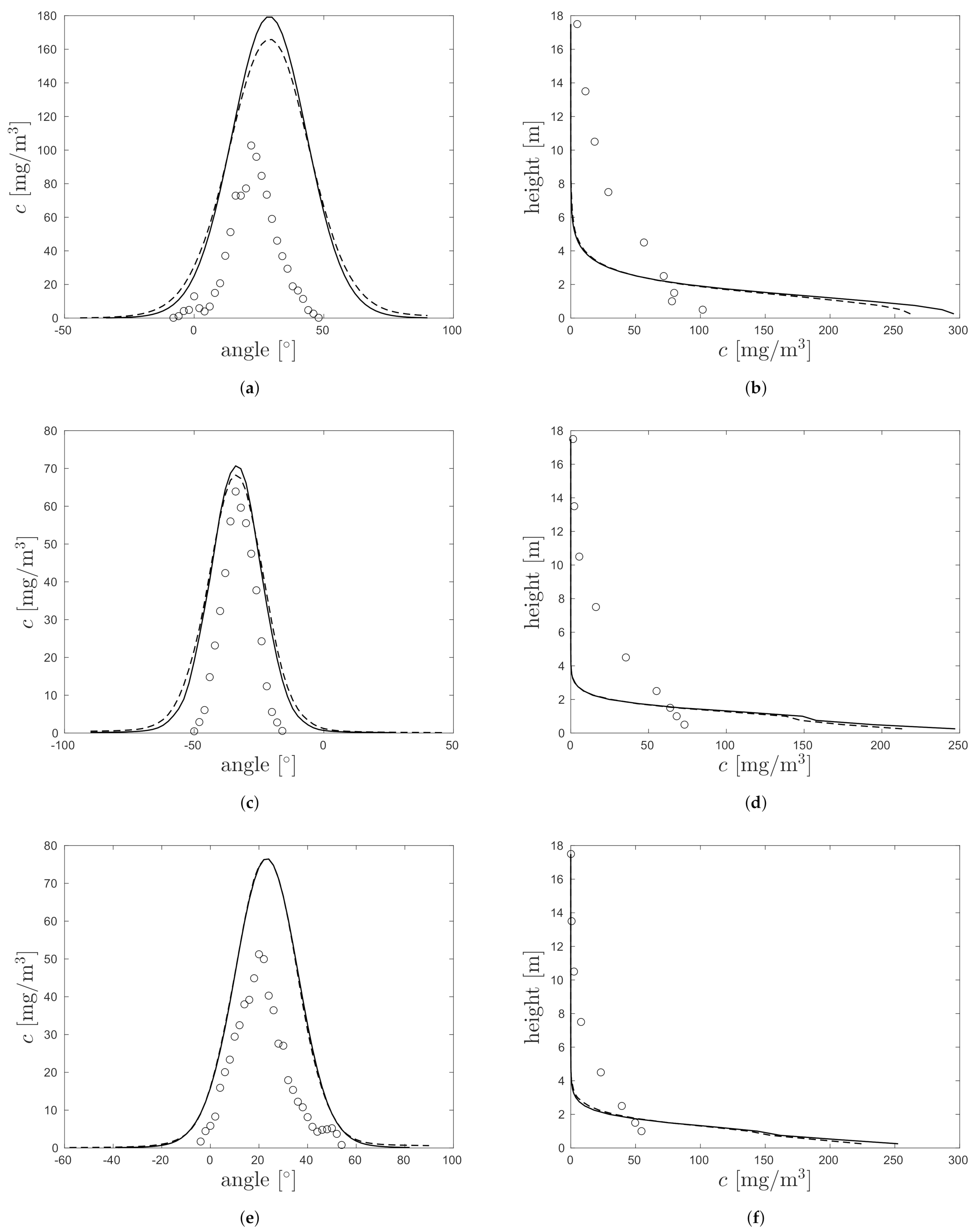
In Figure 4, crosswind and vertical concentration profiles by the PI and KS estimator are shown for the 100 m -arc. Just as with the stable atmosphere, the predicted profiles do not coincide completely due to a different convergence behavior. Recall from Section 3.1 that the PI estimator convergences faster in an unstable atmosphere if the chosen number of particles is sufficiently high. Table 4 confirms that this is the case. We observe that the PI estimator predicts the maximum value of the crosswind profiles 22 % higher on average than the KS estimator does at the arcs for the chosen values of n p and Δ t * , e.g., see Figure 4a,c,e. This deviation also exceeds the measurement error and therefore, it cannot be neglected.
Finally, the predictive capabilities of the PI estimator are briefly discussed. All three experiments show a similar pattern: at the 50 and 100 m -arc the concentrations are under- and overestimated, respectively, with an average deviation of 45 % . From the 200 m -arc, the overestimation is more than a factor of two. In general, there seems to be a tendency to overestimate the width of the crosswind distribution in an unstable atmosphere, as can be seen from Figure 4a,c,e. As before, the tower measurements in Figure 4 were taken from the towers positioned closest to the wind direction. For each experiment, the vertical extent of the plume is underestimated with an overestimation near the ground surface as a consequence (Figure 4b,d,f).

4. Discussion

In Table 2, one observes that the convergence rates for a longer travel time deviate more from the theoretical rate than for a short travel time. Two possible hypotheses can be formulated: (1) the convergence is slowed down due to a non-zero vertical gradient of the underlying density at the boundary, as discussed in [31]; (2) the concentration field deviates more from a Gaussian distribution for longer travel times, consequently the normal reference rule used to evaluate Equation (8) is no longer appropriate. What also contributes to the non-validity of this rule for the longer travel times is that it does not take the ground surface into account. It can be observed that evaluating instead the integral of the Laplacian squared for the crosswind-integrated concentration distribution (see Table 3) numerically improves the convergence rates, except for case I. Recall that the KS estimator also uses the normal reference rule to estimate the concentration in the horizontal plane. This may also contribute to the discrepancy that is still present in the convergence rate of the KS–FD estimator, for example, in case III. Small deviations from the theoretical convergence rate that are present as well in the PI–FD estimator are most likely due to numerical errors in the estimation of the second derivative and the integration used for the MISE. Due to the better correspondence with the theory by avoiding the normal reference rule in the vertical direction, the second hypothesis is plausible. This suggests that using more sophisticated bandwidth selection methods than the normal reference rule will improve the convergence rates. It was found in [32] that sophisticated bandwidth selection methods do not have a superior performance for larger distances downwind of 1 – 50 k m and higher effective release heights of 100 – 300 m . It seems to us rather unlikely that the first hypothesis can explain the discrepancy in the neutral atmosphere, since perfect reflection imposes a zero gradient at the boundary. This cannot be seen on Figure 1c because the resolution near the ground surface is not high enough to resolve this gradient properly. It is striking to conclude that up to 35 % of the convergence speed can be lost with the normal reference rule. This can increase the number of particles required to gain one digit of accuracy with a factor of five or nine, depending on the estimator. Of course, such issues have already been addressed in the literature and numerically more intensive methods have been developed to select the optimal bandwidth. An example is the plug-in bandwidth selector, which is widely recommended ([8], Section 2.4, p. 26). This selector also uses the asymptotic approximation in Equation (8), but one should realize that this comes with the cost of evaluating ( 1 ) n p ( n p + 1 ) / 2 kernels more per instantaneous release where is the selected stage. A plug-in bandwidth selector that is completely independent of a normal reference rule is proposed by [11] for their 1D diffusion kernel, which is also a type of kernel smoother. An alternative to the plug-in selector is provided by the smoothed cross validation bandwidth selector, which does not rely on the asymptotic approximation in Equation (8). Despite the added computational complexity, it is not clear whether this selector performs better than the plug-in selector. More information and other bandwidth selection methods that could be used can be found in ([8], Chapter 3, pp. 43–66).
Whether the PI or KS estimator is better does not only depend on the convergence rate but also on the efficiency of the estimator (parameter β 1 in Table 2). As already remarked in Section 3.1, the proposed PI estimator has a comparable efficiency as the 3D Epanechnikov estimator, used in the KS estimator. Consequently, it can be considered as the better estimator due to the predominantly higher convergence rate. The main advantage of the proposed PI estimator is that it allows for faster dispersion simulations over homogeneous terrain since it reduces the sampling cost for the particles and it converges faster. Profiling the code of the KS estimator during the simulation of experiments 22, 40, 15 and 34 showed that the calls to the random number generator represent up to 35 % of the total runtime. Thus, this cost is definitely not negligible. The PI estimator reduces this cost with a factor of three for a given number of particles. The cost reduction for a given accuracy can be expected to be much higher due to the improved convergence rate. Table 4 supports this argument. Note that this improved convergence has been obtained by exploiting the assumptions of horizontally homogeneous meteorological conditions. On top of this, additional mathematical techniques can be applied for further improvements. As an example, it might be interesting to choose the kernel smoother in Equation (24) as the geometric extrapolated bias-reduced kernel of [9] such that the convergence rate to estimate the 3D concentration can even be further improved up to 12 / 13 . Because of the improved accuracy, the PI estimator would be an excellent validation tool for Langevin models that can take more complex terrain configurations into account. After all, if such models are applied to horizontally homogeneous terrain, then their results should coincide with those of the PI estimator over such terrain in the near-field range.
Table 4 makes clear that obtaining the same degree of convergence for the KS as for the PI estimator requires some additional resources. Note that in order to make a qualitative comparison with measurements, the convergence error should preferably be below the relative measurement error of 5 % . We found that convergence is easier obtained in the near-field range with the parameterization for the stable atmosphere than for the unstable one. In the latter, the larger Lagrangian time scales in the horizontal directions lead to time steps, which cannot be made sufficiently small as required for numerical convergence due to the physical restriction on the time step, see Section 2.5. Thus, the physical and numerical requirements are conflicting. It is not clear to us how this issue can be overcome.

5. Conclusions

A new kernel density estimator derived from the Langevin equation has been presented for dispersion assuming local Gaussian turbulence and horizontally homogeneous meteorological conditions. The latter assumption is often relevant for near-field range dispersion studies. The new estimator has the special property that only the vertical particle positions need to be calculated numerically. Consequently, the convergence rate of a 1D kernel smoother is inherited.
The convergence study confirms the higher convergence rate. We found that for longer travel times, the numerical convergence rate deviates from the theoretical one for both estimators. We argued that this may be due to the use of the normal reference rule in the bandwidth calculation. The efficiency of the newly proposed estimator has been found to be comparable with the one of the optimal 3D Epanechnikov kernel, except possibly in an unstable atmosphere. For this type of stratification, the efficiency of the proposed estimator may be lower. Consequently, it has been found that the convergence in MISE sense is only conditionally faster, depending on the released number of particles. For a stable or neutral atmosphere, the convergence of the proposed estimator has been found to be unconditionally faster w.r.t. the 3D kernel smoother. In the Project Prairie Grass experiment, the improved convergence allows obtaining the convergence error for at least twice as many predictions below the relative measurement error than with the 3D kernel smoother.
It still needs to be verified whether the theoretical convergence rate can be more closely resembled if a more sophisticated bandwidth selection method is used, such as the plug-in bandwidth selector. It may also be interesting to conduct a sensitivity study of the model input parameters in order to quantify what part of the observed discrepancies between the model predictions and the measurements is due to the measurement error.

Author Contributions

Conceptualization, G.B. and J.M.; methodology, G.B. and J.M.; software, G.B.; validation, G.B.; formal analysis, G.B.; investigation, G.B.; resources, J.M.; data curation, G.B.; writing—original draft preparation, G.B.; writing—review and editing, J.M.; visualization, G.B.; supervision, J.M.; project administration, G.B. All authors have read and agreed to the published version of the manuscript.

Funding

This research received no external funding.

Data Availability Statement

No new data were created or analyzed in this study. Data sharing is not applicable to this article.

Acknowledgments

The authors would like to thank Pieter De Meutter and Tim Vidmar for their constructive comments on the first draft of this paper as well as the anonymous reviewers for their valuable remarks.

Conflicts of Interest

The authors declare no conflict of interest.

Appendix A. Atmospheric Parameterization

The form of the input functions α , a and b in Equation (3) is chosen such that particle dispersion in a vertically inhomogeneous flow is adequately parameterized. It is sufficient to demand that the model satisfies the well-mixed condition, i.e., if the particles of a tracer are initially well mixed, then they should remain so. The following parameterization is adopted such that this criterion is satisfied [33] ( k = 1 , 2 , 3 )
α k ( z ) = 1 [ τ L ( z ) ] k , a z , w = 1 2 w 2 σ w 2 ( z ) + 1 d σ w 2 d z ( z ) , b k ( z ) = [ σ u ( z ) ] k 2 [ τ L ( z ) ] k ,
with τ L R 3 the Lagrangian time scale vector ( s ) and σ u = ( σ u , σ v , σ w ) R 3 the variance vector ( m / s ) of the particle velocity. Here, the operator [ · ] k returns the k-th component of the input vector.
The meteorological quantities u , τ L and σ u are parameterized to represent the different atmospheric conditions. In the current work, a conventional open-field model based on Monin–Obukhov similarity theory (MOST) is used. The Eulerian wind profile according to MOST is given by (e.g., [34], Section 9.7.5, p. 385)
u = u ¯ e ^ ϕ , u ¯ ( z ; u * , L ) = u * κ ln z z 0 Ψ M ( z / L ) + Ψ M ( z 0 / L ) ,
with e ^ ϕ the unit vector aligned with the wind direction ϕ , u * the friction velocity ( m / s ), κ = 0.387 the von Kármán constant (-) [27], z 0 the roughness length ( m ), L the Monin–Obukhov length ( m ) and Ψ M the integrated stability kernel, i.e.,
Ψ M ( ξ ) = 4.7 ξ , ξ > 0 , Ψ M ( ξ ) = ln 1 + x 2 2 1 + x 2 2 2 arctan x + π 2 , x = ( 1 15 ξ ) 1 / 4 , ξ < 0 .
In the surface layer, the variance of the horizontal wind components can be assumed to be independent of height for every stratification regime. The variance of the vertical wind component is also height independent, except in an unstable atmosphere according to local free convection similarity theory. These variances are parameterized as follows
σ u 2 = 6.3 u * 2 , σ v 2 = 4.1 u * 2 , σ w 2 = 1.7 u * 2 , | L | > 200 m ,
σ u 2 = 8.5 u * 2 σ v 2 , σ v = 1.7 u * , σ w 2 = 2.5 u * 2 , 0 < L < 200 m ,
σ u = σ v = 0.6 u * 3 κ L h i 1 / 3 , σ w ( z ) = 1.4 u * 3 κ L z 1 / 3 , 200 m < L < 0 .
The relationship σ v = 1.7 u * for a stable stratification has been adopted from [35] for short grassland. The unstable parameterization can be found in ([28], Section 11.5, p. 237, Equation (11.1), p. 214, Equation (9.41), p. 183, Equation (9.43), p. 184). The rest has been adopted from [34].
The Lagrangian time scale τ L is considered to be a three-dimensional vector; a parameterization for each component can be found in [36], i.e.,
τ L 1 = [ τ L ] 2 = [ τ L ] 3 = 0.5 z / σ w 1 + 15 f C z / u * , | L | 200 m ,
τ L = 0.15 σ u h i z , 0.07 σ v h i z , 0.1 σ w h i 0.2 z 0.8 , 0 m < L < 200 m ,
τ L ] 1 = [ τ L ] 2 = 0.15 h i σ u , 200 m < L < 0 m ,
τ L ] 3 = 0.1 z σ w [ 0.55 + 0.38 ( z z 0 ) / L ] , 200 m < L < 0 m a n d z < 0.1 h i a n d z z 0 < L ,
τ L ] 3 = 0.59 z / σ w , 200 m < L < 0 m a n d z < 0.1 h i a n d z z 0 > L ,
τ L ] 3 = 0.15 h i σ w 1 exp 5 z h i , 200 m < L < 0 m a n d z > 0.1 h i .
The expression for τ L in stable and unstable conditions requires the height of the mixed layer, h i , as an input. Preferably, this quantity is measured, but if this is not the case, then it needs to be parameterized. In case of a stable atmosphere, the height is estimated as h i = 0.4 u * L / f C ( 0 m < L < 200 m ) [37] with f C the Coriolis parameter. In case of an unstable atmosphere, we assume that h i is known (see Section 3.2). According to the above formulas, note that [ τ L ] 1 = [ τ L ] 2 is immediately satisfied for a neutral and unstable stratification throughout the entire boundary layer. According to (A3), σ u = 1.4 σ v and [ τ L ] 1 σ v 0.1 h i z . For implementation technical reasons, we assume that [ τ L ] 1 = [ τ L ] 2 0.085 h i z / σ v for 0 m < L < 200 m , which is only a minor modification.
One should realize that Equations (A2)–(A4) only represent the turbulence velocity variance. These variances do not necessarily explain all the measured variability ( σ tot ), because there might be a contribution from mesoscale motions. Vickers and Mahrt [35] discuss this phenomenon in particular for the stable boundary layer. They also argue that turbulence motions have a different effect on dispersion than mesoscale motions do. Therefore, one should distinguish between both types of variability. The turbulence component will be treated as internal variability generated by the model and the mesoscale component will be added as external variability ( σ e ). There holds [35]
σ tot 2 = σ e 2 + σ v 2 .
Denote σ ϕ ( ) the wind direction standard deviation and presume that σ ϕ σ tot / u ¯ ( 180 / π ) is sufficiently small, then by Equation (A11) the mesoscale component of the standard deviation σ ϕ , e ( ) satisfies
σ ϕ , e 2 σ ϕ 2 T I 2 180 2 π 2
with T I = σ v / u ¯ [−] the lateral turbulence intensity. If (A12) is negative, then the distribution of Φ is assumed to be degenerated in ϕ ¯ , the time-averaged wind direction. Otherwise, the wind direction is modeled as
Φ = ϕ ¯ + Φ , Φ N ( 0 , σ ϕ , e 2 ) .
Section 2.5 provides more details about the application of Equation (A13) in the particle model. Vervecken et al. [38] used a similar approach in the framework of the advection-diffusion equation.
Finally, we remark that the above relations relate to classical Monin–Obukhov theory for flat open terrain. Other parameterizations of homogeneous terrain that can be relevant may, e.g., be the forest. See, for instance, [39].

Appendix B. The Wiener Measure Applied to the Langevin Equation

In Equation (14), we integrate over the paths of the stochastic process ( Z s ) s > t . The aim of this section is to properly define such an integral if ( Z s ) s > t satisfies the Langevin equation. Denote the space of all paths [ t , t ] R by X . Consider a function f : X R whose image depends on the entire path { Z s , t s t } . Its functional average can be evaluated if one can properly integrate over all the possible paths. In order to do this, an appropriate measure d W z ( s ) should be formulated such that
f ( { z s , t s t } ) d W z ( s ) , d W z ( s ) = p ( { z s , t s t } ) d z ( s ) ,
is well defined. In the above formula, p ( { Z s , t s t } ) represents the time-dependent distribution of the paths and d z ( s ) denotes the integration over the paths. Determining the measure d W z ( s ) comes down to interpreting the path distribution meaningfully.
We follow the approach of [12]. Discretize the paths: let the Eulerian variable z k denote the value of a path at time t k such that t k 1 < t k < t k + 1 ( k = 1 , , n 1 ) with t = t 0 and t n = t , then
f ( { z s , t s t } ) d W z ( s ) = lim n max k Δ t k 0 0 + 0 + f ( z 0 , , z n ) p ( z 0 , , z n ) d z 0 d z n
with
f ( { z s , t s t } ) = lim n max k Δ t k 0 f ( z 0 , , z n )
and p ( z 1 , , z n ) the common distribution of ( Z 0 , , Z n ) . If ( Z s ) s > t is a Wiener process, then d W z ( s ) coincides with the classical Wiener measure [12], which measures the probability that a path is realized. The Wiener measure is well defined as a probability measure, because the Chapman–Kolmogorov property is satisfied for the Wiener process (and Itô processes in general), see ([40], Section 1.1.3, p. 36), due to its Markov property, i.e., its transition probability density function satisfies the relationship
p ( t , z | t , z 0 ) = 0 + p ( t , z | t , z ) p ( t , z | t , z 0 ) d z .
Now, the functional average can be meaningfully defined as
E f ( { Z s , t s t } ) = f ( { Z s , t s t } ) d W z ( s ) = lim n max k Δ t k 0 0 + 0 + f ( z 0 , , z n ) p ( z 0 ) k = 1 n p ( z k | z k 1 ) d z 0 d z n .
In the case of the Langevin process, the evolution of the state of ( Z s ) s > t can be considered as a Markov process in the position-velocity phase space, as was done previously by [41]. Consequently, a similar relationship as in Equation (A16) holds, which is also integrated over the speed ( Z ˙ s ) s > t . There follows,
E f ( { Z s , t s t } ) = lim n max k Δ t k 0 0 + + 0 + + 0 + f ( z 0 , , z n ) p ( z 0 , z ˙ 0 ) k = 1 n 1 p ( z k , z ˙ k | z k 1 , z ˙ k 1 ) p ( z n | z n 1 , z ˙ n 1 ) d z 0 d z ˙ 0 d z n 1 d z ˙ n 1 d z n
with f ( z 0 , , z n ) as in Equation (A15). Note that p ( z 0 , , z n ) is considered as the marginal distribution of p ( z 0 , , z n , z ˙ 0 , , z ˙ n ) . The principles set out in this section apply to Equations (14), (17) and (23).

Appendix C. Derivation of the Recursion Formula for D nk,k

Consider times t < t 1 < < t n and discretize the functions α k and b k such that their values are constant over the intervals [ t m , t m + 1 ] ( m = 0 , , n 1 ) , denoted by α k m and b k m , then
D k , k n = t t n 1 s t n e s q α k ( z l ) d l d q b k 2 ( z s ) 2 d s + b k n 1 2 t n 1 t n s t n e s q α k ( z l ) d l d q 2 d s .
In the second term on the left-hand side, one can write s q α k ( z l ) d l = α k n 1 ( q s ) , consequently
b k n 1 2 t n 1 t n s t n e α k n 1 ( q s ) d q 2 d s = ( b k n 1 ) 2 2 ( α k n 1 ) 3 e α k n 1 Δ t n 2 2 + ( b k n 1 ) 2 ( α k n 1 ) 2 Δ t n 1 2 α k n 1 .
By splitting the integral inside the square in the first term on the left-hand side of Equation (A17) over the intervals [ s , t n 1 ] and [ t n 1 , t n ] , one obtains
D k , k n 1 + t t n 1 t n 1 t n e s q α k ( z l ) d l d q b k 2 ( z s ) 2 d s + 2 t t n 1 b k 2 ( z s ) s t n 1 e s q α k ( z l ) d l d q t n 1 t n e s q α k ( z l ) d l d q d s .
The second term in (A18) can be written as
t t n 1 b k 2 ( z s ) e 2 s t n 1 α k ( z l ) d l d s t n 1 t n e s q α k ( z l ) d l d q 2 = 1 ( α k n 1 ) 2 e α k n 1 Δ t n 1 2 D ˜ k n 1 ,
D ˜ k n 1 : = t t n 1 b k 2 ( z s ) e 2 s t n 1 α k ( z l ) d l d s .
The third term in (A18) equals
2 t n 1 t n e α k n 1 ( q t n 1 ) d q t t n 1 b k 2 ( z s ) s t n 1 e s q α k ( z l ) d l d q e s t n 1 α k ( z l ) d l d s = 2 α k n 1 e α k n 1 Δ t n 1 D ^ k n 1 , D ^ k n 1 : = t t n 1 b k 2 ( z s ) s t n 1 e s q α k ( z l ) d l d q e s t n 1 α k ( z l ) d l d s .
The expression for D ^ k n 1 can be rewritten as
D ^ k n 1 = e α k n 2 Δ t n 1 D ^ k n 2 + b k n 2 2 t n 2 t n 1 s t n 1 e s q α k ( z l ) d l d q e s t n 1 α k ( z l ) d l d s + t t n 1 b k 2 ( z s ) t n 2 t n 1 e s q α k ( z l ) d l d q e s t n 1 α k ( z l ) d l d s .
The second term in the sum in (A22) equals
b k n 2 2 2 ( α k n 2 ) 2 1 e α k n 2 Δ t n 1 2 .
The third term in the sum in (A22) equals
t n 2 t n 1 e α k n 1 Δ t n 1 d q i = 0 n 3 t i t i + 1 b k i 2 e 2 s t i + 1 α k ( z l ) d l d s e 2 t i + 1 t n 1 α k ( z l ) d l = 1 α k n 2 1 e α k n 2 Δ t n 1 D ¯ k n 1 , D ¯ k n 1 : = i = 0 n 3 b k i 2 2 α k i 1 e 2 α k i Δ t i + 1 e 2 t i + 1 t n 1 α k ( z l ) d l .
It can be easily verified that the recursive scheme for D ¯ k n 1 is given by (36).

References

  1. Izenman, A.J. Recent developments in nonparametric density estimation. J. Am. Stat. Assoc. 1991, 86, 205–224. [Google Scholar] [CrossRef]
  2. Rosenblatt, M. Remarks on some nonparametric estimates. Ann. Math. Stat. 1956, 27, 832–837. [Google Scholar] [CrossRef]
  3. Parzen, E. On estimation of a probability density function and mode. Ann. Math. Stat. 1962, 33, 1065–1076. [Google Scholar] [CrossRef]
  4. Lorimer, G.S. The kernel method for air quality modelling–I. mathematical foundation. Atmos. Environ. 1986, 20, 1447–1452. [Google Scholar] [CrossRef]
  5. Fasoli, B.; Lin, J.C.; Bowling, D.R.; Mitchell, L.; Mendoza, D. Simulating atmospheric tracer concentrations for spatially distributed receptors: Updates to the Stochastic Time-Inverted Lagrangian Transport model’s R interface (STILT-R version 2). Geosci. Model Dev. 2018, 11, 2813–2824. [Google Scholar] [CrossRef] [Green Version]
  6. Björnham, O.; Brännström, N.; Grahn, H.; Lindgren, P.; von Schoenberg, P. Post-Processing of Results from a Particle Dispersion Model by Employing Kernel Density Estimation; Technical Report FOI-R–4135–SE; FOI: Stockholm, Sweden, 2015. [Google Scholar]
  7. Stohl, A.; Forster, C.; Frank, A.; Seibert, P.; Wotawa, G. The Lagrangian particle dispersion model FLEXPART version 6.2. Atmos. Chem. Phys. 2005, 5, 2461–2474. [Google Scholar] [CrossRef] [Green Version]
  8. Chacón, J.E.; Duong, T. Multivariate Kernel Smoothing and Its Applications, 1st ed.; Number 160 in Monographs on Statistics and Applied Probability; CRC Press: Boca Raton, FL, USA, 2018; p. 248. [Google Scholar]
  9. Xie, X.R.; Wu, J.J. Some Improvement on Convergence Rates of Kernel Density Estimator. Appl. Math. 2014, 5, 1684–1696. [Google Scholar] [CrossRef] [Green Version]
  10. Crawford, A. The use of Gaussian mixture models with atmospheric Lagrangian particle dispersion models for density estimation and feature identification. Atmosphere 2020, 11, 1369. [Google Scholar] [CrossRef]
  11. Botev, Z.I.; Grotowski, J.F.; Kroese, D.P. Kernel density estimation via diffusion. Ann. Stat. 2010, 38, 2916–2957. [Google Scholar] [CrossRef] [Green Version]
  12. Wiener, N. The average of an analytic functional. Proc. Natl. Acad. Sci. USA 1921, 7, 253–260. [Google Scholar] [CrossRef] [PubMed] [Green Version]
  13. Alvarez, A.; Pennel, R.; Garau, B.; Tintore, J. A Fourier-transform path integral formalism to compute dispersion probability distributions in variable ocean environments. Geophys. Res. Lett. 2007, 34. [Google Scholar] [CrossRef] [Green Version]
  14. Hurley, P. PARTPUFF—A Lagrangian Particle-Puff Approach for Plume Dispersion Modeling Applications. J. Appl. Meteorol. Climatol. 1994, 33, 285–294. [Google Scholar] [CrossRef] [Green Version]
  15. Lamb, R.G. Diffusion in the convective boundary layer. In Atmospheric Turbulence and Air Pollution Modelling; Springer: Berlin/Heidelberg, Germany, 1984; Volume 1, pp. 159–229. [Google Scholar]
  16. Kloeden, P.E.; Platen, E. Numerical Solution of Stochastic Differential Equations, 2nd ed.; Stochastic Modelling and Applied Probability; Springer-Verlag: Berlin/Heidelberg, Germany, 1992; Volume 23. [Google Scholar]
  17. Thomson, D.J.; Wilson, J.D. Lagrangian Modeling of the Atmosphere; Geophysical Monograph Series; Chapter History of Lagrangian Stochastic Models for Turbulent Dispersion; American Geophysical Union: Washington, DC, USA, 2012; Volume 200, pp. 19–36. [Google Scholar]
  18. Müller, H.G. Nonparametric Regression Analysis of Longitudinal Data, 1st ed.; Lecture Notes in Statistics; Springer: New York, NY, USA, 1988; Volume 46, pp. XIV, 369. [Google Scholar]
  19. Silverman, B.W. Density Estimation for Statistics and Data Analysis; Chapman and Hall/CRC: London, UK, 1986; Monographs on Statistics and Applied Probability. [Google Scholar]
  20. Paley, R.E.A.C.; Wiener, N.; Zygmund, A. Notes on random functions. Math. Z. 1933, 37, 647–668. [Google Scholar] [CrossRef]
  21. Nasstrom, J.S.; Ermak, D.L. A homogeneous Langevin equation model, part II: Simulation of dispersion in the convective boundary layer. Bound. Layer Meteorol. 1999, 92, 371–405. [Google Scholar] [CrossRef]
  22. Legg, B.; Raupach, M. Markov-chain simulation of particle dispersion in inhomogeneous flows: The mean drift velocity induced by a gradient in Eulerian velocity variance. Bound. Layer Meteorol. 1982, 24, 3–13. [Google Scholar] [CrossRef]
  23. Barad, M.L. Project Prairie Grass, a Field Program in Diffusion; Technical Report 59; Air Force Cambridge Research Center: Bedford, MA, USA, 1958; Volume I & II. [Google Scholar]
  24. Haugen, D.A. Project Prairie Grass, a Field Program in Diffusion; Technical Report 59; Air Force Cambridge Research Center: Bedford, MA, USA, 1959; Volume III. [Google Scholar]
  25. Nieuwstadt, F. The computation of the friction velocity u* and the temperature scale T* from temperature and wind velocity profiles by least-square methods. Bound. Layer Meteorol. 1978, 14, 235–246. [Google Scholar] [CrossRef]
  26. Van Ulden, A.P. Simple estimates for vertical diffusion from sources near the ground. Atmos. Environ. 1978, 12, 2125–2129. [Google Scholar] [CrossRef]
  27. Andreas, E.L.; Claffey, K.J.; Jordan, R.E.; Fairall, C.W.; Guest, P.S.; Persson, P.O.G.; Grachev, A.A. Evaluations of the von Kármán constant in the atmospheric surface layer. J. Fluid Mech. 2006, 559, 117–149. [Google Scholar] [CrossRef] [Green Version]
  28. Arya, S.P. Introduction to Micrometeorology, 2nd ed.; International Geophysics Series; Academic Press: Cambridge, MA, USA, 2001; Volume 79. [Google Scholar]
  29. Briggs, G.A.; McDonald, K.R. Prairie Grass revisited: Optimum indicators of vertical spread. In Proceedings of the 9th NATO-CCMS International Technical Symposium on Air Pollution Modeling and its Application, Toronto, ON, Canada, 28–31 August 1978; pp. 209–220. [Google Scholar]
  30. Chang, J.C.; Hanna, S.R. Air quality model performance evaluation. Meteorol. Atmos. Phys. 2004, 87, 167–196. [Google Scholar] [CrossRef]
  31. Marron, J.S.; Ruppert, D. Transformations to reduce boundary bias in kernel density estimation. J. R. Stat. Soc. B 1994, 56, 653–671. [Google Scholar] [CrossRef]
  32. Vitali, L.; Monforti, F.; Bellasio, R.; Bianconi, R.; Sachero, V.; Mosca, S.; Zanini, G. Validation of a Lagrangian dispersion model implementing different kernel methods for density reconstruction. Atmos. Environ. 2006, 40, 8020–8033. [Google Scholar] [CrossRef]
  33. Thomson, D.J. Criteria for the selection of stochastic models of particle trajectories in turbulent flows. J. Fluid Mech. 1987, 180, 529–556. [Google Scholar] [CrossRef]
  34. Stull, R.B. Chapter 9: Similarity Theory. In An Introduction to Boundary Layer Meteorology (Atmospheric Sciences Library); Kluwer Academics Publishers: Dordrecht, The Netherlands, 1988; Volume 13, pp. 347–404. [Google Scholar]
  35. Vickers, D.; Mahrt, L. Observations of the cross-wind velocity variance in the stable boundary layer. Environ. Fluid Mech. 2007, 7, 55–71. [Google Scholar] [CrossRef]
  36. Hanna, S.R. Applications in air pollution modeling. In Atmospheric Turbulence and Air Pollution Modelling; Springer: Berlin/Heidelberg, Germany, 1984; Volume 1, pp. 275–310. [Google Scholar]
  37. Caughey, S.J. Observed characteristics of the atmospheric boundary layer. In Atmospheric Turbulence and Air Pollution Modelling; Springer: Berlin/Heidelberg, Germany, 1984; pp. 107–158. [Google Scholar]
  38. Vervecken, L.; Camps, J.; Meyers, J. Accounting for wind-direction fluctuations in Reynolds-averaged simulation of near-range atmospheric dispersion. Atmos. Environ. 2013, 72, 142–150. [Google Scholar] [CrossRef] [Green Version]
  39. Bijloos, G.; Camps, J.; Tubex, L.; Meyers, J. Parametrization of homogeneous forested areas and effect on simulated dose rates near a nuclear research reactor. J. Environ. Radioact. 2020, 225, 106445. [Google Scholar] [CrossRef] [PubMed]
  40. Chaichian, M.; Demichev, A. Path Integrals in Physics; Stochastic Processes and Quantum Mechanics; CRC Press: Boca Raton, FL, USA, 2001; Volume 1, p. 336. [Google Scholar]
  41. Obukhov, A.M. Description of turbulence in terms of Lagrangian variables. Adv. Geophys. 1959, 6, 113–116. [Google Scholar]
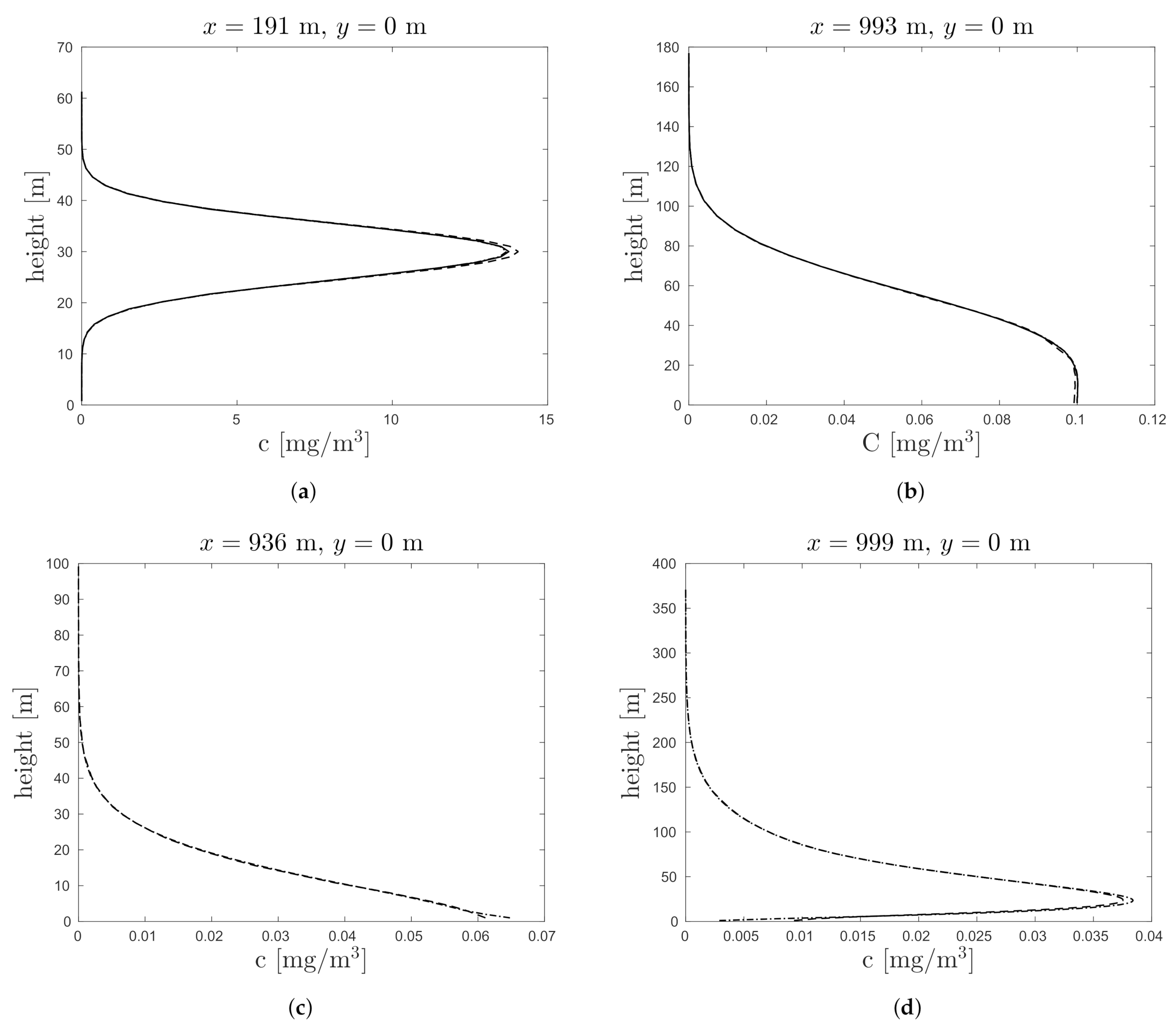
Figure 1. Concentration predictions due to an instantaneous point release by the PI (–) and KS (– –) estimator (np = 108 particles). Case I–HT (a) 20 s after release, (b) 104 s after release, exact solution (39) (–) also displayed. (c) Case I, 120 s after release. (d) Case III, 118 s after release.
Atmosphere 12 01343 g001
Figure 2. MISE against the released number of particles np for the PI and KS estimator in an unstable atmosphere at (a) 24 s and (b) 118 s after release, NR refers to normal reference rule and FD to the finite difference (see text). The lines represent the least-squares estimate of the corresponding MISE.
Atmosphere 12 01343 g002
Figure 3. Measured (∘) and predicted concentration profiles by the PI (–) and KS (– –) estimator during a stable stratification at the 100 m -arc for (a,b) experiment 22 (c,d) experiment 29 (e,f) experiment 40 with n p = 1000 particles per release time and Δ t * = 0.05 . For each experiment the vertical profile from the tower closest to the wind direction is shown.
Atmosphere 12 01343 g003aAtmosphere 12 01343 g003b
Figure 4. Measured (◦) and predicted concentration profiles by the PI (–) and KS (– –) estimator during an unstable stratification at the 100 m-arc for (a,b) experiment 15 (c,d) experiment 34 (e,f) experiment 61 with np = 1000 particles per release time and ∆t = 0.01. For each experiment, the vertical profile from the tower closest to the wind direction is shown.
Atmosphere 12 01343 g004
Table 1. Parameter values used in the convergence study to evaluate the parameterizations in Appendix A. The symbol ‘/’ indicates that the parameter is not required or that the value obtained from its parameterization is used. Case I–HT adopts the same parameter values as case I (see text).
CaseL (m) u * (m s 1 ) κ (-) σ u (m s 1 ) σ v (m s 1 ) h i (m) z 0 (m) h stack (m) Q 0 (kg)
I2480.380.35///0.008300.1
II530.240.350.590.38/0.008300.1
III 87 0.390.35//8360.008300.1
Table 2. Convergence study results. PI refers to estimator (24) and KS to (6). The case column refers to the cases in Table 1. Column h * displays the method to evaluate the Laplacian in the bandwidth of kernel K 1 in Equations (37) and (38): NR refers to normal reference rule (13) and FD to finite differences. The time column gives the simulated time at which the MISE is calculated. Columns β 0 and β 1 display the estimated coefficients from Equation (41). Column R 2 displays the R-squared value of the fits.
CaseMethod h * Time (s) β 0 β 1 R 2 (-)
I–HTPINR20 0.68 5.340.99
NR104 0.76 3.311.00
KSNR20 0.60 6.021.00
NR104 0.60 3.951.00
IPINR20 0.75 5.291.00
NR120 0.62 3.441.00
FD120 0.49 3.331.00
KSNR20 0.50 5.221.00
NR120 0.52 3.551.00
FD120 0.49 3.531.00
IIPINR27 0.77 5.511.00
NR156 0.70 4.201.00
FD156 0.77 4.261.00
KSNR27 0.56 5.771.00
NR156 0.44 4.170.99
FD156 0.50 4.121.00
IIIPINR24 0.81 5.991.00
NR118 0.52 3.311.00
FD118 0.79 3.971.00
KSNR24 0.59 5.251.00
NR118 0.37 3.200.99
FD118 0.44 3.480.99
Table 3. Values of the integrated Laplacian squared in Equation (8) for the bandwidth of kernel K 1 in Equations (37) and (38) with finite differences (FD) or the normal reference rule (NR). The case column refers to the case in Table 1. The time column gives the simulated time at which the integral is calculated.
CaseTime (s)FD (m 5 )NR (m 5 )
I–HT204.5 × 10 5 4.8 × 10 5
I1201.05 × 10 9 6.4 × 10 9
II1562.4 × 10 7 5.1 × 10 8
III1181.0 × 10 6 1.3 × 10 9
Table 4. Convergence test, comparison of c ^ ( Δ t * / 2 , 50 n p ) and c ^ ( Δ t * , n p ) . Stable: experiments 22, 29 and 40 with n p = 1000 particles per release time and Δ t * = 0.05 . Unstable: experiments 15, 34 and 61 with n p = 1000 particles per release time and Δ t * = 0.01 .
StratificationMethodMARE (%)FB (%)FAC1.05 (%)Number of Data Points (#)
stablePI12 0.71 58370
KS61 3.0 22408
unstablePI58 8.3 11939
KS147 9.0 5.61135
Publisher’s Note: MDPI stays neutral with regard to jurisdictional claims in published maps and institutional affiliations.