Abstract
Air pollution is a major health risk factor worldwide. Regular short- and long-time exposures to ambient particulate matter (PM) promote various diseases and can lead to premature death. Therefore, in Germany, air quality is assessed continuously at approximately 400 measurement sites. However, knowledge about this intermediate distribution is either unknown or lacks a high spatial–temporal resolution to accurately determine exposure since commonly used chemical transport models are resource intensive. In this study, we present a method that can provide information about the ambient PM concentration for all of Germany at high spatial (100 m × 100 m) and hourly resolutions based on freely available data. To do so we adopted and optimised a method that combined land use regression modelling with a geostatistical interpolation technique using ordinary kriging. The land use regression model was set up based on CORINE (Coordination of Information on the Environment) land cover data and the Germany National Emission Inventory. To test the model’s performance under different conditions, four distinct data sets were used. (1) From a total of 8760 (365 × 24) available h, 1500 were randomly selected. From those, the hourly mean concentrations at all stations (ca. 400) were used to run the model (n = 566,326). The leave-one-out cross-validation resulted in a mean absolute error (MAE) of and a root mean square error (RMSE) of . (2) For a more detailed analysis of how the model performs when an above-average number of high values are modelled, we selected all hourly means from February 2011 (n = 256,606). In February, measured concentrations were much higher than in any other month, leading to a slightly higher MAE of and RMSE of , respectively. (3) To enable better comparability with other studies, the annual mean concentration (n = 413) was modelled with a MAE of and a RMSE of . (4) To verify the model’s capability of predicting the exceedance of the daily mean limit value, daily means were modelled for all days in February (n = 10,845). The exceedances of the daily mean limit value of 50 were predicted correctly in 88.67% of all cases. We show that modelling ambient PM concentrations can be performed at a high spatial–temporal resolution for large areas based on open data, land use regression modelling, and kriging, with overall convincing results. This approach offers new possibilities in the fields of exposure assessment, city planning, and governance since it allows more accurate views of ambient PM concentrations at the spatial–temporal resolution required for such assessments.
1. Introduction
More than 40 years after the Geneva Convention on Long-Range Transboundary Air Pollution (CLRTAP) was signed, ambient air pollution is still a major cause of death and disease in the United Nations Economic Commission for Europe (UNECE) region and one of the most important health risk factors globally [1,2]. An estimated four million attributable premature deaths were linked to ambient air pollution in 2016, according to the World Health Organization, Geneva, Switzerland (WHO) [1]. For Europe, for the EU-28 countries, the European Environment Agency, Copenhagen, Denmark (EEA) reported 456,000 premature deaths attributable to ambient air pollution in 2016 caused by PM2.5, NO2, and O3 with 374,000 attributable to PM2.5, 68,000 to NO2, and 14,000 to O3 [3]. In this study, we considered PM10 due to the higher relevance and number of attributable premature deaths caused by particulate matter (PM). Since there is no legal limit value for hourly PM2.5 concentrations, the monitoring network is not as dense as PM10. Therefore, the long time series measurements for PM2.5 are limited [4], inhibiting a detailed study based on this quantity. PM10 is used instead. NO2 was not considered because, unlike PM10, it has few sources and high concentrations mainly occur in the direct vicinity of emissions. O3 was not considered in this study because to our knowledge land use regression (LUR) models cannot sufficiently represent the underlying complex photochemical processes [5,6,7].
Short- and long-term exposures to ambient air pollution can cause and promote diseases of the respiratory tract, such as a reduction of the overall lung function, aggravated asthma, and chronic obstructive pulmonary disease (COPD) [2,8]. Ultrafine particulate matter (UFP) of aerodynamic diameters smaller than 100 nm can penetrate deep into the lung passageways and enter the bloodstream, causing cardiovascular and cerebrovascular impact through stroke, heart disease, mutation, and abnormal growth of cells leading to cancer [9,10,11,12]. The highest exposure levels often occur in urban agglomerations due to high local emissions [13], making air pollution policy a major concern in different levels of governance [14] ranging from local administration [15] to international bodies of cooperation [3].
In 2016, 91% of the world population lived in areas where levels of the WHO air quality guidelines were not met [1]. According to these guidelines, the mean of particulate matter with a diameter of 10 microns or less (PM10) should not exceed 15 annually and 45 within 24 h [16]. In the European Union, the legal framework concerning air quality is set by the directive 2008/50/EC on ambient air quality and cleaner air for Europe [17]. Its daily limit value for PM10 of 50 is allowed to be exceeded 35 times within a calendar year, whereas the annual limit value is set to 40 .
Although air quality is measured continuously at many locations, its overall spatiotemporal distribution often remains unknown because the information of a measured value at a certain location is limited to a certain representative area given by the siting-type of the measurement station [18]. To estimate area-wide ambient air concentrations, different methods and models are used. Spatiotemporal models with high resolutions can also increase the precision of address-level exposure estimations [19].
Chemistry transport models (CTM) solve numerous complex equations based on assumptions considering chemical and physical processes, such as transformation and deposition within the atmosphere. Due to their high demand for computational power, their spatial (horizontal) resolutions are relatively coarse and, thus, high temporal resolutions only allow the modelling of background concentrations [20]. Their respective edge lengths range from ca. 500 m to over 1–5 km up to (6.5 × 13 ). Using global CTM to estimate PM2.5, the coarse resolutions lead to underestimations of health impacts in densely populated and industrialised areas [21]. The Copernicus Atmosphere Monitoring Service (CAMS) of the European Centre of Medium-Range Weather Forecasts, Reading, UK (ECMWF) provides free accessible hourly air pollution analyses and forecasts for Europe at a spatial resolution of based on an ensemble model [20,22,23,24]. It combines nine state-of-the-art numerical air quality models developed in Europe, including, e.g., CHIMERE [25] and LOTOS-EUROS [26]. For modelling air quality at the national scale, the German Environment Agency (Umweltbundesamt, UBA) uses the model REM-CALGRID (RCG), developed by Stern [27]. Land use regression models are alternative and widely used approaches for modelling pollutant concentrations in ambient air [28,29].
In contrast to CTM, they allow real-time assessments of ambient air quality at fine spatial–temporal scales of hourly mean values and a horizontal spatial resolution up to a few meters. So far this has mostly been conducted for individual cities, e.g., Zurich, Switzerland [30], Quebec, Canada [31], Calgary, Canada [32], London, UK [33], or Hong Kong, China [34]. Such models are not easy to adapt to different regions because of the different variables used as predictors in land use regression models, statistically-tuned parameters, and the availability of data sets describing these. Parameters often used in LUR models are related to information about land use or land cover, building density or building height, and the configuration of streets. When this approach is extended to a region or country level, the resolutions in space and time typically become coarser, down to annual mean values of some square kilometres. Ultimately, such LUR modelling then shows the same limitations as CTM [35,36].
In this study, we follow the hypothesis that the gap can be closed by applying the LUR model technique using only free and European-wide available open source data to model hourly real-time ambient air pollution of PM10 in Germany with a horizontal spatial resolution of 100 × 100 m efficiently and at acceptable accuracy. For this purpose, we adopted and modified the method from Janssen et al. [37] in connection with Hooyberghs et al. [38] and Knörchen et al. [39] for its application in Germany. The modelled PM10 concentrations allow more exact quantifications of the population’s exposure (both in space and time). The model combines a geostatistical method (ordinary kriging) and land use regression to predict the hourly mean concentration of PM10 with a spatial resolution of 100 × 100 m². The prediction is based on the CORINE land cover (CLC) dataset from the European Commission, the German National Emission Inventory, and quality assured PM10 measurements from over 400 stations of Germany’s air quality monitoring network. A total of four different data sets were used. (1) From a total of 8760 (365 × 24) available hours, 1500 were randomly selected. The hourly mean concentrations at all stations (ca. 400) were used to optimise the actual model (n = 566,326). (2) For a more detailed analysis, all hourly means of February 2011 (n = 256,506) were selected to examine the impact of episodes of high concentrations lasting several days on the model performance. (3) To enable better comparability with other studies, the modelled annual means of all stations were further investigated (n = 413). (4) To verify the model’s capability of predicting the exceedance of the daily mean limit value of 50 , daily means were modelled for all days in February (n = 10,845). After presenting data and methods in the following section, we then report on the results. An in-depth discussion of the results is followed-up with the overall conclusions.
2. Materials and Methods
2.1. Study Area
The topography and altitude of Germany are rather moderate, apart from some low mountain ranges and a part of the European Alps in the south of Germany. The average altitude calculated from the digital elevation model of Germany with a cell size of 200 m × 200 m is 250 m [40]. The range spans from −3.5 to 2962 m. The climate is temperate and westerly winds are predominant. According to the effective climate zones defined by Köppen-Geiger in Eastern Germany, the moist and warm continental climate (type: Dfb) is predominant. The western parts are classified as sea climate (type: Cfb) [41]. Of Germany’s population, 77% live in urban areas [42]. Urban fabrics hold a share of the surface area of 5 % followed by roads (8%), pastures (16%), forests (29%), and arable land (34%). Figure 1 shows the corresponding CORINE land cover and the locations of the air quality measurement stations used in this study.
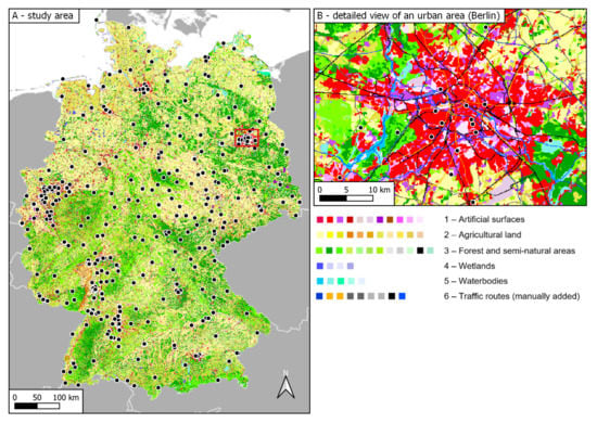
Figure 1.
CORINE land cover in Germany (A), the metropolitan area of Berlin (B), and the locations of air quality stations (black dots) used in this study. Legend items are grouped by the first level of the official CORINE land cover class nomenclature. Each element within a group represents a third-level CORINE land cover class. A full legend with all items is provided in Appendix A. The items belonging to the first level 6 class (traffic routes) are only visible in map (B). The brown areas in the southwestern part of map (A) correspond to the third-level classes, 221 (vineyards) and 222 (fruit trees and berry plantations) belonging to the first level 2 class (Agricultural land).
2.2. Datasets and Preprocessing
As a basis for the interpolation, we chose hourly means of PM10 concentrations retrieved from the air quality monitoring network of the 16 German states and the UBA’s six background measurement stations in 2011. These data are freely available upon request from the German Environment Agency. Due to the frequent occurrences of cold and atmospherically stable high-pressure weather conditions [43], the measured PM10 concentrations in 2011 exceeded the daily mean limit value of 50 more often compared to any other year since the directive 2008/50/EC on ambient air quality and cleaner air for Europe [17] came into effect in 2008 (Figure 2). Although the limit value had already existed since 2005, it did not have to be actually complied with until 2011 following an extension of the deadline in Germany. The legal situation in force today was therefore applied for the first time in the year 2011. To investigate how the model performance differs under varying conditions, we specifically chose the year 2011. Out of all data in 2011, subsets (1) to (4) were derived as described in the introduction.
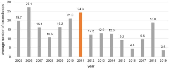
Figure 2.
Average number of exceedances per active station of the daily mean limit value of 50 set by the directive 2008/50/EC on ambient air quality and cleaner air for Europe [17].
The land cover is represented by the CORINE land cover 10 dataset (CLC10) from 2012, available at the Federal Agency for Cartography and Geodesy of Germany (Bundesamt für Kartographie und Geodäsi, BKG). It represents a description of the landscape that reflects land cover and it includes aspects of land use. The basis for CLC10 is the land cover model for Germany, 2012 (LBM-DE2012), with its detailed classification into land cover and land use with a minimum size of 1 ha (100 by 100 m). Combining that information, unique CLC classes were derived. The downloaded vector data set was rasterised with a cell size of 100 by 100 m.
Data on emissions were generated using GRETA, the tool customarily applied in Germany for the nationwide gridding of emissions [44]. The dataset contains the sum of the annual primary PM10 emissions in Germany for the year 2011 as submitted in 2018 under the Geneva Convention on Long-Range Transboundary Air Pollution of the United Nations Economic Commission for Europe (CLRTAP/UNECE) as well as the National Emission Ceiling (NEC) directive of the European Union with a spatial resolution of 500 by 500 m. The 2018 submission is the first including PM10 emissions on railways from abrasion and wear [45], leading to an increase from to 8 in that sector compared to the previous 2017 submission, which was very important for the correct distribution of emissions to the land cover classes. These data are freely available upon request from the German Environment Agency.
Hourly means were not available for most of the stations in the state of Baden-Württemberg, since they were only measured gravimetrically according to the British Standard Institution procedure BS EN 12341:1999 [46], resulting in daily mean values. In order to retrieve hourly mean concentrations for those locations, we calculated mean daily cycles based on hourly data from all stations in the neighbouring states Rhineland-Palatinate, Hesse, and Bavaria. The hourly values for stations in Baden-Württemberg were then calculated based on their respective daily mean and the relative fraction according to the overall average daily cycle on that day in neighbouring states.
CLC data sets were complemented with nine additional third-level classes representing traffic paths, such as motorways, highways, district roads, railways, and waterways because of their high importance for ambient PM10 concentrations (Figure 3). Following the logic of the CORINE class nomenclature, they constitute a new first-level class 6 (traffic routes), including three new second-level classes, i.e., classes 61 (roads), 62 (railways) and 63 (waterways). The all-new level 3 classes (611–631) are displayed in Figure 3 and Appendix A. The data were provided by the Federal Agency for Cartography and Geodesy of Germany but can also be obtained freely in similar good quality from OpenStreetMap [47].
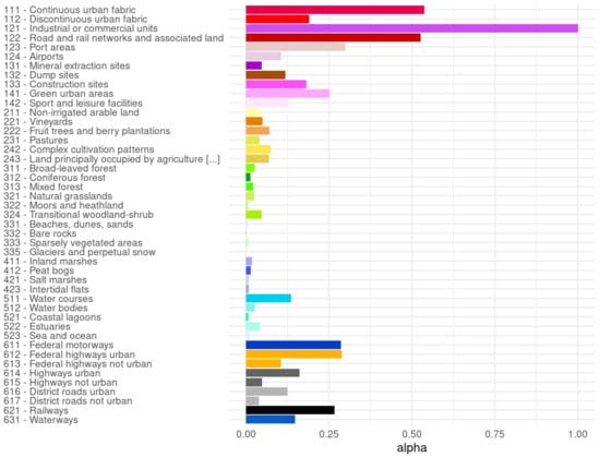
Figure 3.
Level 3 CORINE land cover classes with their number, name, and emission land use coefficient (alpha). Classes 611–631 were manually generated and added (see Section 2.2).
2.3. Geostatistical Modelling
Measurements from air quality networks innately show different features depending on their surroundings and, therefore, siting-type (e.g., traffic, industry, background). PM concentrations at traffic sites typically show higher concentrations than monitoring stations located in the rural background. These site-specific characteristics needed to be removed before data are used in the kriging procedure. Details on the principles of the methodology can be found in Hooyberghs et al. [38] and Janssen et al. [37].
To set up a function to remove the siting-type character of the measured values, the emissions from GRETA of a pixel i are assigned to the CORINE land cover class via a spatial overlay of the two raster data sets resulting in a set of pixels belonging to this class. The average PM10 emission of a CORINE land cover class is calculated by
is the number of pixels in . Then the land use emission coefficient of a CORINE land cover class is given by the average PM10 emission normalised by the maximum average PM10 emission of all classes:
To describe the character of a station, the land use emission coefficient is allocated to each pixel i depending on its land cover class: . The station-related emission coefficient is then given by the average within a certain radius depending on the siting-type of the station (Table 1):

Table 1.
Buffer radii configurations according to Annex III of the directive 2008/50/EC for different siting-types and their surrounding areas.
Here, is the buffer around the station, and is the number of pixels. The ranges from 0 to 1. Linear regression with the logarithm of as a predictor for the measured annual mean PM10 concentration in 2011 of each station () results in R² = 0.32 with a constant of and a slope of :
Analogous to Janssen et al. [37], this regression function to be applied to the station data is called the “de-trending function” hereafter. Consequently, and also after Janssen et al. [37] applying its inverse formulation to the entire grid, it is denoted as “re-trending”, despite the fact that it does not explicitly model temporal or spatial trends but the characteristics according to the station location or land use classes. Following this notion, prior to the spatial interpolation with ordinary kriging, the de-trending function
is applied to the observations and transmutes all values to a reference level by adding the difference between a constant arbitrary target value c and the value of the de-trending function for the respective of the station to the original value . For the operational use of the model, c was set to 70 . We also tried other values but the metrics of the leave-one-out cross-validation did not change or improve.
The model for the spatial interpolation with ordinary kriging was built in R (version 4.1.1) [48] using the package “gstat” [49]. For each time step, an exponential semi-variogram was fit to the de-trended values. The search neighbourhood was split into four sectors of 90 ° each (north: 315° –45°, east: 45°–135°, south: 135°–225°, and west: 225°–315°). For each sector, an individual semi-variogram was computed. The sectors are used to account for the potential influence of the wind direction on the measured PM10 concentrations. The average distance between stations was approximately 18 km. Therefore, kriging was performed at a horizontal resolution of 1 × 1 only. After, the interpolation procedure grid resolution was resampled to 100 by 100 m. To receive the real-world values for the entire grid based on the CORINE land cover class, the still de-trended values from the kriging procedure needed to be re-trended by applying the re-trending function
3. Results
To find the best settings to model the hourly mean concentration in Germany with a spatial resolution of 100 by 100 m, we adjusted the model parameters stepwise (Table 2) and carried out a leave-one-out cross-validation (loo-cv) for each run with dataset (1). In contrast to the model itself, which only took about five minutes to return its results, the loo-cv was compute-intensive. Thus, we parallelised the procedure on a high-performance computing cluster. This reduced the required time for one run, including the loo-cv from 4.5 years to only 4 days, making this analysis possible in the first place.

Table 2.
Parameter adjustments and corresponding metrics of the leave-one-out cross-validation (loo-cv) of all runs during the optimisation process with dataset (1) (MAE and RMSE in .)
For the initial run (run 1), a fixed buffer radius of 3 km was used as a starting point in the optimisation process. Increasing the size of the buffer from 2 km used in the study of Janssen et al. [37] led to a higher R² of the trend function. We also distributed the emissions from facilities in the point release and transport register (PRTR) areal with GRETA [44] (run 2), meaning that the emissions from a point source were assigned to the raster cell the source was located in. We further capped the emissions at the 99.99% percentile (run 3) to avoid a disproportionate influence of single large emitters on a specific CORINE land cover class. The greatest improvement was achieved in run 4 by changing the buffer radius from a fixed value of 3 km to individual radii, depending on the siting-type of the station (traffic, industrial, background) and its surrounding area (urban, suburban, rural) to calculate the value of that station. The radii were set according to Annex III of the directive 2008/50/EC on ambient air quality and cleaner air for Europe [17] (Table 1). The nine additional CORINE land cover classes (traffic routes) described above were implemented in run 5. In run 6, the trend functions were optimised by using the logarithm of the values. Values higher than the 99.99% percentile of all measured values were excluded from drawing a new random sample for the loo-cv in run 7. This prevented implausible values caused by single extreme events, such as large construction sites next to a monitoring station, distorting the loo-cv, as in Glauchau, Saxony (station code: DESN019). The model configuration of run 7 was used further. To analyse the effects of different regional concentration levels caused by different contributions of secondary particles on the model performance, a constant increment of 10 was added to all measurement values in run 8.
The chosen settings in run 7 with dataset (1) led to an overall good model performance with a strong correlation between the observed and modelled values (R² = 0.80). The mean absolute error (MAE) and the root mean square error (RMSE) were and , respectively. The median and the mean of the residuals were close to 0, indicating the absence of any bias. In fact, 98% of all residuals were within the range of approximately ± 30 (Table 3).

Table 3.
Results of the leave-one-out cross-validation (loo-cv) for the different datasets used (MAE, RMSE, and residuals in ).
However, when extreme values were modelled, there was a tendency to underestimate very high and to overestimate very low values (Figure 4). Although the metrics were very similar to all station types, there was a slight overestimation at background stations whereas values at traffic stations were underestimated. The utilisation of the synthesised hourly mean concentrations for the traffic sites in Baden-Württemberg were not reflected in the loo-cv results, since MAE and RMSE were very similar for both types of data, measured and synthesised (Table 4).
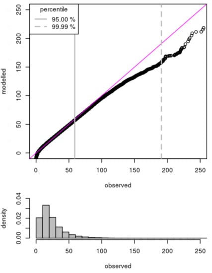
Figure 4.
The Q-Q plot and histogram of the observed and modelled values of run 7 with dataset (1) with the 95 % (solid line) and 99.99 % (dashed line) percentile of measured values within the dataset (1).

Table 4.
Leave-one-out cross-validation (loo-cv) results of run 7 with dataset (1) concerning the type of station and the type of data (MAE, RMSE, and median in ).
The model performance varies depending on the hour of the day and the season. The best predictions are obtained in the summer. Deviations are generally higher during rush hours (Figure 5).
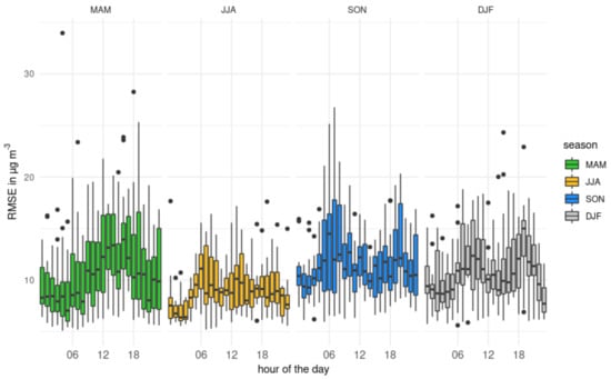
Figure 5.
Root Mean Square Error (RMSE) boxplots of the leave-one-out cross-validation (loo-cv) of run 7 with dataset (1) depending on the hour of the day and the season.
In terms of spatial variations, the model performs equally well in rural regions as in urban and densely populated areas (Figure 6). However, five locations (highlighted on the map with a station code label) showed difficulties that the model was not able to compensate for, resulting in a high RMSE; these were:
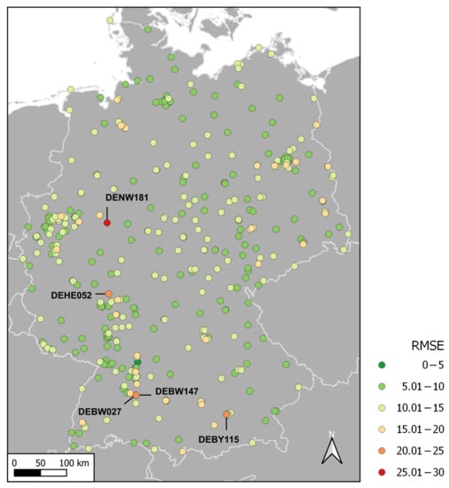
Figure 6.
Spatial distribution of the air quality monitoring stations and their RMSE from the loo-cv in from run 7 with dataset (1). Stations are labelled with their station codes when their RMSEs were above 20 .
- The proximity of monitoring stations of different types, especially background and traffic, causing high differences in the loo-cv procedure in the case where one of the two stations was left out,
- The recurrence of single events in the vicinity of the measurement station with strong impacts on PM concentrations at this station, causing very high measured values, which the model was not able to reproduce accurately, and
- A false prediction based on the value used in the re-trending process due to discrepancies between the CORINE land cover classification and the real-world conditions.
For a more detailed analysis of the model’s performance with the final parameter settings from run 7, we selected all hours from February 2011 (dataset (2)). February was the month with the most limit-value exceedances in 2011 and had the highest monthly mean concentration with . The lowest monthly mean concentration was measured in July with . The annual mean in 2011 was . The loo-cv results of dataset (2) showed that the model’s application to episodes of high concentrations led to higher error rates (Table 3). After the aggregation to daily means (dataset (4), n = 10,845), it was tested whether the daily mean limit of 50 was reached or not. The result was then compared to the observed values. In 5.90% of all cases, the model predicted an exceedance although there was none, in 5.43% an existing limit exceedance was not captured by the model leading to an overall hit rate of 88.67%.
Modelling the annual mean concentration (dataset (3), n = 413), with which the trend function was fit, the MAE and RMSE improved to and .
4. Discussion
The overall performance of the presented model is comparable with previously published results from other models using land-use information. The model performance varies with respect to the temporal resolution between annual and daily averages. The model presented here shows better performance for hourly datasets according to R² whereas MAE and RMSE show better values for the annual dataset.
For daily averages, Janssen et al. [37] reported values for RMSE of and for MAE of with a similar model that compares well to our results. For annual averages in a European-wide model approach using urban land zone(s) (ULZ), Diaz-de Quijano et al. [50] found an R² of 0.49 and a RMSE of . A study assessing air pollution exposure in the Mexico City Metropolitan Area (with a land-use regression model) showed the same effects of different temporal resolutions on R² and RMSE as our study, with values for R² and RMSE of 0.38 and , respectively, for the hourly values [51]. Merging land-use information with satellite-based data for aerosol optical depth (AOD) and meteorological data, however, can improve model performance with respect to R² for annual means in China (R² = 0.81) [52]. Nevertheless, such improvements did not occur with respect to RMSE, which was even higher at in the study by Chen et al. [52] than the RMSE for the least predictable month (February) in our study. Table 5 provides an overview of the compared models and their results.

Table 5.
Summary of the model results from similar studies with their respective study period and area plus their spatial–temporal resolution (Res.) (MAE and RMSE in ).
The variations of the model performance due to seasonality and hour of the day suggest the need for a better data basis (in terms of the emission inventory). Since the trend function is based on the annual sum of primary emissions, time-dependent differences in hourly measured values cannot be considered in the trend function. Diurnal variations are mainly caused by traffic during commuting hours and differ between working days and weekends. Seasonal variations, on the other hand, are triggered by meteorological conditions and domestic heating, especially in rural areas [53,54]. With finer temporal resolutions of the emission inventory data, trend functions for each season, month, day of the week, or time of day, could be created and implemented.
Considering emission data, the applied approach is based solely on the spatial distributions of primary emissions. However, ambient particles also consist of variable and significant fractions of secondary particles. For example, secondary inorganic aerosols can contribute up to 50% of concentrations in northwestern Europe during high concentration episodes [55]. A study by Metz in the northeast of France shows that secondary organic aerosols can contribute about 22% to concentrations [56]. Secondary particles are not included when using an emission inventory for primary emissions since they are formed by gaseous precursors in the atmosphere. However, these particles are part of the measured concentrations. Due to their secondary formations, these particles show regional distribution patterns. Therefore, regional modelling approaches can use primary emissions to obtain the urban increments though it can be a simplification to assume that secondary particle formation at the local scale is negligible [57]. A constant increment of 10 to all measured values to test the effects of changes in regional concentration levels showed no impact on the loo-cv metrics and residual statistic. We concluded that the impacts of secondary particles at the regional level were well captured by the model.
Another limitation of the trend function was revealed in the loo-cv of dataset (1) and confirmed when we tested the model’s application to predict limit exceedances with dataset (4). Although the hit rate of almost 90% was relatively high nationwide, there were a set of stations for which the model’s results were not accurate. Those stations have one or more other stations of different siting-types in their proximities. In the city of Munich (Figure 7), the triangle of the straight-line distance between three stations, including DEBY115 (Figure 6), is only 6 km. This problem mostly occurs in urban areas where monitoring stations are clustered and at least one of them is of siting-type traffic. Deterministic CTM, such as LOTOS-EUROS and COSMO-CLM, usually neglect traffic monitoring sites as they are not representative for their model resolution [58].
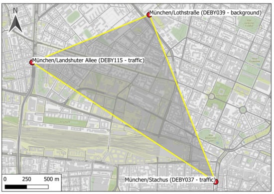
Figure 7.
Triangle connecting three closely-located air quality measurement stations of different siting-types in the centre of Munich. Map tiles by Stamen Design under CC BY 3.0. Data by OpenStreetMap [47] under ODbL.
In the city of Reutlingen, the distance between the background station DEBW027 and the next traffic station DEBW147 (Figure 6) is only 260 m. This shows that the trend function cannot completely (but only to some extent) eliminate the characteristics based on the station type within the values measured at that location. Therefore, we recommend adding a minimum distance between stations as a requirement for models using observations when defining siting criteria for sampling locations, as mentioned in Annex III of the directive 2008/50/EC on ambient air quality and cleaner air for Europe [17]. This would improve the performances of such geostatistical models and lead to more common applications of these models.
Very high values cannot be modelled accurately. This is especially evident when single events with extraordinarily high concentrations reoccur at specific stations only. This led to an extreme high RMSE at the station in Warstein (DENW181) (Figure 6) where the model performs very well on average with a median of the residuals of only . However, on 21 April 2011, the station observed an hourly mean of whereas the model predicted only . Investigations have shown that on this date a huge cargo train with a diesel engine passed by on the railroad tracks only 30 m away from the monitoring station. Similar events presumably reoccurred due to the abnormally high values, especially during morning hours at this specific station. The problem of overall discrepancies at high concentrations could possibly be limited by a bias correction procedure, such as quantile mapping on the residuals. Using such an approach, the general error could be identified and calculated based on large time series. However, singular events with instantaneous and local characteristics cannot be eliminated since such geostatistical interpolation techniques cannot deal with individual single outliers.
The CORINE land cover product is a widely used dataset and its biggest advantages are its comprehensive consistency and its availability (i.e., being free of charge) [59]. Using the correlation between land use and PM concentration is a commonly used approach [50,60,61]. However, the 10 spatial resolution of the data on which it is based are quite coarse. This sometimes leads to classifications deviating from real-world conditions. The monitoring station on the mountain Kleiner Feldberg (DEHE052) (Figure 6) in the Taunus low mountain range is located at 811 m altitude next to an observatory and surrounded by dense forest. However, this surrounding is classified as “industrial or commercial units” on an area of 10 in the CLC10 data set. This class has the land use emission coefficient of 1 and, thus, leads to a systematic overestimation at that station, resulting in a higher RMSE. Despite such minor deficiencies, the availability of the CORINE land cover product is the preferred land use database since it allows the adaptation of the method to other countries in Europe, provided that the spatial distribution of the emission inventory is available at a comparable accuracy and spatial resolution.
Since the model uses the spatial distributions of primary emissions, one criterion for its applicability to other regions or countries might be the density distributions of the spatial emissions. Hence, Figure 8 shows the density functions of spatial emissions for the EU-27 member states. Most of these distributions peak at around 1000 per 49 km2, including Germany. However, while most countries show a unimodal distribution, the density distributions of emissions in Germany peak twice with a minor peak at 1 per 49 km2. We assume that countries with similar economic and population patterns have comparable density distribution functions. How different forms of the density distributions influence the model performance—and if this would require modifications to the model’s parametrisation for different countries—could be investigated in further research.
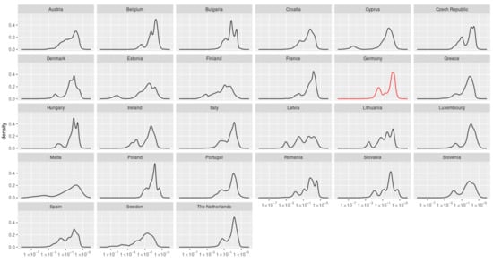
Figure 8.
Density functions of the spatially distributed emissions 2010 from the MACC-III (Monitoring Atmospheric Composition and Climate) project by the European Union in kilotons per 7 ×7 km2 (-scaled abscissa) in the EU-27 member states based on data from the Netherlands Organisation for Applied Scientific Research (TNO). Germany is highlighted with a red density function.
Other criteria we expect to influence the model results include the climate and its heterogeneity within the model domain. Moreover, large gradients within the landscape, such as on coasts or areas where mountain ranges are adjacent to the flat mountain foreland, are likely to adversely impact the model performance.
5. Conclusions
This study shows that it is possible to model the distribution of particulate matter at a high spatial–temporal resolution with acceptable restrictions solely with open data and freely available software. Such high spatial–temporal resolution is in stark contrast to the coarse spatial–temporal resolution of deterministic regional CTM currently used [20,24,62]. The high temporal resolution also allows for real-time air quality assessment. This can be used for more precise information for high-risk populations and the overall exposure in general, and further sensitise people to the issue of air pollution and public health [63,64]. The high spatial resolution allows for a more accurate exposure assessment and estimation of the burden of disease/other epidemiological studies [65,66]. The use of data, the collection and provision of which are mandatory within the European Union, extends the value chain of point-based data collected within the air quality monitoring station networks, which makes their operation more cost-effective for the member states. Since the method does not involve significant costs, it promotes the adaptation of the approach to other countries, states, municipalities, and cities to assess their regional or local air quality for both rural and urban areas. This is reinforced by the model’s independence from the level of the regional concentration. The possible temporal–spatial aggregation makes the scheme very flexible and provides a powerful tool for urban planners, policy makers, and governments. Within the parameter optimisation procedure, it was found that adjusting the buffer size, depending on the siting-type of the station, resulted in better values of MAE, RMSE, and R² returned by the leave-one-out cross-validation. On the one hand, this adjustment improves the performance of the model and, at the same time, reflects the legal and content-related requirements for the configuration and representativeness of air quality measurement stations. The model could be easily improved by employing emission data with higher temporal resolution than annual sums only. Moreover, the use of regression-kriging with altitude as an auxiliary variable could improve the results and should possibly be considered, especially in more mountainous terrain. How relief and climate and their spatial gradients within the study area affect the model needs to be investigated in more detail. Due to its characteristics, this model is very well suited to assimilate currently measured or predicted PM concentrations. Predictions of PM concentrations can be generated by applying machine learning techniques in combination with satellite data or the output from numerical weather prediction models [67,68,69,70,71]. Such a combination would allow a retrospective assessment of the air quality (as in this study) as well as prospective information of both authorities and the general public. They could then prepare themselves for the expected situation. Thus, exposure to high PM concentrations could be effectively reduced. Further, peak concentrations might be prevented through the initiation of recommendations and measures beforehand.
Author Contributions
Conceptualisation, S.W., M.L., and C.S.; methodology, S.W., M.L., and C.S.; software, S.W. and S.S.; validation S.W. and M.L.; formal analysis, S.W.; investigation, S.W.; resources, S.S.; data curation, S.W.; writing—original draft preparation, S.W. and M.L.; writing—review and editing, S.W., M.L., S.S., and C.S.; visualisation, S.W.; supervision, M.L. and C.S.; project administration, S.W. All authors have read and agreed to the published version of the manuscript.
Funding
This research received no external funding.
Institutional Review Board Statement
Not applicable.
Informed Consent Statement
Not applicable.
Data Availability Statement
The data presented in this study are available upon request from the corresponding author.
Acknowledgments
Stefan Feigenspan is greatly acknowledged for sharing his valuable thoughts on the concept of this work, as well as his technical support and data provisioning. We thank Stephan Nordmann very much for his helpful hints and insights, especially regarding the validation process. We are deeply indebted to Daniel Roob for his thorough proofreading of the manuscript. The authors of this manuscript would also like to thank the two anonymous reviewers for their insight, helpful comments, and valuable advice.
Conflicts of Interest
The authors declare no conflict of interest.
Appendix A
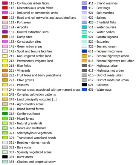
Figure A1.
Colour, number, and name of all level 3 CORINE land cover classes (classes 611–631 were manually added).
References
- World Health Organization. Ambient Air Pollution: A Global Assessment of Exposure and Burden of Disease; WHO: Geneva, Switzerland, 2016. [Google Scholar]
- Watts, N.; Amann, M.; Arnell, N.; Ayeb-Karlsson, S.; Belesova, K.; Boykoff, M.; Byass, P.; Cai, W.; Campbell-Lendrum, D.; Capstick, S.; et al. The 2019 report of The Lancet Countdown on health and climate change: Ensuring that the health of a child born today is not defined by a changing climate. Lancet 2019, 394, 1836–1878. [Google Scholar] [CrossRef]
- European Environment Agency. Air Quality in Europe, 2019; European Environment Agency: Copenhagen, Denmark, 2019. [Google Scholar] [CrossRef]
- Eeftens, M.; Tsai, M.Y.; Ampe, C.; Anwander, B.; Beelen, R.; Bellander, T.; Cesaroni, G.; Cirach, M.; Cyrys, J.; de Hoogh, K.; et al. Spatial variation of PM2.5, PM10, PM2.5 absorbance and PMcoarse concentrations between and within 20 European study areas and the relationship with NO2—Results of the ESCAPE project. Atmos. Environ. 2012, 62, 303–317. [Google Scholar] [CrossRef]
- Huang, L.; Zhang, C.; Bi, J. Development of land use regression models for PM2.5, SO2, NO2 and O3 in Nanjing, China. Environ. Res. 2017, 158, 542–552. [Google Scholar] [CrossRef] [PubMed]
- Kerckhoffs, J.; Wang, M.; Meliefste, K.; Malmqvist, E.; Fischer, P.; Janssen, N.A.; Beelen, R.; Hoek, G. A national fine spatial scale land-use regression model for ozone. Environ. Res. 2015, 140, 440–448. [Google Scholar] [CrossRef]
- Malmqvist, E.; Olsson, D.; Hagenbjörk-Gustafsson, A.; Forsberg, B.; Mattisson, K.; Stroh, E.; Strömgren, M.; Swietlicki, E.; Rylander, L.; Hoek, G.; et al. Assessing ozone exposure for epidemiological studies in Malmö and Umeå, Sweden. Atmos. Environ. 2014, 94, 241–248. [Google Scholar] [CrossRef][Green Version]
- Siafakas, N.M.; Vermeire, P.; Pride, N.B.; Paoletti, P.; Gibson, J.; Howard, P.; Yernault, J.C.; Decramer, M.; Higenbottam, T.; Postma, D.S. Optimal assessment and management of chronic obstructive pulmonary disease (COPD). The European Respiratory Society Task Force. Eur. Respir. J. 1995, 8, 1398–1420. [Google Scholar] [CrossRef]
- Donaldson, K.; Li, X.; MacNee, W. Ultrafine (nanometre) particle mediated lung injury. J. Aerosol Sci. 1998, 29, 553–560. [Google Scholar] [CrossRef]
- Boffetta, P. Human cancer from environmental pollutants: The epidemiological evidence. Mutat. Res. Toxicol. Environ. Mutagen. 2006, 608, 157–162. [Google Scholar] [CrossRef]
- Valavanidis, A.; Vlachogianni, T.; Fiotakis, K.; Loridas, S. Pulmonary oxidative stress, inflammation and cancer: Respirable particulate matter, fibrous dusts and ozone as major causes of lung carcinogenesis through reactive oxygen species mechanisms. Int. J. Environ. Res. Public Health 2013, 10, 3886–3907. [Google Scholar] [CrossRef]
- Barrett, J.R. Assessing the health threat of outdoor air: Lung cancer risk of particulate matter exposure. Environ. Health Perspect. 2014, 122, A252. [Google Scholar] [CrossRef]
- Mayer, H. Air pollution in cities. Atmos. Environ. 1999, 33, 4029–4037. [Google Scholar] [CrossRef]
- Walters, R. Toxic Atmospheres Air Pollution, Trade and the Politics of Regulation. Crit. Criminol. 2010, 18, 307–323. [Google Scholar] [CrossRef]
- Grote, R.; Samson, R.; Alonso, R.; Amorim, J.H.; Cariñanos, P.; Churkina, G.; Fares, S.; Le Thiec, D.; Niinemets, Ü.; Mikkelsen, T.N.; et al. Functional traits of urban trees: Air pollution mitigation potential. Front. Ecol. Environ. 2016, 14, 543–550. [Google Scholar] [CrossRef]
- World Health Organization. WHO Global Air Quality Guidelines: Particulate Matter (PM2.5 and PM10), Ozone, Nitrogen Dioxide, Sulfur Dioxide and Carbon Monoxide; World Health Organization, WHO: Geneva, Switzerland, 2021; p. 19. [Google Scholar]
- European Commission. Directive 2008/50/EC of the European Parliament and of the Council of 21 May 2008 on Ambient Air Quality and Cleaner Air for Europe; European Union: Brussels, Belgium, 2008. [Google Scholar]
- Henne, S.; Brunner, D.; Folini, D.; Solberg, S.; Klausen, J.; Buchmann, B. Assessment of parameters describing representativeness of air quality in-situ measurement sites. Atmos. Chem. Phys. 2010, 10, 3561–3581. [Google Scholar] [CrossRef]
- Butland, B.K.; Samoli, E.; Atkinson, R.W.; Barratt, B.; Katsouyanni, K. Measurement error in a multi-level analysis of air pollution and health: A simulation study. Environ. Health Glob. Access Sci. Source 2019, 18, 13. [Google Scholar] [CrossRef]
- Schaap, M.; Cuvelier, C.; Hendriks, C.; Bessagnet, B.; Baldasano, J.M.; Colette, A.; Thunis, P.; Karam, D.; Fagerli, H.; Graff, A.; et al. Performance of European chemistry transport models as function of horizontal resolution. Atmos. Environ. 2015, 112, 90–105. [Google Scholar] [CrossRef]
- Kushta, J.; Pozzer, A.; Lelieveld, J. Uncertainties in estimates of mortality attributable to ambient PM 2.5 in Europe. Environ. Res. Lett. 2018, 13, 064029. [Google Scholar] [CrossRef]
- Kukkonen, J.; Olsson, T.; Schultz, D.M.; Baklanov, A.; Klein, T.; Miranda, A.I.; Monteiro, A.; Hirtl, M.; Tarvainen, V.; Boy, M. A review of operational, regional-scale, chemical weather forecasting models in Europe. Atmos. Chem. Phys. 2012, 12, 1–87. [Google Scholar] [CrossRef]
- Solazzo, E.; Bianconi, R.; Pirovano, G.; Matthias, V.; Vautard, R.; Moran, M.D.; Appel, K.W.; Bessagnet, B.; Brandt, J.; Christensen, J.H. Operational model evaluation for particulate matter in Europe and North America in the context of AQMEII. Atmos. Environ. 2012, 53, 75–92. [Google Scholar] [CrossRef]
- Prank, M.; Sofiev, M.; Tsyro, S.; Hendriks, C.; Semeena, V.; Vazhappilly Francis, X.; Butler, T.; van der Gon, H.D.; Friedrich, R.; Hendricks, J.; et al. Evaluation of the performance of four chemical transport models in predicting the aerosol chemical composition in Europe in 2005. Atmos. Chem. Phys. 2016, 16, 6041–6070. [Google Scholar] [CrossRef]
- Menut, L.; Bessagnet, B.; Khvorostyanov, D.; Beekmann, M.; Blond, N.; Colette, A.; Coll, I.; Curci, G.; Foret, G.; Hodzic, A.; et al. CHIMERE 2013: A model for regional atmospheric composition modelling. Geosci. Model Dev. 2013, 6, 981–1028. [Google Scholar] [CrossRef]
- Kranenburg, R.; Segers, A.J.; Hendriks, C.; Schaap, M. Source apportionment using LOTOS-EUROS: Module description and evaluation. Geosci. Model Dev. 2013, 6, 721–733. [Google Scholar] [CrossRef]
- Stern, R. Entwicklung und Anwendung des Chemischen Transportmodells REM/CALGRID; Umweltbundesamt: Dessau-Roßlau, Germany, 2003. [Google Scholar]
- Hoek, G.; Beelen, R.; de Hoogh, K.; Vienneau, D.; Gulliver, J.; Fischer, P.; Briggs, D. A review of land-use regression models to assess spatial variation of outdoor air pollution. Atmos. Environ. 2008, 42, 7561–7578. [Google Scholar] [CrossRef]
- Shafran-Nathan, R.; Etzion, Y.; Broday, D.M. Fusion of land use regression modeling output and wireless distributed sensor network measurements into a high spatiotemporally-resolved NO2 product. Environ. Pollut. 2020, 271, 116334. [Google Scholar] [CrossRef]
- Lautenschlager, F.; Becker, M.; Kobs, K.; Steininger, M.; Davidson, P.; Krause, A.; Hotho, A. OpenLUR: Off-the-shelf air pollution modeling with open features and machine learning. Atmos. Environ. 2020, 233, 117535. [Google Scholar] [CrossRef]
- Adam-Poupart, A.; Brand, A.; Fournier, M.; Jerrett, M.; Smargiassi, A. Spatiotemporal modeling of ozone levels in Quebec (Canada): A comparison of kriging, land-use regression (LUR), and combined Bayesian maximum entropy-LUR approaches. Environ. Health Perspect. 2014, 122, 970–976. [Google Scholar] [CrossRef]
- Bertazzon, S.; Johnson, M.; Eccles, K.; Kaplan, G.G. Accounting for spatial effects in land use regression for urban air pollution modeling. Spat. Spatio-Temporal Epidemiol. 2015, 14–15, 9–21. [Google Scholar] [CrossRef]
- Tang, R.; Blangiardo, M.; Gulliver, J. Using building heights and street configuration to enhance intraurban PM10, NO(X), and NO2 land use regression models. Environ. Sci. Technol. 2013, 47, 11643–11650. [Google Scholar] [CrossRef]
- Shi, Y.; Lau, K.K.L.; Ng, E. Developing Street-Level PM2.5 and PM10 Land Use Regression Models in High-Density Hong Kong with Urban Morphological Factors. Environ. Sci. Technol. 2016, 50, 8178–8187. [Google Scholar] [CrossRef]
- Sampson, P.D.; Richards, M.; Szpiro, A.A.; Bergen, S.; Sheppard, L.; Larson, T.V.; Kaufman, J.D. A regionalized national universal kriging model using Partial Least Squares regression for estimating annual PM2.5 concentrations in epidemiology. Atmos. Environ. 2013, 75, 383–392. [Google Scholar] [CrossRef]
- Ma, Z.; Hu, X.; Huang, L.; Bi, J.; Liu, Y. Estimating ground-level PM2.5 in China using satellite remote sensing. Environ. Sci. Technol. 2014, 48, 7436–7444. [Google Scholar] [CrossRef] [PubMed]
- Janssen, S.; Dumont, G.; Fierens, F.; Mensink, C. Spatial interpolation of air pollution measurements using CORINE land cover data. Atmos. Environ. 2008, 42, 4884–4903. [Google Scholar] [CrossRef]
- Hooyberghs, J.; Mensink, C.; Dumont, G.; Fierens, F. Spatial interpolation of ambient ozone concentrations from sparse monitoring points in Belgium. J. Environ. Monit. 2006, 8, 1129–1135. [Google Scholar] [CrossRef] [PubMed]
- Knörchen, A.; Ketzler, G.; Schneider, C. Implementation of a near-real time cross-border web-mapping platform on airborne particulate matter (PM) concentration with open-source software. Comput. Geosci. 2015, 74, 13–26. [Google Scholar] [CrossRef]
- Bundesamt für Kartographie und Geodäsie. Dokumentation Digitales Geländemodell Gitterweite 200 m: DGM200; Federal Agency for Cartography and Geodesy BKG: Frankfurt am Main, Germany, 2021. [Google Scholar]
- Beck, H.E.; Zimmermann, N.E.; McVicar, T.R.; Vergopolan, N.; Berg, A.; Wood, E.F. Present and future Köppen-Geiger climate classification maps at 1-km resolution. Sci. Data 2018, 5, 180214. [Google Scholar] [CrossRef]
- The World Bank. Urban Population. 2022. Available online: https://data.worldbank.org/indicator/SP.URB.TOTL.IN.ZS?locations=DE (accessed on 4 May 2022).
- Umweltbundesamt. Luftqualität 2011: Feinstaubepisoden prägten das Bild; Umweltbundesamt: Dessau-Roßlau, Germany, 2012. [Google Scholar]
- Schneider, C.; Pelzer, M.; Toenges-Schuller, N.; Nacken, M.; Niederau, A. ArcGIS Basierte Lösung zur Detaillierten, Deutschlandweiten Verteilung (Gridding) Nationaler Emissionsjahreswerte auf Basis des Inventars zur Emissionsberichterstattung; Umweltbundesamt: Dessau-Roßlau, Germany, 2016. [Google Scholar]
- Umwetlbundesamt. German Informative Inventory Report; Umweltbundesamt: Dessau-Roßlau, Germany, 2019. [Google Scholar]
- BS EN 12341:1999; Air Quality. Determination of the PM10 Fraction of Suspended Particulate Matter. Reference Method and Field Test Procedure to Demonstrate Reference Equivalence of Measurement Methods. BSI: London, UK, 1999.
- OpenStreetMap Contributors. Planet Dump. 2022. Available online: https://www.openstreetmap.org (accessed on 27 July 2022).
- R Core Team. R: A Language and Environment for Statistical Computing; R Foundation for Statistical Computing: Vienna, Austria, 2021. [Google Scholar]
- Gräler, B.; Pebesma, E.; Heuvelink, G. Spatio-Temporal Interpolation using gstat. R J. 2016, 8, 204–218. [Google Scholar] [CrossRef]
- Diaz-de Quijano, M.; Joly, D.; Gilbert, D.; Bernard, N. A more cost-effective geomatic approach to modelling PM10 dispersion across Europe. Appl. Geogr. 2014, 55, 108–116. [Google Scholar] [CrossRef]
- Son, Y.; Osornio-Vargas, Á.R.; O’Neill, M.S.; Hystad, P.; Texcalac-Sangrador, J.L.; Ohman-Strickland, P.; Meng, Q.; Schwander, S. Land use regression models to assess air pollution exposure in Mexico City using finer spatial and temporal input parameters. Sci. Total. Environ. 2018, 639, 40–48. [Google Scholar] [CrossRef]
- Chen, G.; Wang, Y.; Li, S.; Cao, W.; Ren, H.; Knibbs, L.D.; Abramson, M.J.; Guo, Y. Spatiotemporal patterns of PM10 concentrations over China during 2005–2016: A satellite-based estimation using the random forests approach. Environ. Pollut. 2018, 242, 605–613. [Google Scholar] [CrossRef]
- Vecchi, R.; Marcazzan, G.; Valli, G. A study on nighttime–daytime PM10 concentration and elemental composition in relation to atmospheric dispersion in the urban area of Milan (Italy). Atmos. Environ. 2007, 41, 2136–2144. [Google Scholar] [CrossRef]
- Liu, Z.; Hu, B.; Wang, L.; Wu, F.; Gao, W.; Wang, Y. Seasonal and diurnal variation in particulate matter (PM10 and PM2.5) at an urban site of Beijing: Analyses from a 9-year study. Environ. Sci. Pollut. Res. Int. 2015, 22, 627–642. [Google Scholar] [CrossRef]
- Banzhaf, S.; Schaap, M.; Wichink Kruit, R.J.; van der Denier Gon, H.A.C.; Stern, R.; Builtjes, P.J.H. Impact of emission changes on secondary inorganic aerosol episodes across Germany. Atmos. Chem. Phys. 2013, 13, 11675–11693. [Google Scholar] [CrossRef]
- Petit, J.E.; Pallarès, C.; Favez, O.; Alleman, L.Y.; Bonnaire, N.; Rivière, E. Sources and Geographical Origins of PM10 in Metz (France) Using Oxalate as a Marker of Secondary Organic Aerosols by Positive Matrix Factorization Analysis. Atmosphere 2019, 10, 370. [Google Scholar] [CrossRef]
- Kiesewetter, G.; Borken-Kleefeld, J.; Schöpp, W.; Heyes, C.; Thunis, P.; Bessagnet, B.; Terrenoire, E.; Fagerli, H.; Nyiri, A.; Amann, M. Modelling street level PM10 concentrations across Europe: Source apportionment and possible futures. Atmos. Chem. Phys. 2015, 15, 1539–1553. [Google Scholar] [CrossRef]
- Thürkow, M.; Kirchner, I.; Kranenburg, R.; Timmermans, R.; Schaap, M. A multi-meteorological comparison for episodes of PM10 concentrations in the Berlin agglomeration area in Germany with the LOTOS-EUROS CTM. Atmos. Environ. 2021, 244, 117946. [Google Scholar] [CrossRef]
- Buttner, G. CORINE Land Cover and land cover change products. Remote Sens. Digital Image Process. 2014, 18, 55–74. [Google Scholar] [CrossRef]
- Kim, Y.; Sartelet, K.; Raut, J.C.; Chazette, P. Influence of an urban canopy model and PBL schemes on vertical mixing for air quality modeling over Greater Paris. Atmos. Environ. 2015, 107, 289–306. [Google Scholar] [CrossRef][Green Version]
- Khan, J.; Kakosimos, K.; Jensen, S.S.; Hertel, O.; Sørensen, M.; Gulliver, J.; Ketzel, M. The spatial relationship between traffic-related air pollution and noise in two Danish cities: Implications for health-related studies. Sci. Total. Environ. 2020, 726, 138577. [Google Scholar] [CrossRef]
- Baklanov, A.; Schlünzen, K.; Suppan, P.; Baldasano, J.; Brunner, D.; Aksoyoglu, S.; Carmichael, G.; Douros, J.; Flemming, J.; Forkel, R.; et al. Online coupled regional meteorology chemistry models in Europe: Current status and prospects. Atmos. Chem. Phys. 2014, 14, 317–398. [Google Scholar] [CrossRef]
- Schneider, P.; Castell, N.; Vogt, M.; Dauge, F.R.; Lahoz, W.A.; Bartonova, A. Mapping urban air quality in near real-time using observations from low-cost sensors and model information. Environ. Int. 2017, 106, 234–247. [Google Scholar] [CrossRef]
- Caplin, A.; Ghandehari, M.; Lim, C.; Glimcher, P.; Thurston, G. Advancing environmental exposure assessment science to benefit society. Nat. Commun. 2019, 10, 1236. [Google Scholar] [CrossRef]
- Nethery, E.; Leckie, S.E.; Teschke, K.; Brauer, M. From measures to models: An evaluation of air pollution exposure assessment for epidemiological studies of pregnant women. Occup. Environ. Med. 2008, 65, 579–586. [Google Scholar] [CrossRef]
- Brauer, M.; Amann, M.; Burnett, R.T.; Cohen, A.; Dentener, F.; Ezzati, M.; Henderson, S.B.; Krzyzanowski, M.; Martin, R.V.; van Dingenen, R.; et al. Exposure assessment for estimation of the global burden of disease attributable to outdoor air pollution. Environ. Sci. Technol. 2012, 46, 652–660. [Google Scholar] [CrossRef]
- Harishkumar, K.S.; Yogesh, K.M.; Gad, I. Forecasting Air Pollution Particulate Matter (PM2.5) Using Machine Learning Regression Models. Procedia Comput. Sci. 2020, 171, 2057–2066. [Google Scholar] [CrossRef]
- Choubin, B.; Abdolshahnejad, M.; Moradi, E.; Querol, X.; Mosavi, A.; Shamshirband, S.; Ghamisi, P. Spatial hazard assessment of the PM10 using machine learning models in Barcelona, Spain. Sci. Total. Environ. 2020, 701, 134474. [Google Scholar] [CrossRef]
- Feng, X.; Li, Q.; Zhu, Y.; Hou, J.; Jin, L.; Wang, J. Artificial neural networks forecasting of PM2.5 pollution using air mass trajectory based geographic model and wavelet transformation. Atmos. Environ. 2015, 107, 118–128. [Google Scholar] [CrossRef]
- Czernecki, B.; Marosz, M.; Jędruszkiewicz, J. Assessment of Machine Learning Algorithms in Short-term Forecasting of PM10 and PM2.5 Concentrations in Selected Polish Agglomerations. Aerosol Air Qual. Res. 2021, 21, 200586. [Google Scholar] [CrossRef]
- Kowalski, P.A.; Sapała, K.; Warchałowski, W. PM10 forecasting through applying convolution neural network techniques. In Air Pollution Studies; WIT Press: Southampton, UK, 2020; p. 47. [Google Scholar]
Publisher’s Note: MDPI stays neutral with regard to jurisdictional claims in published maps and institutional affiliations. |
© 2022 by the authors. Licensee MDPI, Basel, Switzerland. This article is an open access article distributed under the terms and conditions of the Creative Commons Attribution (CC BY) license (https://creativecommons.org/licenses/by/4.0/).