Article

Gas-Solid Heat Transfer Computation from Particle-Resolved Direct Numerical Simulations

by
Mohamed-Amine Chadil
1,*,
Stéphane Vincent
1 and
Jean-Luc Estivalèzes
2
1
MSME, CNRS UMR 8208, University Gustave Eiffel, University Paris Est Creteil, F-77474 Marne-la-Vallée, France
2
Institut de Mécanique des Fluides de Toulouse, IMFT, Université de Toulouse, CNRS, F-31400 Toulouse, France
*
Author to whom correspondence should be addressed.
Fluids 2022, 7(1), 15; https://doi.org/10.3390/fluids7010015
Submission received: 10 September 2021 / Revised: 30 November 2021 / Accepted: 9 December 2021 / Published: 30 December 2021
(This article belongs to the Special Issue Advances in Numerical Methods for Multiphase Flows, Volume II)

Abstract

:
Particle-Resolved simulations (PR-DNS) have been conducted using a second order implicit Viscous Penalty Method (VPM) to study the heat transfer between a set of particles and an incompressible carrier fluid. A Lagrange extrapolation coupled to a Taylor interpolation of a high order is utilized to the accurate estimate of heat transfer coefficients on an isolated sphere, a fixed Faced-Centered Cubic array of spheres, and a random pack of spheres. The simulated heat transfer coefficients are compared with success to various existing Nusselt laws of the literature.

1. Introduction

Gas-solid flows are widely encountered in nature, for example in volcanic eruptions [1,2]. They also participate in heat transfers in many industrial processes such as petroleum refining, blast furnaces, or chemical looping combustion [3,4,5]. Due to the scale disparity between these applications and the particle size at the industrial scale, the CFD simulations of such applications are based on statistical approaches where the average interphase transfer of energy between the fluid and the particles needs to be modeled.
Theoretical and Experimental approaches have been widely employed to model these unclosed terms with significant limitations. Indeed, theoretical results are limited to Stokes flows or moderate Reynolds number regimes [6,7]. Also, experimental measurements showed huge differences in Nusselt number at high volume fractions because of limited optical access [8]. This motivates the community to consider and develop Particle-Resolved Direct Numerical Simulations (PR-DNS), where all scales are resolved, to directly compute the fluid-particle interaction and the associated heat transfer closure laws. In this regard, The present work propose a method to extract heat transfer from PR-DNS carried out using Viscous Penalty Method [9].
In the last two decades, several research teams have conducted numerical studies to characterize, understand, and model the energy interphase exchange in gas-solid flows for numerous configurations of particulate motions. Among them, we can cite Massol [10] who studied heat transfers in a fixed array of monodisperse spheres using a body-fitted three-dimensional PR-DNS (AVBP code [11]). This configuration will be studied in this work and its results will be compared to ours. Deen et al. [12] and Tavassoli et al. [13] used Immersed Boundary Methods (IBM) for three-dimensional PR-DNS with inflow and outflow boundary conditions to compute the gas-solid Nusselt number that is successfully compared with Gunn’s correlation [14]. Note that Gunn [14] proposed his correlation based on experimental results. Tenneti et al. [15] utilized the so-called PUReIBM with periodic boundary conditions and proposed a correlation from their results for various flow configurations. Later, Deen et al. [16] proposed a correlation based on Tavassoli et al.  [13] and Tenneti et al. [15] results. Tenneti et al.  [15] simulations were carried out for a limited range of Reynolds numbers and solid volume fractions. As a consequence, Sun [17] took over this work and extended it to larger values of Reynolds numbers and solid volume fractions, and proposed a correlation that fits their PR-DNS data.
Our contribution is to propose an accurate heat flux estimate for PR-DNS simulations using Viscous Penalty Method (VPM) [9]. A previous work using VPM was conducted using an indirect method to compute the heat transfer in an assembly of spheres [18]. In this work, on the other hand, a direct approach is proposed to extract the heat flux between each particle and the surrounding fluid. This is an extension of the developments conducted to compute the hydrodynamic force in a previous study [19]. Furthermore, the proposed method manages to avoid the flow contaminated by the VPM method [19] in the Eulerian cells cut by the fluid/solid particle interface and therefore extracts the accurate heat flux needed to compute the Nusselt number.
The article is structured as follows. A presentation of the models and numerical methods is first proposed in Section 2. In Section 3, validations for flows interacting with isolated spherical particles at various Reynolds numbers are discussed. Simulations of a uniform flow past a Face-Centered cubic array of spheres are presented in the Section 4. Section 5 is devoted to simulations and validations of flows through random arrangements of monodispersed spheres. Finally, conclusions and perspectives are drawn.

2. Numerical Methodology

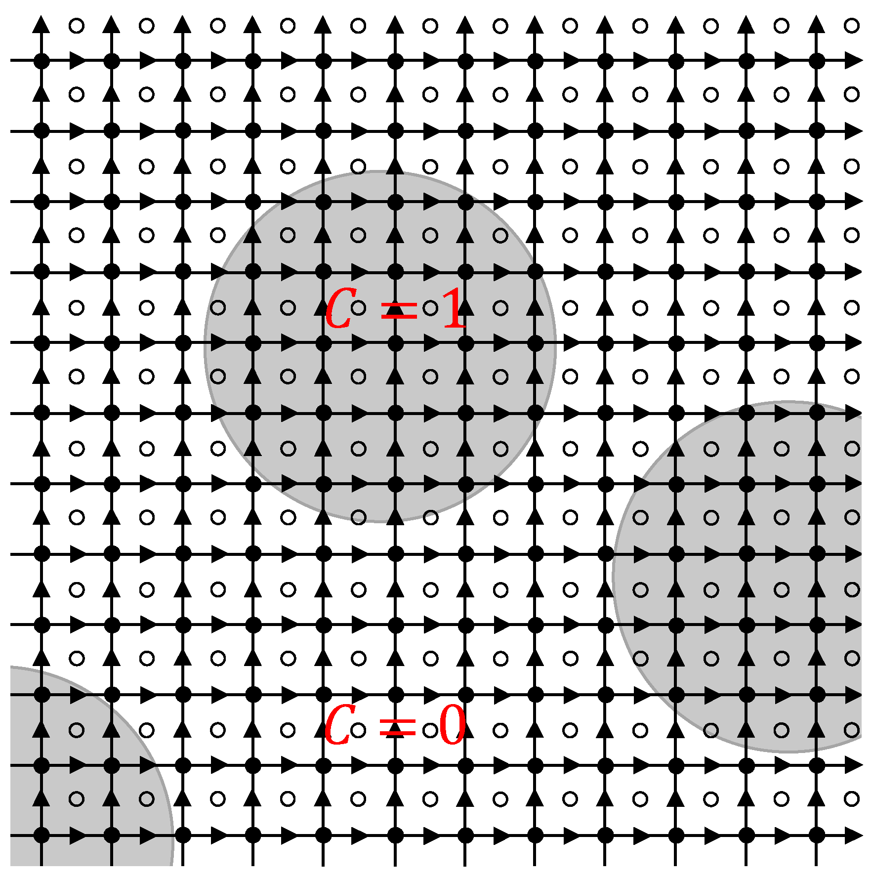
2.1. Viscous Penalty Method

The motion equations of incompressible anisothermal two-phase flows, involving a carrier fluid and a solid particle phase, are based on one-fluid model [20,21], as explained in [9,22]. They are given by:
· u = 0
ρ u t + u · u = p + ρ g + · μ ( u + t u ) + F m
ρ C v T t + u · T = · k f T
where F m is a source term, u is the velocity, p the pressure, T the temperature, t the time, g the gravity vector, ρ , μ , C v and k f respectively the density, the viscosity, the specific heat and the thermal conductivity of the equivalent fluid. Indeed, VPM belongs to the class of fictitious domain methods [23,24], where a fixed mesh for the whole domain (fluid+particles) is used to solve the dynamic of both phases (see Figure 1). Therefore, “equivalent fluid” has the fluid or solid thermophysical properties in the Eulerian cell fully fluid or solid respectively, and is a mix of both in the Eulerian mesh containing the fluid/particle interface. In that sens, specific arithmetic ρ = C ρ s + ( 1 C ) ρ f , C v = C C v s + ( 1 C ) C v f , harmonic μ = μ s μ f C μ f + ( 1 C ) μ s , k f = k f s k f f C k f f + ( 1 C ) k f s laws are used to define them according to a phase function C [22] (the quantities with the subscript s, f refers to those in the solid, fluid respectively). As for the phase function C (also called Color function), it is directly obtained by projecting the shape of the particles on the Eulerian mesh [9,19] (As illustrated in Figure 1). Indeed, at each time iteration, this projection is conducted after the particles positions are updated by solving d x i d t = V i , where V i is the velocity of the i th particle deduced from the Eulerian velocities inside the particle ( x i being its position). This procedure is called VOF-Lag approach in contrast with the classical VOF method [25] where the equation C t + u · C = 0 is solved to update the color function C.
The solid behavior in the zones occupied by the particles (where C = 1 ), is ensured by imposing large values of viscosity in the Eulerian cells inside the particles. Indeed, the strain tensor in (2) tends toward 0 when μ + and based on the equivalence [9] P Ω i , u + T u = 0 V ( P ) = V i + O i P ω i a solid behaviour is, in this way, imposed in the zones inside the particles. Moreover, a specific model [26], based on a decomposition of the viscous stress tensor is implemented to implicitly impose not only the solid behavior (via the viscosity penalization) in the particles but also the coupling between fluid and solid motion.
To satisfy the fluid and solid constraints along with the velocity and pressure coupling, an augmented Lagrangian method is applied to (1), (2) as follows (Algorithm 1) [9]:
Algorithm 1: Augmented Lagrangian (AL) method [27]
  • for each iteration n do
  •      u , 0 = u n and p , 0 = p n
  •      m = 0
  •     while  | | · u , m | | > ϵ A L  do
  •          m = m + 1
  •         solve: ρ u , m u , 0 Δ t + u , m 1 · u , m ( r · u , m ) = p , m 1 + ρ g + · [ μ ( u , m + T u , m ) ]
  •          p , m = p , m 1 r · u , m
  •     end while
  • end for
The mass, momentum and energy equations are discretized using an implicit finite volumes on structured staggered meshes (see Figure 1). The time derivative is approximated with a first order Euler scheme while the inertial, viscous and augmented Lagrangian terms are discretized with second-order centered schemes. All fluxes are written at time ( n + 1 ) Δ t , except the non-linear inertial term that is linearized with a second order Adams-Bashforth scheme as follows
u · u 2 u n u n 1 · u n + 1
The obtained linear system is solved with a BiCGSTAB II iterative solver [28], preconditioned under a Modified and Incomplete LU approach [29] to speed-up the convergence of the solver. All the code is working on massively parallel computers by using MPI [9].
Note that the particles in this work are motionless. Numerically, their velocity is set to zero by imposing the velocity of the Eulerian cells near their centroids to zero by means of a linear term, 10 40 u , added to the Equation (2), and the VPM propagates the zero velocity in the whole solid medium. The particles temperature T s being also constant, they are however imposed in the whole solid medium by means of a linear term, 10 40 ( T T s ) , added to the Equation (3).

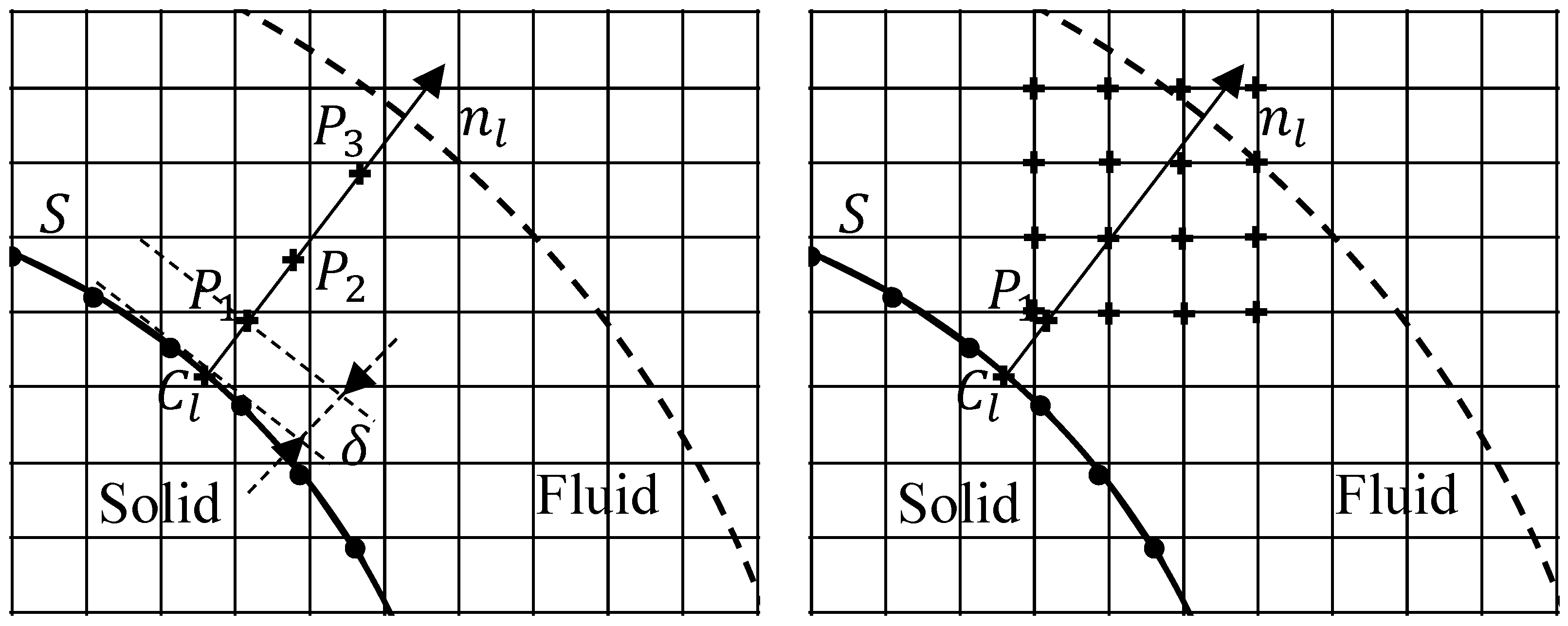
2.2. Heat Transfer Rate Computation

The goal of this work is to extract from the temperature field, solution of the energy Equation (3), the Nusselt number given by:
N u = H p d k f
where d is the particle diameter and H p is the heat transfer rate given by:
H p = Q p T s T f π d 2
Here, T s and T f are the temperatures of the particle and the surrounding fluid respectively, and Q p is the heat flux across the particle surface S. It is given by:
Q p = S k f T · n d S
The computation of the heat flux consists in discretizing S on a set of N elements called Lagrangian mesh (linear segments in 2D and triangles in 3D, see Figure 2), such that:
Q p l N k f T l · n l Δ S l
where the ongoing normal to the lth element n l and its area Δ S l are deduced from its nodes coordinates. However, the temperature T being solved on the Eulerian mesh, the temperature gradient T l is not known at the lth element center C l . To deal with this problem, we have implemented the same approach that the one we have used to obtain the stress tensor σ ¯ ¯ l components on the Lagrangian mesh in the hydrodynamic force computation F l N σ ¯ ¯ l · n l Δ S l . This was detailed in [19]. In this previous work, we have observed that the velocity and the pressure values were inaccurate in the cells containing the interface. Therefore, we had to extrapolate the stress tensor from the area far from the particle to the particle surface. After a numerical study of all the extrapolation parameters, we have reached the conclusion that the third-order Lagrange extrapolation (whose notations are illustrated in Figure 2) is the best compromise between accuracy and computational cost [19]. Similarly, as for force coefficients, we have the temperature gradient at the center of each Lagrangian mesh element as follows:
T ( C l ) = i = 1 3 T ( P i ) L i ( C l ) , where L i ( C l ) = j i 3 | C l P j | | P i P j |
Given that the temperature gradient is computed on the Eulerian mesh and that the extrapolation points P 1 , P 2 and P 3 are constructed in the normal direction to the particle surface (see Figure 2), the temperature gradient at these points are not known. Once again, we relayed on the work [19] to interpolate the temperature gradient from the Eulerian mesh to the extrapolation points P k ( k = 1 , 2 , 3 ) using the third-order Taylor interpolation:
f ( P k ) = f ( E ) + f x i ( E ) ( ( C l ) i E i ) + 1 2 2 f x i 2 ( E ) ( ( C l ) i E i ) 2 + 2 f x i x j ( E ) ( ( C l ) i E i ) ( ( C l ) j E j ) + O ( | | C l E | | 3 )
where E is the nearest Eulerian point to P k .
Another pertinent value to consider when studying the distribution of heat transfers on the surface of the particle, is the local Nusselt number given in the spherical system (see Figure 3) by:
N u l o c ( θ ) = T · n d T s T f
where for each Lagrangian mesh element center ( C l = ( x , y , z ) ), the azimuthal angle θ , and the polar angle β are given by:
θ = ( π arctan 2 ( y 2 + z 2 , x ) ) 180 π , β = arctan 2 ( z , y ) 180 π

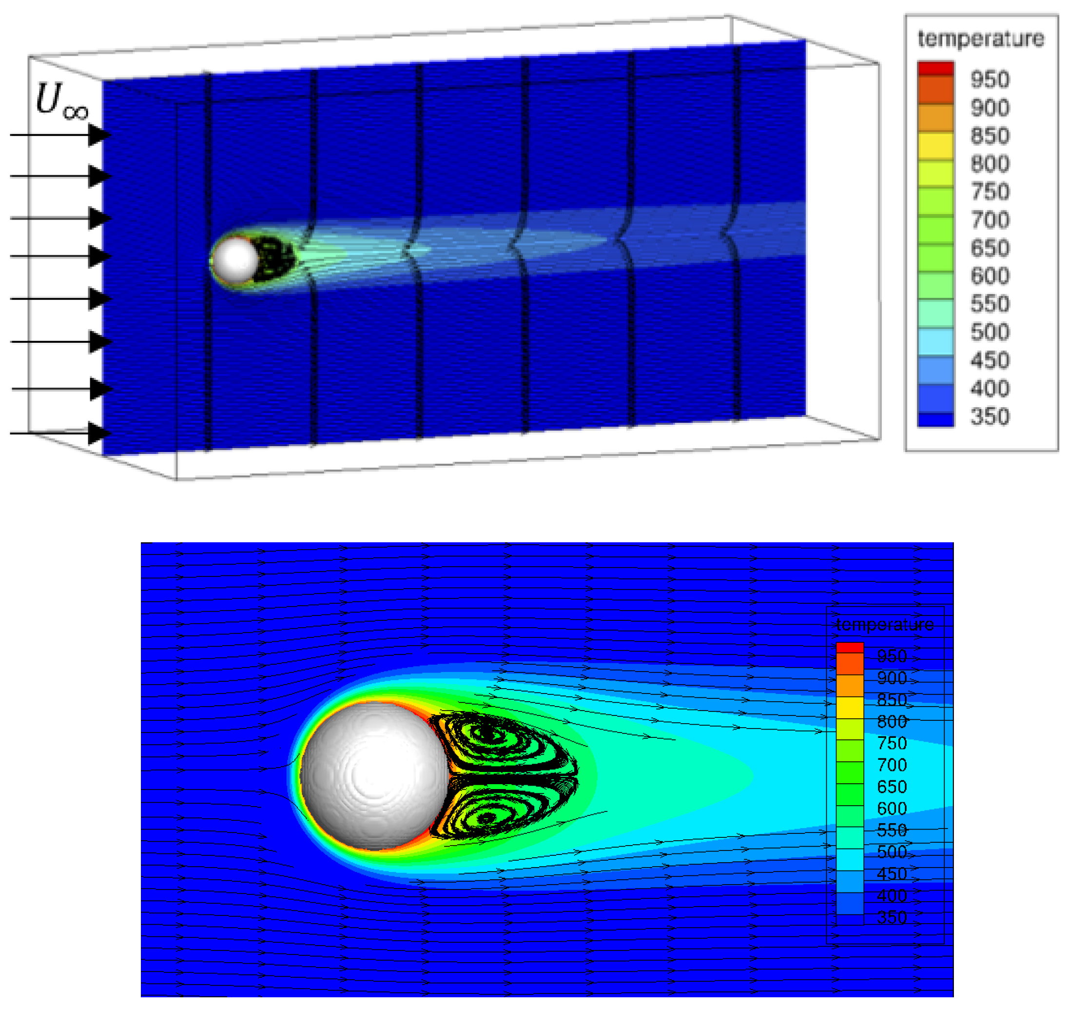
3. Convective Heat Transfer Forced by a Uniform Flow around a Stationary Sphere

The first case considered to validate heat transfer computation is the convection forced by a uniform flow past a hot sphere, illustrated in Figure 4. The computational domain lengths are L x = 16 d and L y = L z = 8 d . The Eulerian mesh refinement is constant in a box of extension 2 d , 3 d , 3 d ; 6 d , 5 d , 5 d centered around the particle position. Outside this box, the Eulerian mesh is exponentially coarsen from the box to the boundaries of the simulation domain. This case was previously used to validate the drag force computation [19]. In the simulations carried out for this case as well as for all the cases studied in this work, we have imposed that the hydrodynamic boundary layer contains five Eulerian cells. Therefore, in the box surrounding the particle, the minimum cell size is Δ x = d 5 R e . This mesh refinement ensures that the hydrodynamic boundary layer contains a sufficient number of extrapolation points to be accurate on force calculations at the particle surface. We have also chosen a Prandtl number P r = 0.72 , which means that the thermal boundary layer is larger than the hydrodynamic boundary layer. In this way, we ensure that enough extrapolation points are available in the thermal boundary layer as well (see Figure 2). The time step is given by Δ t = 0.5 min Δ x U , Δ x 2 k f / C v .

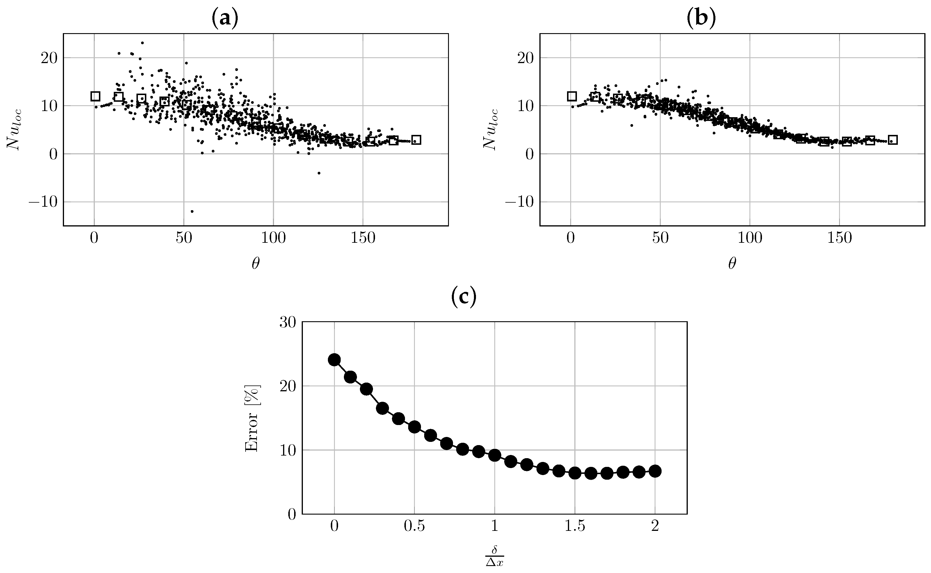
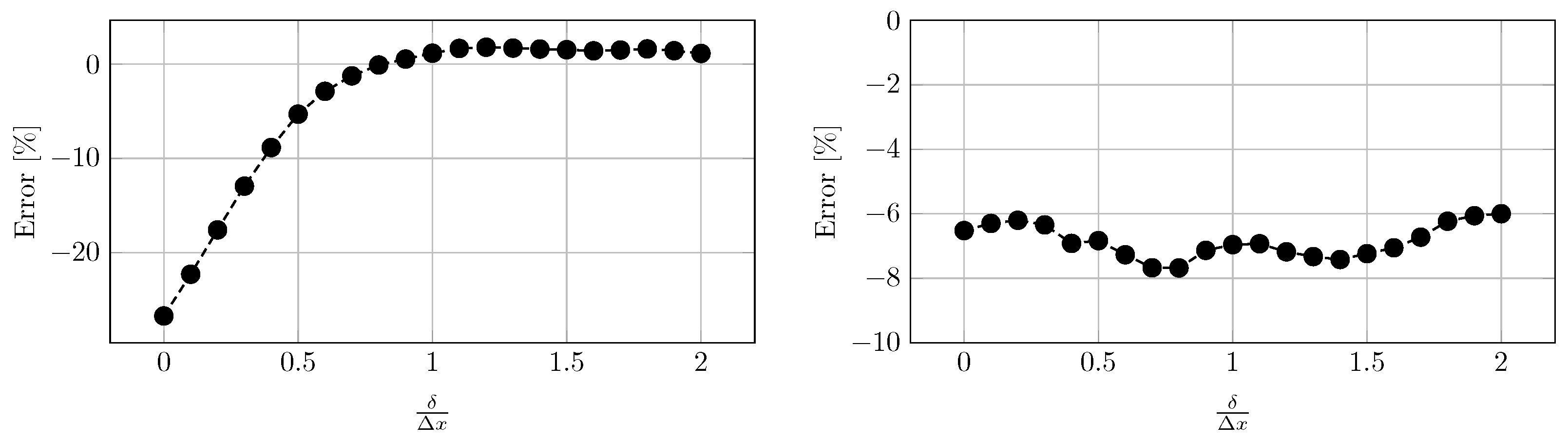
3.1. Effect of the Extrapolation Distance ( δ )

One of the extrapolation parameters studied in the hydrodynamic force computation work [19] was the distance δ between the Lagrangian mesh and the first extrapolation point P 1 (see Figure 2). Indeed, during that study [19], inaccurate pressure and velocity values were observed in the cells cut by the interface, therefore we had to extrapolate the stress tensor from the fluid area far from the particle to the surface. As illustrated in (Figure 5 left), the accurate drag force is reached at δ = Δ x .
The temperature being a function of the velocity (Equation (3)), inaccurate values of the temperature gradient values are also expected in the Eulerian cells containing the interface. Thus, we have conducted the same study for the Nusselt number computation to locate the extrapolation area. But unlike the drag force (Figure 5 left), the Nusselt number computation does not seem to depend on the distance δ (Figure 5 right). Facing this unexpected result, we have compared the distribution of the local Nusselt number to Massol [10] results at R e = 100 where the flow is symmetric with respect to its direction, as illustrated in (Figure 4 right). The local Nusselt number computed for δ = 0 does not reflect the flow symmetry as illustrated in (Figure 6a), and the error between our result ( N u l o c ) and Massol’s ( N u l o c M a s s o l ) given by i = 1 N | N u l o c i N u l o c M a s s o l i | i = 1 N | N u l o c M a s s o l i | is about 25 % . This error decreases as the distance δ increases until being lower than 10 % for δ 1 (Figure 6c). It is worth noting that for this distance, the local Nusselt number distribution more accurately reflects the expected symmetry of the flow as it satisfies almost the same distribution for all the polar angle ( β ) plans (Figure 6b). So, as for the hydrodynamic force computation [19] and in the rest of this work, the extrapolation distance will always be δ = 1 .

3.2. Result on the Nusselt Coefficient

The numerical parameters of the heat transfer on the particle surface being set up, the global Nusselt number for a uniform flow past a hot sphere at different Reynolds number ( R e = 10 , 20 , 40 , 60 , 80 , 100 , 150 , 200 , 250 , 290 ) is computed using the presented method and compared to the following correlations:
  • Ranz and Marshall [31]:
    N u = 2 . + 0.6 R e 0.5 P r 1 3
  • Feng and Michaelides [32]:
    N u = 0.992 + R e P r 1 3 + 0.1 R e 2 3 P r 1 3
  • Whitaker [33]:
    N u = 2 . + 0.4 R e 0.5 + 0.06 R e 2 3 P r 0.4
Figure 7 provides the comparisons of our results to literature references. It can be observed that our simulated Nusselt values belong to the same value ensemble as literature works for all considered Reynolds numbers. If we go into more detail, the Nusselt numbers simulated with VPM show a better agreement with Feng and Michaelides and Whitaker correlations than with Ranz and Marshall.

4. Face-Centered Cubic Periodic Arrangement of Spheres

The second case studied in this work is a uniform flow past a Face-Centered Cubic (FCC) array of hot spheres which consists in a cube where three spheres are placed on the faces centers, and one sphere is located on the vertices with periodic boundary conditions, as illustrated in Figure 8. The domain length L is deduced from the solid volume fraction α d : L = 2 3 π α d 1 / 3 d . Given a Reynolds number R e = ρ d u d μ , a desired mean fluid velocity u f = u d is enforced via the source term
F m = ρ u f u d Δ t + i N p F i D V f
inserted in the momentum conservation Equation (2). F i D is the drag force computed over the ith particle using the method described in [19] and V f is the volume occupied by the fluid. F m is thus adjusted until the stationary state is reached when u f = u d . As for the uniform flow past an isolated sphere, the grid resolution is fixed by imposing five Cartesian cells in the boundary layer: Δ x = d 5 R e , and the time step is given by Δ t = 0.5 min Δ x U , Δ x 2 k f / C v .
This case was previously used to validate the hydrodynamic force computation [19]. In that previous work [19], the hydrodynamic force was computed when the steady-state of the flow was reached. This steady state obtained in an isothermal context is used in the present simulations as the initial condition for the momentum equation ‘Equation (2)’. In addition, the initial temperature conditions for the energy equation ‘Equation (3)’ are T s = 1 , T f = 0.5 , respectively the sphere and the fluid temperature. In this problem, the fluid heats up until its temperature < T > f (averaged on the fluid domain) reaches the sphere temperature (see Figure 9 left). In the meantime and after an initialization time of the temperature gradient around the spheres, a balance is reached between the heat flux and the difference between the fluid and the particle temperature. This results in the apparition of a plateau in the global Nusselt coefficient temporal evolution as illustrated in Figure 9 right. Therefore, the Nusselt number for a uniform flow past a FCC array of spheres is the value at this stabilized state.
Note that the global and local Nusselt coefficients for a uniform flow past an array of N p particles are an average of those computed on each sphere such as:
N u = 1 N p i N p N u i N u l o c = 1 N p i N p ( N u l o c ) i
where N p = 4 for a FCC array.

4.1. Flow Analysis

Using the local Nusselt coefficient distribution presented in Figure 10, two regimes can be observed, i.e., attached (illustrated in Figure 8 left) and separated (Figure 8 right) flows, that govern the uniform flow past a FCC array of spheres, depending on the Reynolds number and the solid volume fraction α d :

4.1.1. Attached Flows

For low Reynolds numbers, the local Nusselt number is having the same behavior as for an isolated sphere (see Figure 10 left). The increase of its value is due to the presence of the other spheres (blocking effect) that speed up the flow and therefore flatten the boundary layer which increases the temperature gradient. We can also observe that the presence of surrounding particles breaks the symmetry of the flow. Indeed, (Figure 10 left) shows two distinct distributions of the local Nusselt number for two different plans ( β = 0 ) and ( β = 45 ) , and these results are in good agreement with Massol body fitted simulations [10].

4.1.2. Separated Flows Downstream of the Spheres

By increasing the Reynolds number, a separated flow appears downstream of the spheres together with a fountain effect upstream of the spheres (see Figure 8 right). These phenomena can be observed also in the local Nusselt number distribution (Figure 10 right). Indeed, the higher value of the Nusselt number is no more at the upstream stagnation point θ = 0 , due to the fountain effect that induces a low heat flux. With increasing θ , i.e., leaving the fountain zone, the Nusselt number increases as the boundary layer shrinks due to the fluid acceleration in this zone. It then decreases until the separation point, where the fluid temperature is the highest. Finally, the Nusselt increases again in the recirculating zone behind the sphere.

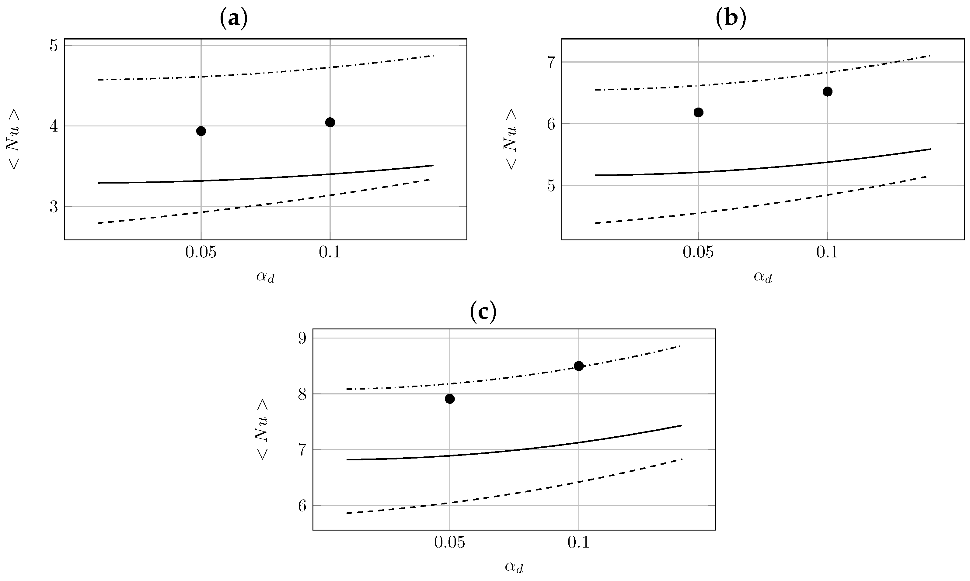
4.2. Global Nusselt Coefficient

The Nusselt number of a uniform flow past an FCC array of spheres normalized by the isolated sphere Nusselt number (given by Ranz and Marshall [31]) N u s = 2 . + 0.6 R e 0.5 P r 1 3 , noted N u N u s , is compared to existing literature results. This comparison, illustrated in Figure 11, shows a nice match with Massol [10] results at different Reynolds number and for a large range of solid volume fraction ( 0.05 α d 0.6 ) . A good agreement is also observed with Gun [14] correlation for low solid volume fractions ( α d 0.15 ) , which means that for this range of α d , the FCC configuration is a good approximation of a uniform flow past a random assembly of spheres.
This study shows the strong dependence of the global Nusselt number to the solid volume fraction and Reynolds number. Indeed, increasing the solid volume fraction increases the blocking effect which reduces the thickness of the thermal boundary layer and at the same time, increases the temperature gradient and consequently the Nusselt number. This effect accentuate significantly with the solid volume fraction. Indeed, Nusselt number for a sphere in FCC configuration can be five times higher than for an isolated sphere for high particle concentrations. Moreover, the Nusselt number of a sphere in an FFC arrangement seems to diverge from the Gunn correlation [14] for large solid volume fraction. Therefore, the FCC configuration is not a suitable approximation for a uniform flow past a random assembly of spheres at dense regime.

5. Finite Size Random Arrangement of Spheres

In order to assess the ability of the presented method to deal with more complex particulate flows, the last case studied in this work is a uniform flow past a random assembly of fixed hot spheres of diameter d (illustrated in Figure 12). The computational domain lengths are L x = 9 d and L y = L z = 5 d . Given a solid volume fraction α d , the particles are randomly distributed in the sub-domain 2 d , 0 , 0 ; 7 d , 5 d , 5 d . The assembly of spheres is filled by generating one sphere after an other. The position of the new sphere is randomly generated and a very straightforward overlap test is conducted with the already generated spheres. If no overlap is detected, the new particle is added to the assembly, otherwise, the sphere is rejected and a new sphere is generated in the same manner. The procedure is repeated until the desired solid volume fraction is reached. Furthermore, a cold fluid flows through the channel in the x-direction (streamwise), by imposing at the inlet a temperature T and a velocity U x deduced from Reynolds number R e = U d ν . Periodic boundary conditions are imposed in crosswise directions. The N p spheres are maintained at a constant temperature T s , the number of spheres is deduced from the solid volume fraction by N p = 6 π L y d 3 α d . As for the two previous cases, the grid resolution and the time step are given by: Δ x = d 5 R e , Δ t = 0.5 min Δ x U , Δ x 2 k f / C v .
A fixed bed Nusselt number is considered here. It is defined as an average of individual particle Nusselt numbers:
N u = 1 N p i N p ( Q p ) i T s ( T f ) i π d 2
where ( Q p ) i is the i th sphere heat flux given by ‘Equation (8)’. Estimating the local average temperature of the fluid ( T f ) i is not straightforward. As suggested by Deen et al. [12], a good estimate is given by:
( T f ) i = ( 1 C ) T g i ( r ) ( 1 C ) g i ( r )
where T and C are the temperature field and color function respectively, and g i ( r ) is the filter that covers the fluid volume in a 4 d length box containing the i th sphere, both having the same center. It is given by:
g i ( r ) = exp 2 r d , 0 < r < 2 d
Simulations of uniform flow past a random assembly of hot spheres were performed for low solid volume fractions α d = 0.05 , 0.1 at different Reynolds numbers R e = 10 , 50 , 100 . Their results are compared to the following correlations:
  • Gun [14]:
    N u = 7 10 1 α d + 5 1 α d 2 1 + 0.7 R e 0.2 P r 1 3 + 1.33 2.4 1 α d + 1.2 1 α d 2 R e 0.7 P r 1 3
  • Deen et al. [16]:
    N u = 7 10 1 α d + 5 1 α d 2 1 + 0.17 R e 0.2 P r 1 3 + 1.33 2.31 1 α d + 1.16 1 α d 2 R e 0.7 P r 1 3
  • Sun et al. [17]:
    N u = 0.46 + 1.77 1 α d + 0.69 1 α d 2 1 α d 3 + 1.37 2.4 1 α d + 1.2 1 α d 2 R e 0.7 P r 1 3
Figure 13 shows that our results are in the same range of values than the results given in the literature, which is very encouraging as first results of real particle flow arrangements.

6. Conclusions

In the framework of a finite-size particle approach, an accurate procedure for the calculation of heat transfer coefficients for motions around fixed particles has been proposed based on third order Lagrange extrapolation coupled to third order Taylor interpolation methods. This method is an extension of the techniques proposed for hydrodynamic force estimates published in [19]. The procedure allowing the estimate of heat transfer coefficients at a particle surface has been validated with success on fixed isolated spheres, FCC and random arrangements of spheres. Comparisons have been presented to reference Nusselt correlations of the literature.
Future works will be devoted to applying our heat transfer calculation method to arrangements of ellipsoidal particles and extracting correlation laws for these configurations. Moreover, a more extensive study of heat transfer in a fluidized bed is now possible.

Author Contributions

Conceptualization, M.-A.C., S.V. and J.-L.E.; methodology, M.-A.C. and S.V.; software, M.-A.C. and S.V.; validation, M.-A.C.; formal analysis, M.-A.C.; investigation, M.-A.C.; resources, M.-A.C.; data curation, M.-A.C.; writing—original draft preparation, M.-A.C. and S.V.; writing—review and editing, M.-A.C. and S.V.; visualization, M.-A.C.; supervision, S.V. and J.-L.E.; project administration, S.V.; funding acquisition, S.V. and J.-L.E. All authors have read and agreed to the published version of the manuscript.

Funding

This research was funded by ANR grant number ANR-11-BS09-0004.

Institutional Review Board Statement

Not applicable.

Informed Consent Statement

Not applicable.

Acknowledgments

The authors gratefully acknowledge support from CINES (National Computing Center for Higher Education), IDRIS (Institut du développement et des ressources en informatique scientifique) and CCRT (National Computing Center of CEA) under project number A0092B06115.

Conflicts of Interest

The authors declare no conflict of interest.

References

  1. Bagheri, G.; Bonadonna, C.; Manzella, I.; Vonlanthen, P. On the characterization of size and shape of irregular particles. Powder Technol. 2015, 270, 141–153. [Google Scholar] [CrossRef]
  2. Dartevelle, S. From Model Conception to Verification and Validation, a Global Approach to Multiphase Navier-Stoke Models with an Emphasis on Volcanic Explosive Phenomenology. Technical Report LA-14346, 948564; 2007. Available online: https://permalink.lanl.gov/object/tr?what=info:lanl-repo/lareport/LA-14346 (accessed on 9 September 2021).
  3. Adanez, J.; Abad, A.; Garcia-Labiano, F.; Gayan, P.; de Diego, L.F. Progress in Chemical-Looping Combustion and Reforming technologies. Prog. Energy Combust. Sci. 2012, 38, 215–282. [Google Scholar] [CrossRef] [Green Version]
  4. Lyngfelt, A.; Leckner, B.; Mattisson, T. A fuidized-bed combustion process with inherent CO2 separation; application of chemical-looping combustion. Chem. Eng. Sci. 2001, 56, 3101–3113. [Google Scholar] [CrossRef]
  5. Mattisson, T.; Keller, M.; Linderholm, C.; Moldenhauer, P.; Rydan, M.; Leion, H.; Lyngfelt, A. Chemical-looping technologies using circulating fluidized bed systems: Status of development. Fuel Process. Technol. 2018, 172, 1–12. [Google Scholar] [CrossRef] [Green Version]
  6. Acrivos, A.; Hinch, E.J.; Jeffrey, D.J. Heat transfer to a slowly moving fluid from a dilute fixed bed of heated spheres. J. Fluid Mech. 1980, 101, 403–421. [Google Scholar] [CrossRef] [Green Version]
  7. Pfeffer, R.; Happel, J. An analytical study of heat and mass transfer in multiparticle systems at low Reynolds numbers. AIChE J. 1964, 10, 605–611. [Google Scholar] [CrossRef]
  8. Wakao, N.; Kaguei, S. Heat and Mass Transfer in Packed Beds Volume 1; Gordon and Breach Science Publishers Inc.: New York, NY, USA, 1983. [Google Scholar]
  9. Vincent, S.; de Motta, J.C.B.; Sarthou, A.; Estivalezes, J.L.; Simonin, O.; Climent, E. A Lagrangian VOF tensorial penalty method for the DNS of resolved particle-laden flows. J. Compuat. Phys. 2014, 256, 582–614. [Google Scholar] [CrossRef] [Green Version]
  10. Massol, A. Simulations Numériques d’écoulements à Travers des réseaux Fixes de Spheres Monodisperses et Bidisperses, Pour des Nombres de Reynolds Modérés. Ph.D. Thesis, Institut National Polytechnique de Toulouse, Toulouse, France, 2004. Available online: https://www.researchgate.net/publication/242075914_Adaptive_Augmented_Lagrangian_techniques_for_simulating_unsteady_multiphase_flows (accessed on 9 September 2021).
  11. Schönfeld, T.; Rudgyard, M. Steady and Unsteady Flow Simulations Using the Hybrid Flow Solver AVBP. AIAA J. 1999, 37, 1378–1385. [Google Scholar] [CrossRef]
  12. Deen, N.G.; Kriebitzsch, S.H.; van der Hoef, M.A.; Kuipers, J. Direct numerical simulation of flow and heat transfer in dense fluid–particle systems. Chem. Eng. Sci. 2012, 81, 329–344. [Google Scholar] [CrossRef]
  13. Tavassoli, H.; Kriebitzsch, S.; van der Hoef, M.; Peters, E.; Kuipers, J. Direct numerical simulation of particulate flow with heat transfer. Int. J. Multiph. Flow 2013, 57, 29–37. [Google Scholar] [CrossRef]
  14. Gunn, D. Transfer of heat or mass to particles in fixed and fluidized beds. Int. J. Heat Mass Transf. 1978, 21, 467–476. [Google Scholar] [CrossRef]
  15. Tenneti, S.; Sun, B.; Garg, R.; Subramaniam, S. Role of fluid heating in dense gas-solid flow as revealed by particle-resolved direct numerical simulation. Int. J. Heat Mass Transf. 2013, 58, 471–479. [Google Scholar] [CrossRef]
  16. Deen, N.G.; Peters, E.A.J.F.; Padding, J.T.; Kuipers, J.A.M. Review of direct numerical simulation of fluid-particle mass, momentum and heat transfer in dense gas-solid flows. Chem. Eng. Sci. 2014, 116, 710–724. [Google Scholar] [CrossRef]
  17. Sun, B.; Tenneti, S.; Subramaniam, S. Modeling average gas–solid heat transfer using particle-resolved direct numerical simulation. Int. J. Heat Mass Transf. 2015, 86, 898–913. [Google Scholar] [CrossRef] [Green Version]
  18. Thiam, E.I.; Masi, E.; Climent, E.; Simonin, O.; Vincent, S. Particle-resolved numerical simulations of the gas–solid heat transfer in arrays of random motionless particles. Acta Mech. 2019, 230, 541–567. [Google Scholar] [CrossRef] [Green Version]
  19. Chadil, M.A.; Vincent, S.; Estivalèzes, J.L. Accurate estimate of drag forces using particle-resolved direct numerical simulations. Acta Mech. 2018, 230, 569–595. [Google Scholar] [CrossRef] [Green Version]
  20. Kataoka, I. Local instant formulation of two-phase flow. Int. J. Multiph. Flow 1986, 12, 745–758. [Google Scholar] [CrossRef]
  21. Kataoka, I.; Ishii, M.; Serizawa, A. Local formulation and measurements of interfacial area concentration in two-phase flow. Int. J. Multiph. Flow 1986, 12, 505–529. [Google Scholar] [CrossRef]
  22. Chadil, M.A.; Vincent, S.; Estivalezes, J.L. Improvement of the Viscous Penalty Method for Particle-Resolved Simulations. Open J. Fluid Dyn. 2019, 09, 168–192. [Google Scholar] [CrossRef] [Green Version]
  23. Glowinski, R.; Pan, T.W.; Hesla, T.I.; Joseph, D.; Périaux, J. A fictitious domain approach to the direct numerical simulation of incompressible viscous flow past moving rigid bodies: application to particulate flow. J. Comput. Phys. 2001, 169, 363–426. [Google Scholar] [CrossRef] [Green Version]
  24. Khadra, K.; Angot, P.; Parneix, S.; Caltagirone, J. Fictitious domain approach for numerical modelling of Navier-Stokes equations. Int. J. Numer. Methods Fluids 2000, 34, 651–684. [Google Scholar] [CrossRef]
  25. Hirt, C.W.; Nichols, B.D. Volume of fluid (VOF) method for the dynamics of free boundaries. J. Comput. Phys. 1981, 39, 201–225. [Google Scholar] [CrossRef]
  26. Caltagirone, J.P.; Vincent, S. Tensorial penalisation method for solving Navier–Stokes equations. Comptes Rendus De L’académie Des Sci. Paris Série IIb 2001, 329, 607–613. [Google Scholar]
  27. Vincent, S.; Larocque, J.; Lubin, P.; Caltagirone, J.P.; Pianet, G.; Climent, E. Adaptive Augmented Lagrangian Techniques for Simulating Unsteady Multiphase Flows. In Proceedings of the 6th International Conference on Multiphase Flow, ICMF 2007, Leipzig, Germany, 9–13 July 2007. [Google Scholar]
  28. Gustafsson, I. On First- and Second-Order Symmetric Factorisation Methods for the Solution of Elliptic Difference Equations; Chalmers University of Technology: Gothenburg, Sweden, 1978. [Google Scholar]
  29. der Vost, H.V. Bi-CGSTAB: A fast and smoothly converging variant of Bi-CG for the solution of non-symmetric systems. SIAM J. Sci. Comput. 1992, 33, 631–644. [Google Scholar] [CrossRef]
  30. Schiller, L.; Naumann, A.Z. Über die grundlegenden Berechnungen bei der Schwerkraftaufbereitung. Ver. Deut. Ing. 1933, 77, 318–320. [Google Scholar]
  31. Ranz, W.E.; Marshall, W.R. Evaporation from drops. Parts I & II. Chem. Eng. Progr. 1952, 48, 141–146. [Google Scholar]
  32. Feng, Z.G.; Michaelides, E.E. A numerical study on the transient heat transfer from a sphere at high Reynolds and Peclet numbers. Int. J. Heat Mass Transf. 2000, 43, 219–229. [Google Scholar] [CrossRef]
  33. Whitaker, S. Forced convection heat transfer correlations for flow in pipes, past flat plates, single cylinders, single spheres, and for flow in packed beds and tube bundles. AIChE J. 1972, 18, 361–371. [Google Scholar] [CrossRef]
Figure 1. Projected phase function C on staggered grids. Pressure in black circles, the velocities as arrows and viscosity in white circles [9].
Fluids 07 00015 g001
Figure 2. Notations for the third order Lagrange extrapolation (left) and the third order Taylor interpolation (right), used in heat flux computations.
Fluids 07 00015 g002
Figure 3. Spherical coordinate system around a particle. The flow direction is represented by the undisturbed velocity U .
Fluids 07 00015 g003
Figure 4. Streamlines and temperature field in a slice for a uniform flow past a sphere at R e = 100 . The bottom figure is a zoom on the particle.
Fluids 07 00015 g004
Figure 5. Drag force relative error to Schiller and Naumann [30] correlation (left) and Nusselt number relative error to Ranz&Marshall [31] correlation (right), as a function of the distance δ at R e = 100 .
Fluids 07 00015 g005
Figure 6. Local Nusselt coefficient for a uniform flow past an isolated sphere at R e = 100 , as function of the azimuthal angle θ , for all points on the particle surface (for all β plans) at (a) δ = 0 and (b) δ = 1 : (.) present work, (□) Massol [10]. (c) is local Nusselt number relative error to Massol’s result [10] as function of the extrapolation distance δ .
Fluids 07 00015 g006
Figure 7. Nusselt coefficient for the uniform flow past a hot sphere at different Reynolds numbers: ( Fluids 07 00015 i001) Ranz and Marshall [31], ( Fluids 07 00015 i002) Feng and Michaelides [32], ( Fluids 07 00015 i003) Whitaker [33], (•) present work.
Fluids 07 00015 g007
Figure 8. Streamlines and temperature field for a steady flow along the x-axis of a Face-Centered Cubic array of spheres at R e = 50 , α d = 0.15 (left), and at R e = 300 , α d = 0.15 (right).
Fluids 07 00015 g008
Figure 9. Left: Time evolution of fluid temperature for a uniform flow past a Face-Centered Cubic array of spheres at R e = 50 and (◇) α d = 0.05 , (△) α d = 0.1 , (□) α d = 0.15 , (♦) α d = 0.3 , (•) α d = 0.4 , (▲) α d = 0.5 , (◯) α d = 0.6 . Right: Time evolution of the averaged Nusselt coefficient for a uniform flow past a Face-Centered Cubic array of spheres at R e = 50 and α d = 0.4 .
Fluids 07 00015 g009
Figure 10. Left: Local nusselt number for a uniform flow past an isolated sphere at R e = 50 (▲) and for a uniform flow past a FCC array of spheres at R e = 50 , α d = 0.15 : β = 0 ((△) Massol [10], (♦) present work ) and β = 45 ((□) Massol [10], (•) present work ). Right: Local Nusselt number for a uniform flow past a FCC array of spheres at R e = 300 , α d = 0.15 : β = 0 (◯), β = 22.5 (△), β = 45 (□).
Fluids 07 00015 g010
Figure 11. Global Nusselt coefficient for a uniform flow past a FCC, normalized by Ranz and Marshall [31] Nusselt coefficient for a uniform flow past an isolated sphere. Evolution as a function of the solid volume fraction α d at Reynolds numbers ( a ) R e = 10 , ( b ) R e = 50 , ( c ) R e = 100 : ( Fluids 07 00015 i001
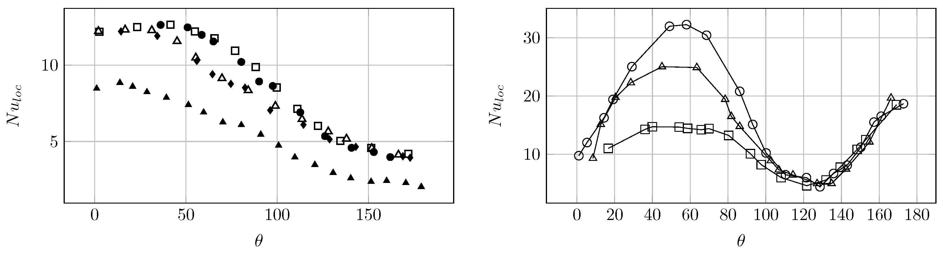
) Gunn [14], (□) Massol [10], (•) present work.
Fluids 07 00015 g011
Figure 12. Streamlines and temperature field of a steady flow along the x-axis of a random array of spheres at R e = 100 and α d = 0.1 .
Fluids 07 00015 g012
Figure 13. Nusselt coefficient for a uniform flow past a random arrangement of hot spheres as a function of the solid volume fraction α d at vatious Reynolds numbers (a) R e = 10 , (b) R e = 50 , (c) R e = 100 : ( Fluids 07 00015 i003) Gunn [14], ( Fluids 07 00015 i001) Deen et al. [16], ( Fluids 07 00015 i002) Sun et al. [17] and (•) present work.
Fluids 07 00015 g013
Publisher’s Note: MDPI stays neutral with regard to jurisdictional claims in published maps and institutional affiliations.

