
Impact of Climate Change on the Hydrological Regime of the Yarkant River Basin, China: An Assessment Using Three SSP Scenarios of CMIP6 GCMs

Abstract
:1. Introduction
2. Materials
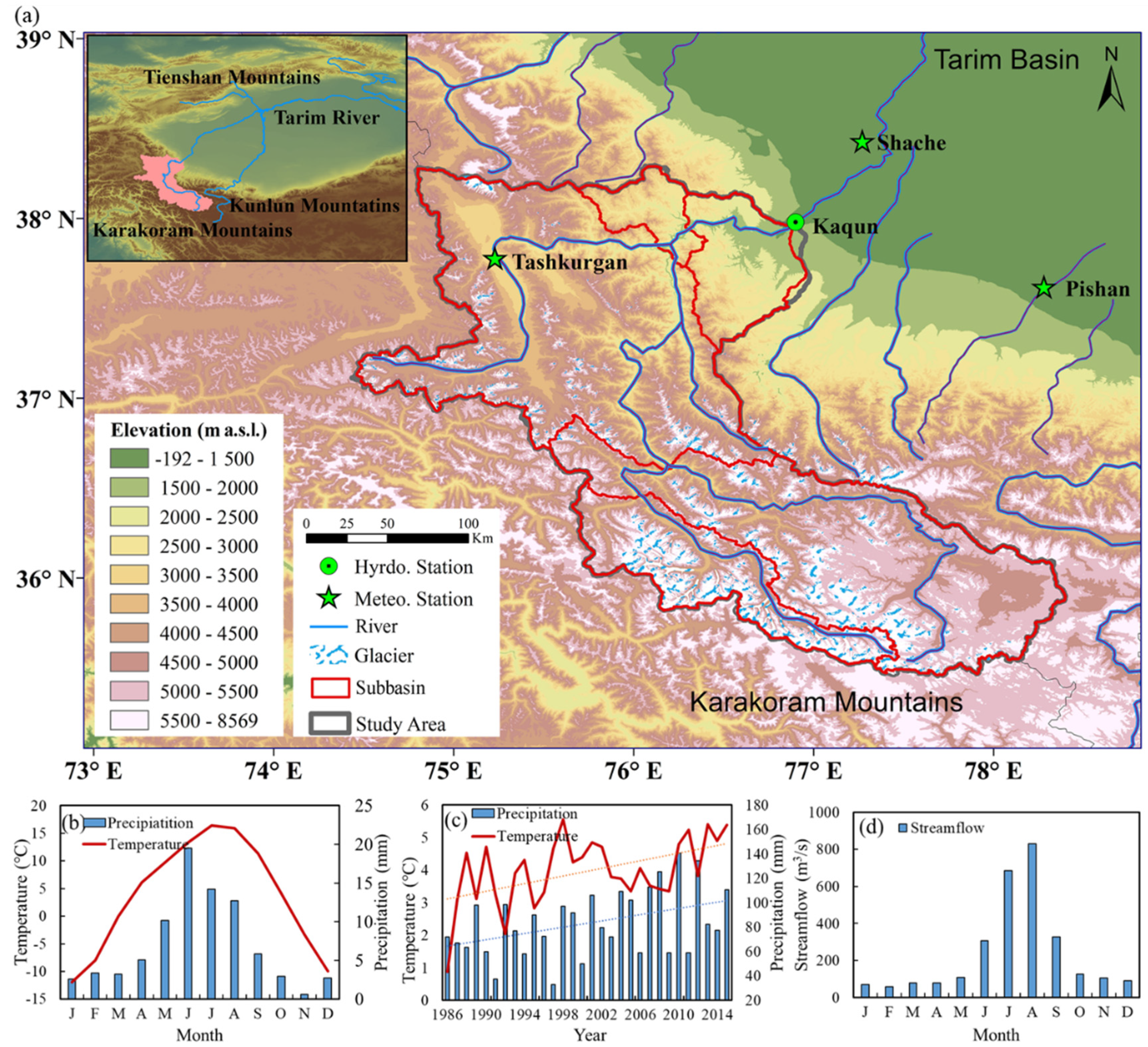
2.1. Study Area
2.2. Datasets
2.3. The Hydrological Model
2.4. Model Performance Evaluation
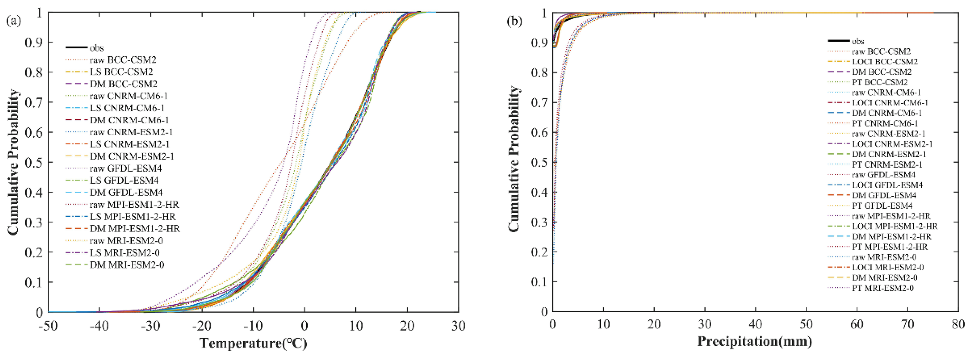
2.5. Bias-Correction Methods and Performance Evaluation
- For air temperature, the performance of corrected air temperature was evaluated using frequency-based and time-series-based metrics compared to observation data. The frequency-based metrics included the mean, median, and 10% and 99% deciles, while the time-series-based metrics included the root mean square error RMSE, R2, and MAE, where:The smaller the root mean square error (RMSE), R2, and mean absolute error (MAE) values, the more reliable the model is in comparison to the observed data.
- For precipitation, the performance of corrected precipitation was evaluated using frequency-based and time-series-based indicators. The frequency-based indicators included the mean, median, standard deviation, wet day frequency, and wet day precipitation intensity, while the time-series-based indicators included the RMSE and MAE.
2.6. Extreme Flows
3. Results
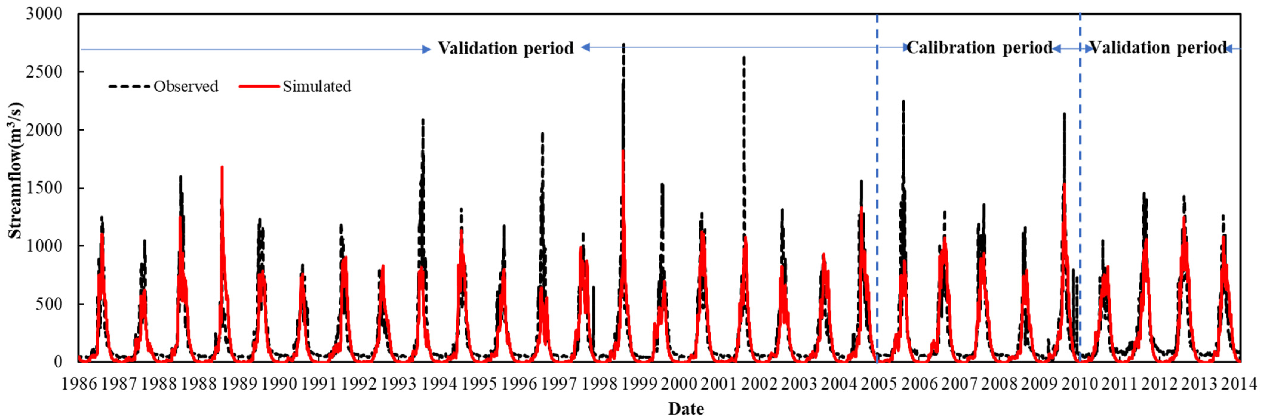
3.1. Model Setup
3.2. Evaluation of Bias Correction Approaches
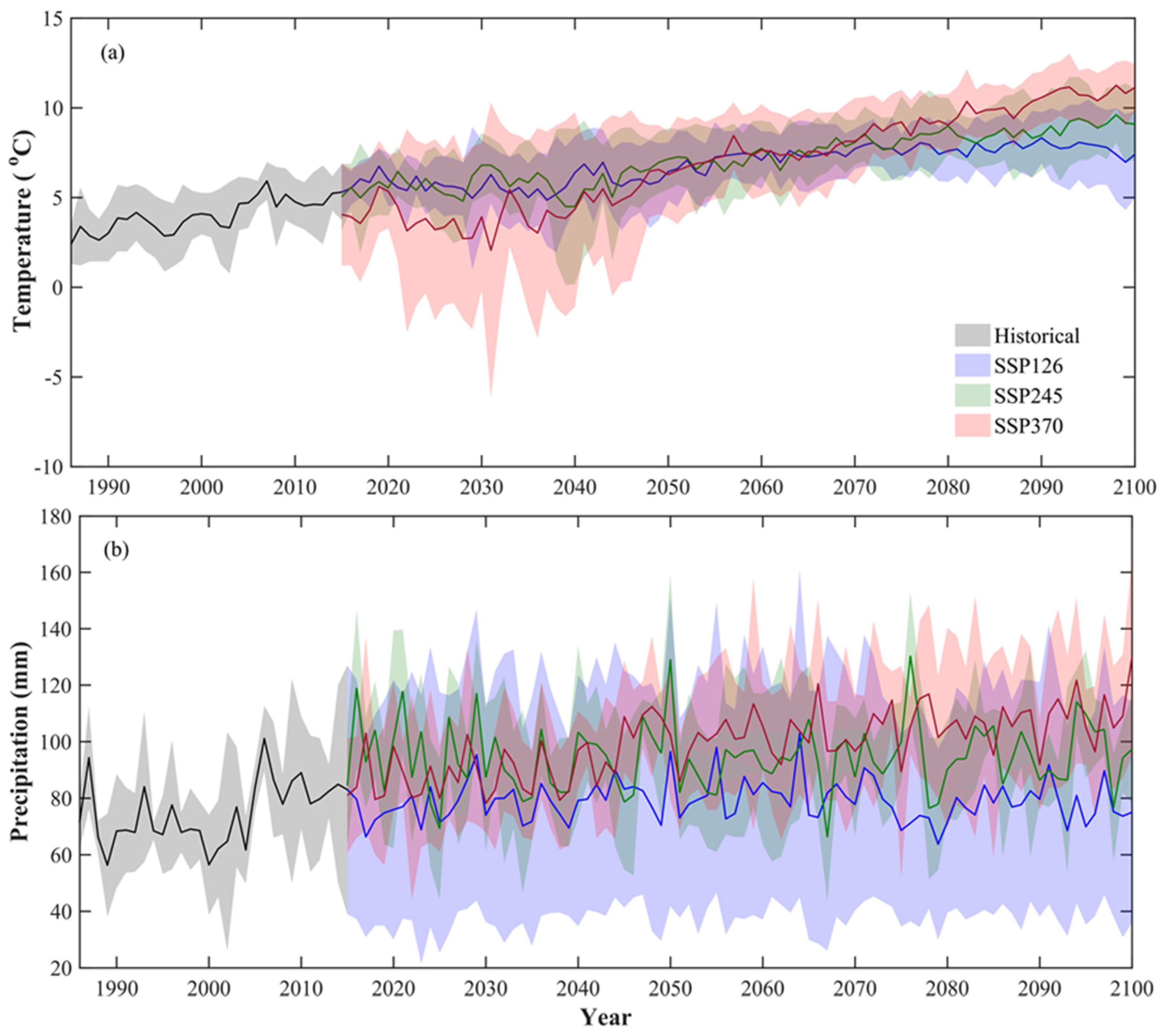
3.3. Climate Projections and Climate Change Analysis
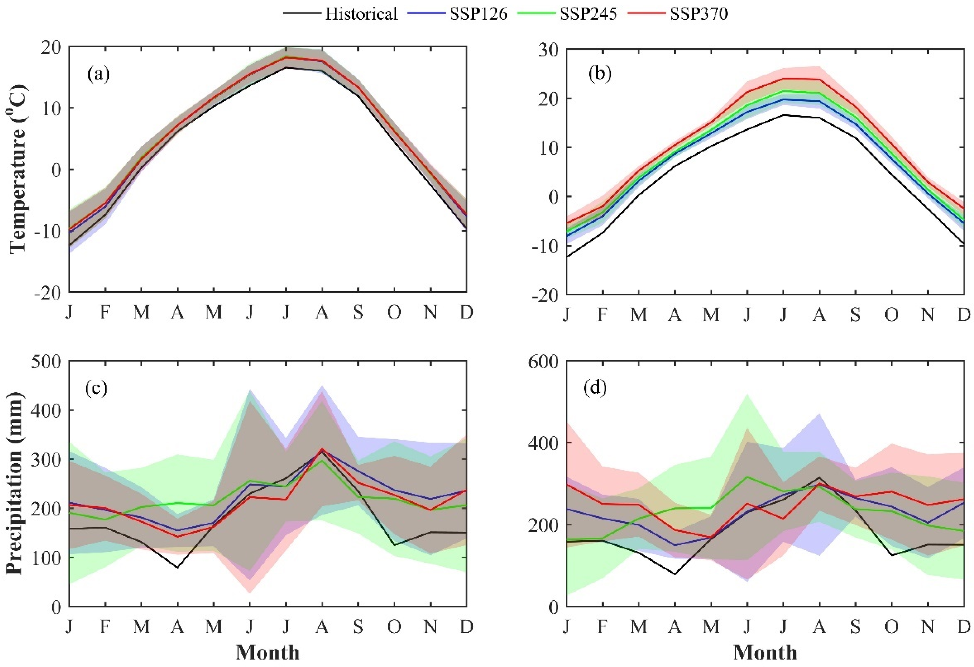
3.3.1. Temperature Projection
3.3.2. Precipitation Projection
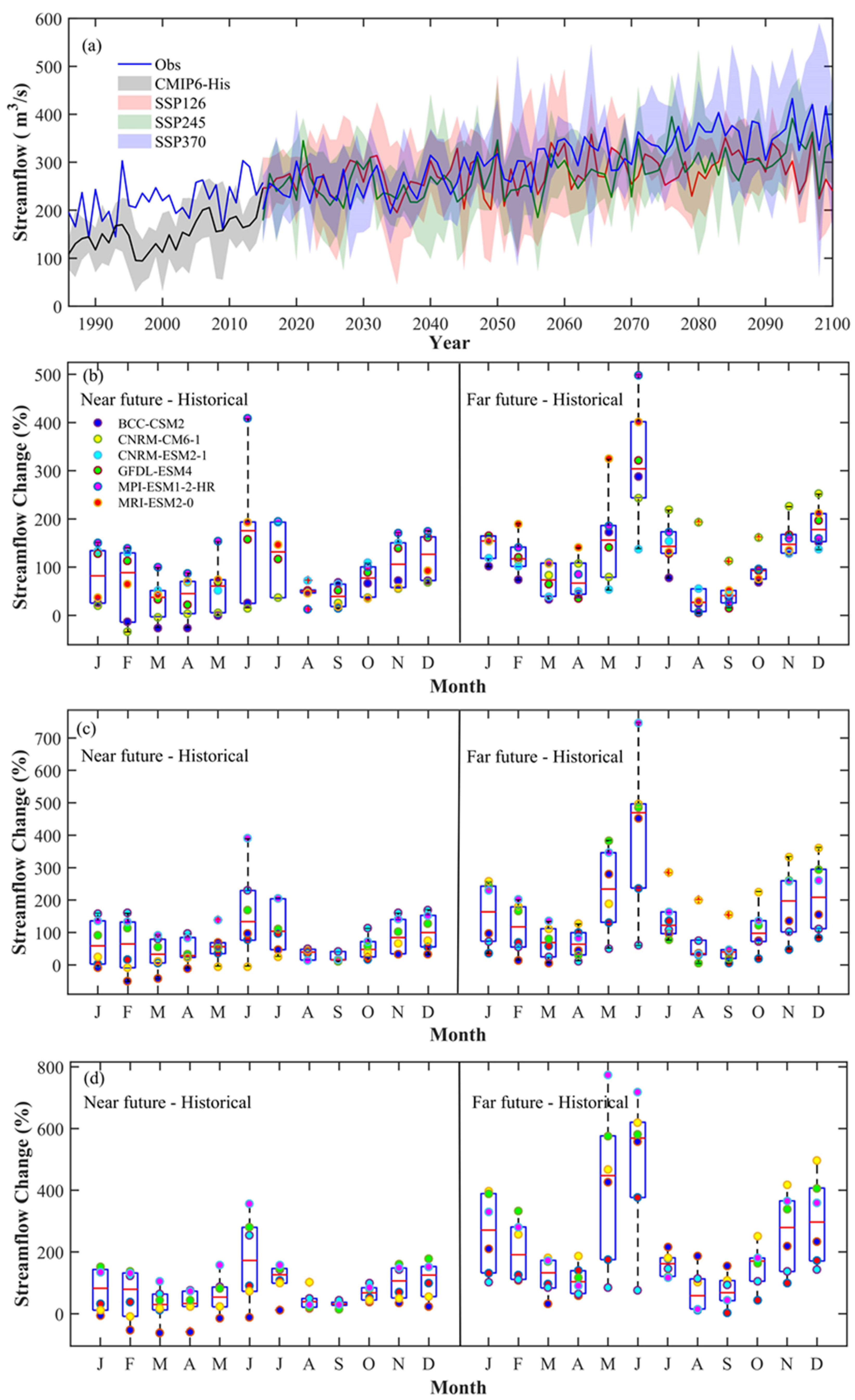
3.4. Streamflow Change Predictions to Changing Climate
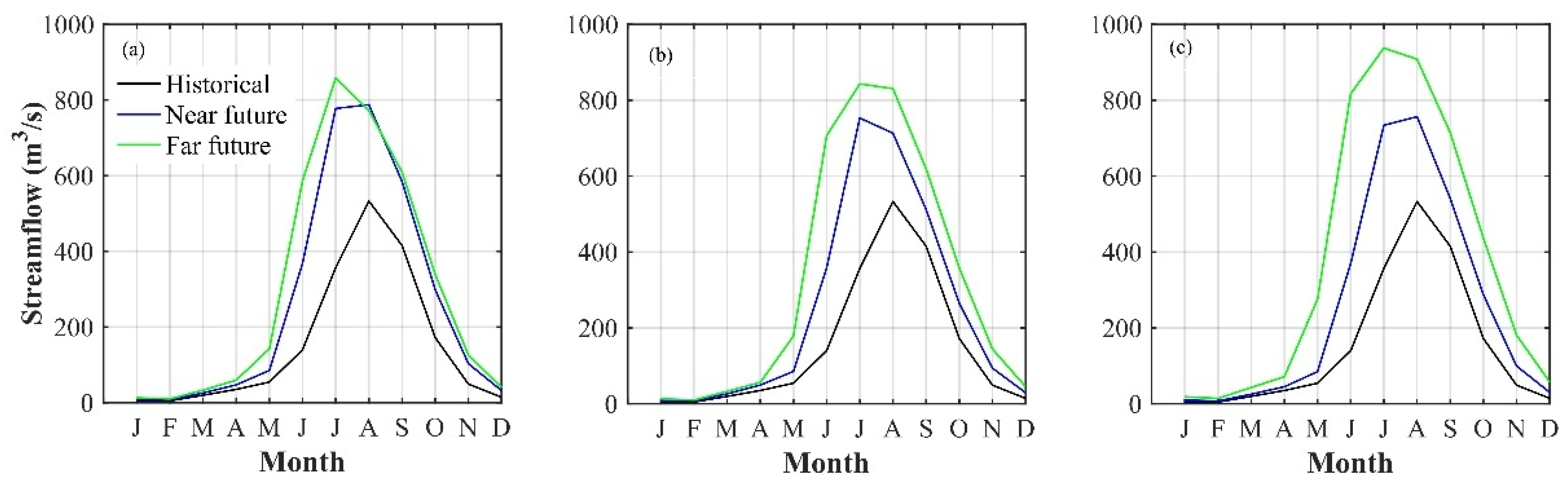
3.4.1. Annual and Monthly Streamflow to Changing Climate
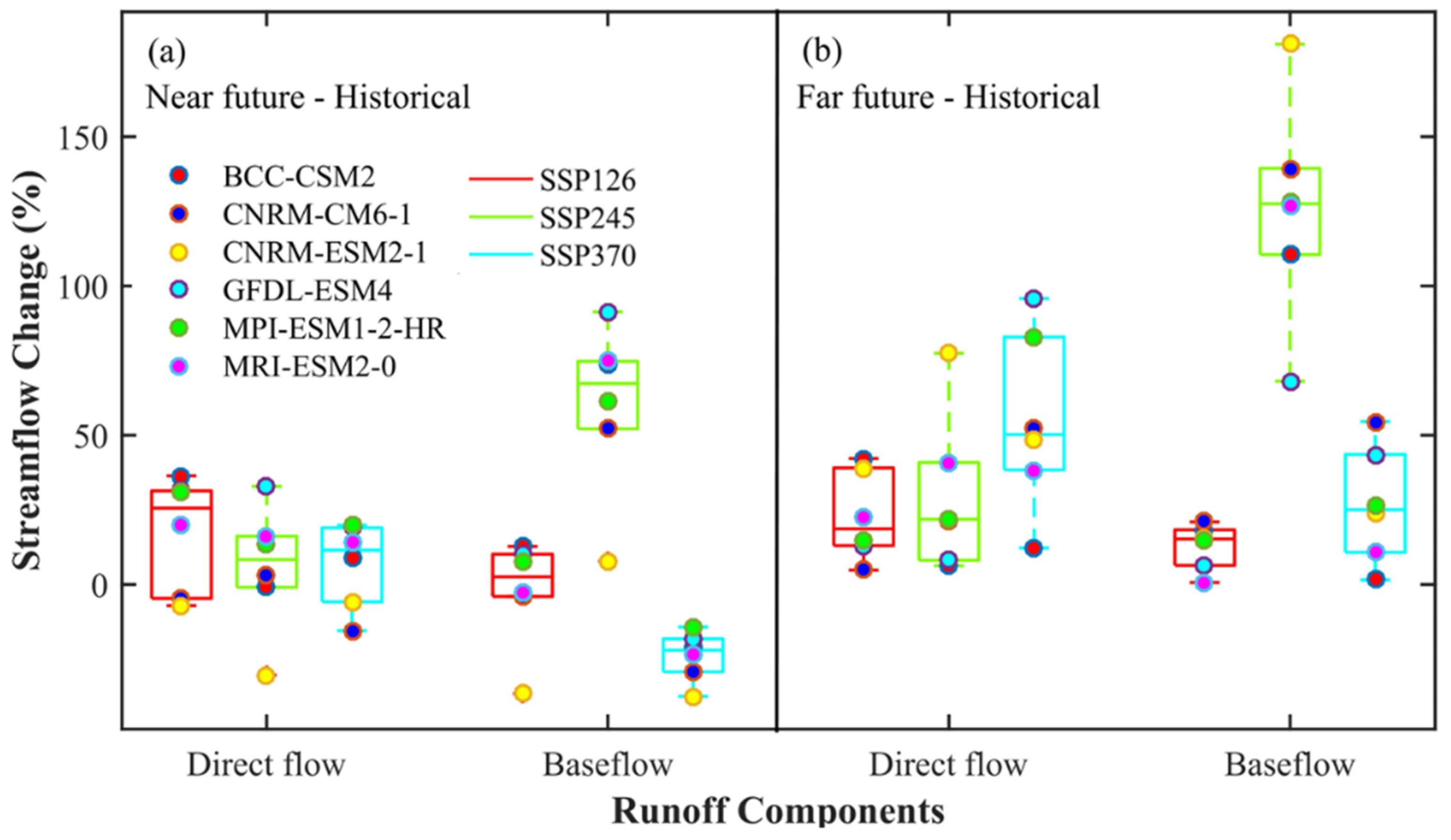
3.4.2. Changes in Streamflow Components to Changing Climate
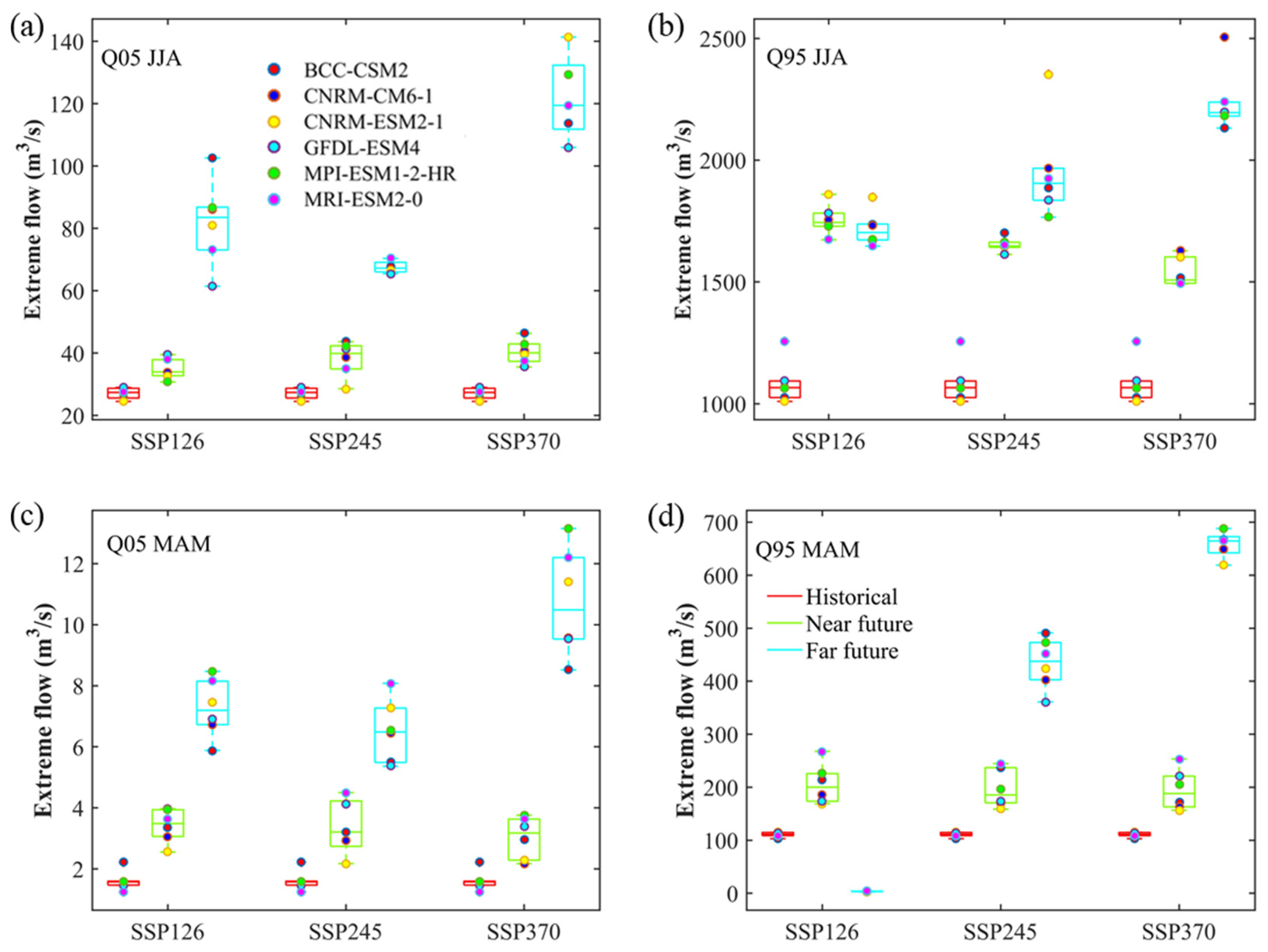
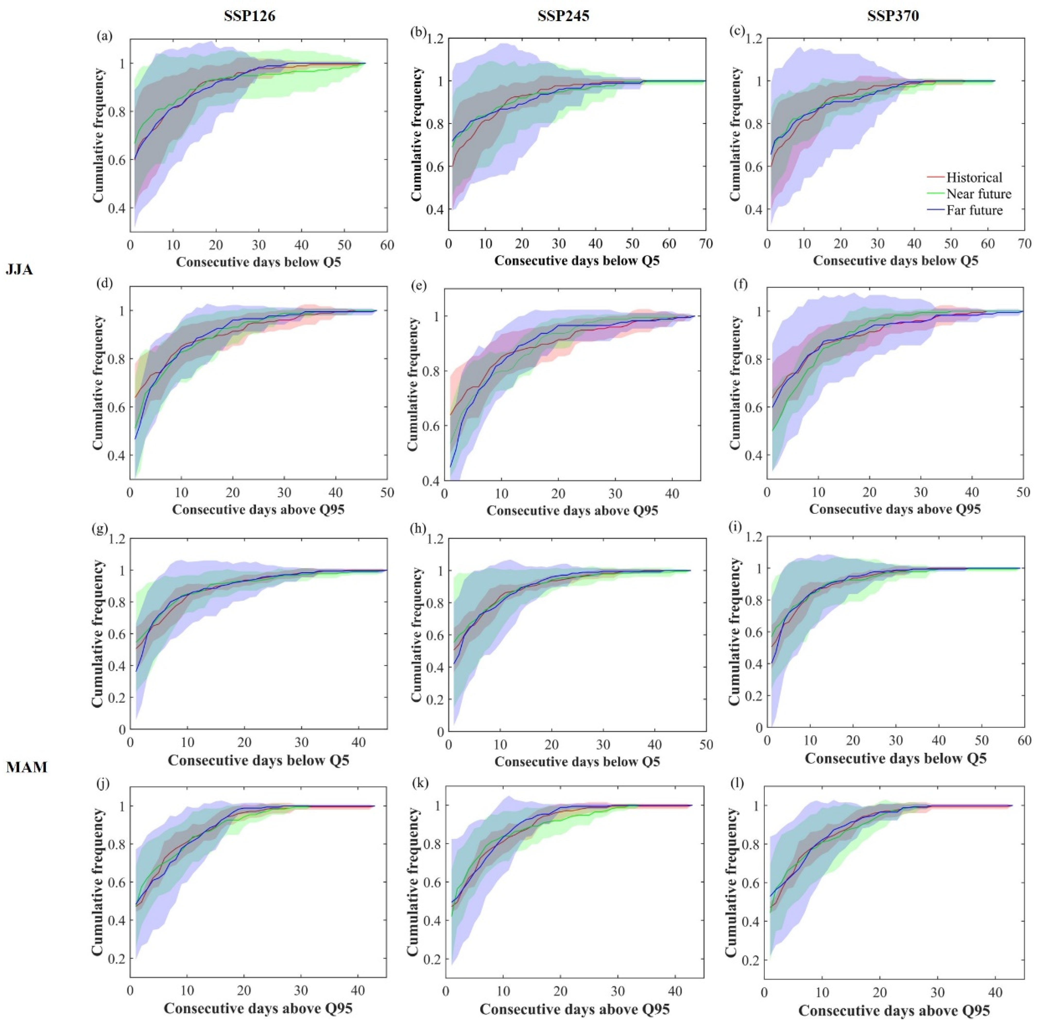
3.4.3. Extreme Flows
4. Discussion
4.1. Application of Hydrological Model
4.2. The Applicability of CMIP6 Models and Bias Correction Methods in the Arid Area of Northwest China
4.3. Climate Change Impacts on Runoff
5. Conclusions
Supplementary Materials
Author Contributions
Funding
Institutional Review Board Statement
Informed Consent Statement
Data Availability Statement
Acknowledgments
Conflicts of Interest
References
- Müller Schmied, H.; Adam, L.; Eisner, S.; Fink, G.; Flörke, M.; Kim, H.; Oki, T.; Portmann, F.T.; Reinecke, R.; Riedel, C.; et al. Variations of global and continental water balance components as impacted by climate forcing uncertainty and human water use. Hydrol. Earth Syst. Sci. 2016, 20, 2877–2898. [Google Scholar] [CrossRef] [Green Version]
- Han, H.; Wang, R. Landscape pattern change research of Yarkant irrigated area. In Proceedings of the 2012 International Symposium on Geomatics for Integrated Water Resource Management, Lanzhou, China, 19–21 October 2012; pp. 1–4. [Google Scholar]
- Huang, S.; Wortmann, M.; Duethmann, D.; Menz, C.; Shi, F.; Zhao, C.; Su, B.; Krysanova, V. Adaptation strategies of agriculture and water management to climate change in the Upper Tarim River basin, NW China. Agric. Water Manag. 2018, 203, 207–224. [Google Scholar] [CrossRef]
- Xiang, Y.; Wang, Y.; Chen, Y.; Bai, Y.; Zhang, L.; Zhang, Q. Hydrological Drought Risk Assessment Using a Multidimensional Copula Function Approach in Arid Inland Basins, China. Water 2020, 12, 1888. [Google Scholar] [CrossRef]
- Xu, J.; Chen, Y.; Li, W.; Nie, Q.; Song, C.; Wei, C. Integrating Wavelet Analysis and BPANN to Simulate the Annual Runoff With Regional Climate Change: A Case Study of Yarkand River, Northwest China. Water Resour. Manag. 2014, 28, 2523–2537. [Google Scholar] [CrossRef]
- Held, I.M.; Soden, B.J. Robust Responses of the Hydrological Cycle to Global Warming. J. Clim. 2006, 19, 5686–5699. [Google Scholar] [CrossRef]
- Barnett, T.P.; Adam, J.C.; Lettenmaier, D.P. Potential impacts of a warming climate on water availability in snow-dominated regions. Nature 2005, 438, 303–309. [Google Scholar] [CrossRef]
- Lutz, A.F.; Immerzeel, W.W.; Shrestha, A.B.; Bierkens, M.F.P. Consistent increase in High Asia’s runoff due to increasing glac-ier melt and precipitation. Nat. Clim. Chang. 2014, 4, 587–592. [Google Scholar] [CrossRef] [Green Version]
- Ragettli, S.; Immerzeel, W.W.; Pellicciotti, F. Contrasting climate change impact on river flows from high-altitude catch-ments in the Himalayan and Andes Mountains. Proc. Natl. Acad. Sci. USA 2016, 113, 6. [Google Scholar] [CrossRef] [PubMed] [Green Version]
- Sun, C.; Yang, J.; Chen, Y.; Li, X.; Yang, Y.; Zhang, Y. Comparative study of streamflow components in two inland rivers in the Tianshan Mountains, Northwest China. Environ. Earth Sci. 2016, 75, 9. [Google Scholar] [CrossRef]
- Bi, Y.; Hongjie, X.; Chunlin, H.; Changqing, K. Snow Cover Variations and Controlling Factors at Upper Heihe River Basin, Northwestern China. Remote Sens. 2015, 7, 6741–6762. [Google Scholar] [CrossRef] [Green Version]
- Wang, W.; Huang, X.; Deng, J.; Xie, H.; Liang, T. Spatio-Temporal Change of Snow Cover and Its Response to Climate over the Tibetan Plateau Based on an Improved Daily Cloud-Free Snow Cover Product. Remote Sens. 2015, 7, 169–194. [Google Scholar] [CrossRef]
- Tobias, S.; Thomas, B.; Renaud, G.; Scott, S.; Andrew, W.R.; Justin, M.; Peter, B.-G.; Andrey, Y. Will climate change exacerbate water stress in? Clim. Chang. 2012, 122, 881–899. [Google Scholar]
- Chen, F.; Chen, Y.; Bakhtiyorov, Z.; Zhang, H.; Man, W.; Chen, F. Central Asian river streamflows have not continued to increase during the recent warming hiatus. Atmos. Res. 2020, 246, 105–124. [Google Scholar] [CrossRef]
- Tosunoğlu, F.; Onof, C. Joint modelling of drought characteristics derived from historical and synthetic rainfalls: Application of Generalized Linear Models and Copulas. J. Hydrol.—Reg. Stud. 2017, 14, 167–181. [Google Scholar] [CrossRef]
- Zhang, S.; Gao, X.; Zhang, X.; Hagemann, S. Projection of glacier runoff in Yarkant River basin and Beida River basin, Western China. Hydrol. Processes 2012, 26, 2773–2781. [Google Scholar] [CrossRef]
- Luo, Y.; Wang, X.; Piao, S.; Sun, L.; Ciais, P.; Zhang, Y.; Ma, C.; Gan, R.; He, C. Contrasting streamflow regimes induced by melting glaciers across the Tien Shan—Pamir—North Karakoram. Sci. Rep. 2018, 8, 16470. [Google Scholar] [CrossRef] [PubMed]
- Azmat, M.; Qamar, M.U.; Huggel, C.; Hussain, E. Future climate and cryosphere impacts on the hydrology of a scarcely gauged catchment on the Jhelum river basin, Northern Pakistan. Sci. Total Environ. 2018, 639, 961–976. [Google Scholar] [CrossRef]
- Li, S.-Y.; Miao, L.-J.; Jiang, Z.-H.; Wang, G.-J.; Gnyawali, K.R.; Zhang, J.; Zhang, H.; Fang, K.; He, Y.; Li, C. Projected drought conditions in Northwest China with CMIP6 models under combined SSPs and RCPs for 2015–2099. Adv. Clim. Chang. Res. 2020, 11, 210–217. [Google Scholar] [CrossRef]
- Chen, Y.; Li, W.; Fang, G.; Li, Z. Review article: Hydrological modeling in glacierized catchments of central Asia—status and challenges. Hydrol. Earth Syst. Sci. 2017, 21, 669–684. [Google Scholar] [CrossRef] [Green Version]
- U.S. Army Corps of Enginers Hydrologic Engineering Center. Hydrologic Modeling System HEC-HMS User’s Manual; US Army Corps of Engineers, Hydrologic Engineering Center: Davis, CA, USA, 2016. [Google Scholar]
- Azmat, M.; Choi, M.; Kim, T.-W.; Liaqat, U.W. Hydrological modeling to simulate streamflow under changing climate in a scarcely gauged cryosphere catchment. Environ. Earth Sci. 2016, 75, 186. [Google Scholar] [CrossRef]
- Fazel, K.; Scharffenberg, W.A.; Bombardelli, F.A. Assessment of the Melt Rate Function in a Temperature Index Snow Model Using Observed Data. J. Hydrol. Eng. 2014, 19, 1275–1282. [Google Scholar] [CrossRef]
- Konapala, G.; Mishra, A.K.; Wada, Y.; Mann, M.E. Climate change will affect global water availability through compounding changes in seasonal precipitation and evaporation. Nat. Commun. 2020, 11, 3044. [Google Scholar] [CrossRef] [PubMed]
- Laurent, L.; Buoncristiani, J.-F.; Pohl, B.; Zekollari, H.; Farinotti, D.; Huss, M.; Mugnier, J.-L.; Pergaud, J. The impact of climate change and glacier mass loss on the hydrology in the Mont-Blanc massif. Sci. Rep. 2020, 10, 10420. [Google Scholar] [CrossRef]
- Xu, Y.; Zhang, X.; Wang, X.; Hao, Z.; Singh, V.P.; Hao, F. Propagation from meteorological drought to hydrological drought under the impact of human activities: A case study in northern China. J. Hydrol. 2019, 579, 124147. [Google Scholar] [CrossRef]
- Chen, Y.; Liu, A.; Zhang, Z.; Hope, C.; Crabbe, M.J.C. Economic losses of carbon emissions from circum-Arctic permafrost regions under RCP-SSP scenarios. Sci. Total Environ. 2019, 658, 1064–1068. [Google Scholar] [CrossRef]
- Moss, R.H.; Edmonds, J.A.; Hibbard, K.A.; Manning, M.R.; Rose, S.K.; van Vuuren, D.P.; Carter, T.R.; Emori, S.; Kainuma, M.; Kram, T. The next generation of scenarios for climate change research and assessment. Nature 2010, 463, 747–756. [Google Scholar] [CrossRef] [PubMed]
- Almazroui, M.; Saeed, F.; Saeed, S.; Nazrul Islam, M.; Ismail, M.; Klutse, N.A.B.; Siddiqui, M.H. Projected Change in Temperature and Precipitation Over Africa from CMIP6. Earth Syst. Environ. 2020, 4, 455–475. [Google Scholar] [CrossRef]
- Parsons, L.A. Implications of CMIP6 Projected Drying Trends for 21st Century Amazonian Drought Risk. Earth’s Future 2020, 8, e2020EF001608. [Google Scholar] [CrossRef]
- Church, J.A.; Clark, P.U.; Cazenave, A.; Gregory, J.M.; Jevrejeva, S.; Levermann, A.; Merrifield, M.A.; Milne, G.A.; Nerem, R.S.; Nunn, P.D.; et al. Sea Level Change. In Climate Change 2013: The Physical Science Basis. Contribution of Working Group I to the Fifth Assessment Report of the Intergovernmental Panel on Climate Change; Stocker, T.F., Qin, D., Plattner, G.-K., Tignor, M., Allen, S.K., Boschung, J., Nauels, A., Xia, Y., Bex, V., Midgley, P.M., Eds.; Cambridge University Press: Cambridge, UK; New York, NY, USA, 2013; Volume 26, pp. 1137–1216. [Google Scholar]
- O’Neill, B.C.; Kriegler, E.; Riahi, K.; Ebi, K.L.; Hallegatte, S.; Carter, T.R.; Mathur, R.; van Vuuren, D.P. A new scenario framework for climate change research: The concept of shared socioeconomic pathways. Clim. Change 2013, 122, 387–400. [Google Scholar] [CrossRef] [Green Version]
- Kan, B.; Su, F.; Xu, B.; Xie, Y.; Li, J.; Zhang, H. Generation of High Mountain Precipitation and Temperature Data for a Quantitative Assessment of Flow Regime in the Upper Yarkant Basin in the Karakoram. J. Geophys. Res. Atmos. 2018, 123, 8462–8486. [Google Scholar] [CrossRef]
- Chen, Y.; Xu, C.; Chen, Y.; Li, W.; Liu, J. Response of glacial-lake outburst floods to climate change in the Yarkant River basin on northern slope of Karakoram Mountains, China. Quat. Int. 2010, 226, 75–81. [Google Scholar] [CrossRef]
- Li, B.; Chen, Y.; Chipman, J.W.; Shi, X.; Chen, Z. Why does the runoff in Hotan River show a slight decreased trend in northwestern China? Atmos. Sci. Lett. 2018, 19, e800. [Google Scholar] [CrossRef] [Green Version]
- Che, T.; Xin, L.; Jin, R.; Armstrong, R.; Zhang, T. Snow depth derived from passive microwave remote-sensing data in China. Ann. Glaciol. 2008, 49, 145–154. [Google Scholar] [CrossRef] [Green Version]
- Dai, L. Inter-Calibrating SMMR, SSM/I and SSMI/S Data to Improve the Consistency of Snow-Depth Products in China. Remote Sens. 2015, 7, 7212–7230. [Google Scholar] [CrossRef] [Green Version]
- Liyun, D.; Tao, C.; Yongjian, D.; Xiaohua, H. Evaluation of snow cover and snow depth on the Qinghai–Tibetan Plateau derived from passive microwave remote sensing. Cryosphere 2017, 11, 1933–1948. [Google Scholar]
- Redding, D.W.; Atkinson, P.M.; Cunningham, A.A.; Lo Iacono, G.; Moses, L.M.; Wood, J.L.N.; Jones, K.E. Impacts of environmental and socio-economic factors on emergence and epidemic potential of Ebola in Africa. Nat. Commun. 2019, 10, 4531. [Google Scholar] [CrossRef]
- O’Neill, B.C.; Kriegler, E.; Ebi, K.L.; Kemp-Benedict, E.; Riahi, K.; Rothman, D.S.; van Ruijven, B.J.; van Vuuren, D.P.; Birkmann, J.; Kok, K.; et al. The roads ahead: Narratives for shared socioeconomic pathways describing world futures in the 21st century. Glob. Environ. Chang. 2017, 42, 169–180. [Google Scholar] [CrossRef] [Green Version]
- Chen, Y.; Li, X.; Huang, K.; Luo, M.; Gao, M. High-Resolution Gridded Population Projections for China Under the Shared Socioeconomic Pathways. Earth’s Future 2020, 8, e2020EF001491. [Google Scholar] [CrossRef]
- O’Neill, B.C.; Tebaldi, C.; van Vuuren, D.P.; Eyring, V.; Friedlingstein, P.; Hurtt, G.; Knutti, R.; Kriegler, E.; Lamarque, J.-F.; Lowe, J.; et al. The Scenario Model Intercomparison Project (ScenarioMIP) for CMIP6. Geosci. Model Dev. 2016, 9, 3461–3482. [Google Scholar] [CrossRef] [Green Version]
- Halwatura, D.; Najim, M.M.M. Application of the HEC-HMS model for runoff simulation in a tropical catchment. Environ. Modell. Softw. 2013, 46, 155–162. [Google Scholar] [CrossRef]
- Tassew, B.G.; Belete, M.A.; Miegel, K. Application of HEC-HMS Model for Flow Simulation in the Lake Tana Basin: The Case of Gilgel Abay Catchment, Upper Blue Nile Basin, Ethiopia. Hydrology 2019, 6, 21. [Google Scholar] [CrossRef] [Green Version]
- Meenu, R.; Rehana, S.; Mujumdar, P.P. Assessment of hydrologic impacts of climate change in Tunga-Bhadra river basin, India with HEC-HMS and SDSM. Hydrol. Process. 2013, 27, 1572–1589. [Google Scholar] [CrossRef]
- Zhao, Q.; Zhang, S.; Ding, Y.J.; Wang, J.; Han, H.; Xu, J.; Zhao, C.; Guo, W.; Shangguan, D. Modeling Hydrologic Response to Climate Change and Shrinking Glaciers in the Highly Glacierized Kunma Like River Catchment, Central Tian Shan. J. Hydrometeorol. 2015, 16, 2383–2402. [Google Scholar] [CrossRef]
- Moriasi, D.N.; Arnold, J.G.; Van Liew, M.W.; Bingner, R.L.; Harmel, R.D.; Veith, T.L. Model evaluation guidelines for systematic quantification of accuracy in watershed simulations. Trans. ASABE 2007, 50, 885–900. [Google Scholar] [CrossRef]
- Li, L.; Shen, M.; Hou, Y.; Xu, C.-Y.; Lutz, A.F.; Chen, J.; Jain, S.K.; Li, J.; Chen, H. Twenty-first-century glacio-hydrological changes in the Himalayan headwater Beas River basin. Hydrol. Earth Syst. Sci. 2019, 23, 1483–1503. [Google Scholar] [CrossRef] [Green Version]
- Sorg, A.; Bolch, T.; Stoffel, M.; Solomina, O.; Beniston, M. Climate change impacts on glaciers and runoff in Tien Shan (Central Asia). Nat. Clim. Change 2012, 2, 725–731. [Google Scholar] [CrossRef]
- Hall, F.R. Base flow recessions—A review. Water Resour. Res. 1968, 4, 973–983. [Google Scholar] [CrossRef]
- Fan, Y.; Chen, Y.; Liu, Y.; Li, W. Variation of baseflows in the headstreams of the Tarim River Basin during 1960–2007. J. Hydrol. 2013, 487, 98–108. [Google Scholar] [CrossRef]
- Viola, M.R.; de Mello, C.R.; Chou, S.C.; Yanagi, S.N.; Gomes, J.L. Assessing climate change impacts on Upper Grande River Basin hydrology, Southeast Brazil. Int. J. Climatol. 2015, 35, 1054–1068. [Google Scholar] [CrossRef]
- Kong, X.; Li, Z.; Liu, Z. Flood Prediction in Ungauged Basins by Physical-Based TOPKAPI Model. Adv. Meteorol. 2019, 2019, 4795853. [Google Scholar] [CrossRef]
- Wi, S.; Yang, Y.C.E.; Steinschneider, S.; Khalil, A.; Brown, C.M. Calibration approaches for distributed hydrologic models in poorly gaged basins: Implication for streamflow projections under climate change. Hydrol. Earth Syst. Sci. 2015, 19, 857–876. [Google Scholar] [CrossRef] [Green Version]
- Fang, G.; Yang, J.; Chen, Y.; Li, Z.; Ji, H.; De Maeyer, P. How Hydrologic Processes Differ Spatially in a Large Basin: Multisite and Multiobjective Modeling in the Tarim River Basin. J. Geophys. Res. Atmos. 2018, 123, 7079–7113. [Google Scholar] [CrossRef]
- Zhang, F.; Bai, L.; Li, L.; Wang, Q. Sensitivity of runoff to climatic variability in the northern and southern slopes of the Middle Tianshan Mountains, China. J. Arid Land 2016, 8, 681–693. [Google Scholar] [CrossRef] [Green Version]
- Parsons, L.A.; Brennan, M.K.; Wills, R.C.J.; Proistosescu, C. Magnitudes and Spatial Patterns of Interdecadal Temperature Variability in CMIP6. Geophys. Res. Lett. 2020, 47, e2019GL086588. [Google Scholar] [CrossRef]
- Xin, X.; Wu, T.; Zhang, J.; Yao, J.; Fang, Y. Comparison of CMIP6 and CMIP5 simulations of precipitation in China and the East Asian summer monsoon. Int. J. Climatol. 2020, 40, 6423–6440. [Google Scholar] [CrossRef] [Green Version]
- Bai, H.; Xiao, D.; Wang, B.; Liu, D.L.; Feng, P.; Tang, J. Multi-model ensemble of CMIP6 projections for future extreme climate stress on wheat in the North China plain. Int. J. Climatol. 2020, 41, E171–E186. [Google Scholar] [CrossRef]
- Mishra, V.; Bhatia, U.; Tiwari, A.D. Bias-corrected climate projections for South Asia from Coupled Model Intercomparison Project-6. Sci. Data 2020, 7, 338. [Google Scholar] [CrossRef]
- Yao, N.; Li, Y.; Li, N.; Yang, D.; Ayantobo, O.O. Bias correction of precipitation data and its effects on aridity and drought assessment in China over 1961–2015. Sci. Total Environ. 2018, 639, 1015–1027. [Google Scholar] [CrossRef] [PubMed]
- Meyer, J.; Kohn, I.; Stahl, K.; Hakala, K.; Seibert, J.; Cannon, A.J. Effects of univariate and multivariate bias correction on hydrological impact projections in alpine catchments. Hydrol. Earth Syst. Sci. 2019, 23, 1339–1354. [Google Scholar] [CrossRef] [Green Version]
- Chen, Y.; Li, Z.; Fan, Y.; Wang, H.; Deng, H. Progress and prospects of climate change impacts on hydrology in the arid region of northwest China. Environ. Res. 2015, 139, 11–19. [Google Scholar] [CrossRef]
- Ji, F.; Wu, Z.; Huang, J.; Chassignet, E.P. Evolution of land surface air temperature trend. Nat. Clim. Chang. 2014, 4, 462–466. [Google Scholar] [CrossRef]
- Tian, D.; Guo, Y.; Dong, W. Future changes and uncertainties in temperature and precipitation over China based on CMIP5 models. Adv. Atmos. Sci. 2015, 32, 487–496. [Google Scholar] [CrossRef]
- Wang, L.; Chen, W. A CMIP5 multimodel projection of future temperature, precipitation, and climatological drought in China. Int. J. Climatol. 2014, 34, 2059–2078. [Google Scholar] [CrossRef]
- Li, Z.; Fang, G.; Chen, Y.; Duan, W.; Mukanov, Y. Agricultural water demands in Central Asia under 1.5 °C and 2.0 °C global warming. Agric. Water Manag. 2020, 231, 106020. [Google Scholar] [CrossRef]
- Li, Z.; Feng, Q.; Li, Z.; Yuan, R.; Gui, J.; Lv, Y. Climate background, fact and hydrological effect of multiphase water transformation in cold regions of the Western China: A review. Earth-Sci. Rev. 2019, 190, 33–57. [Google Scholar]
- Shen, Y.-J.; Shen, Y.; Fink, M.; Kralisch, S.; Chen, Y.; Brenning, A. Trends and variability in streamflow and snowmelt runoff timing in the southern Tianshan Mountains. J. Hydrol. 2018, 557, 173–181. [Google Scholar] [CrossRef]
- Wang, Y.-J.; Qin, D.-H. Influence of climate change and human activity on water resources in arid region of Northwest China: An overview. Adv. Clim. Chang. Res. 2017, 8, 268–278. [Google Scholar] [CrossRef]
- Adnan, M.; Nabi, G.; Saleem Poomee, M.; Ashraf, A. Snowmelt runoff prediction under changing climate in the Himalayan cryosphere: A case of Gilgit River Basin. Geosci. Front. 2017, 8, 941–949. [Google Scholar] [CrossRef] [Green Version]
- Liu, J.; Shen, B.; Li, H. Dynamics of major hydro-climatic variables in the headwater catchment of the Tarim River Basin, Xinjiang, China. Quat. Int. 2015, 380–381, 143–148. [Google Scholar] [CrossRef]
- Wang, C.; Xu, J.; Chen, Y.; Bai, L.; Chen, Z. A hybrid model to assess the impact of climate variability on streamflow for an ungauged mountainous basin. Clim. Dynam. 2017, 50, 2829–2844. [Google Scholar] [CrossRef]
- Bajracharya, A.R.; Bajracharya, S.R.; Shrestha, A.B.; Maharjan, S.B. Climate change impact assessment on the hydrological regime of the Kaligandaki Basin, Nepal. Sci. Total Environ. 2018, 625, 837–848. [Google Scholar] [CrossRef] [PubMed]
- Schmidli, J.; Frei, C.; Vidale, P.L. Downscaling from GCM precipitation: A benchmark for dynamical and statistical downscaling methods. Int. J. Climatol. 2006, 26, 679–689. [Google Scholar] [CrossRef]
- Bayazit, Y.; Bakiş, R.; Koç, C. Mapping Distribution of Precipitation, Temperature and Evaporation in Seydisuyu Basin with the Help of Distance Related Estimation Methods. J. Geogr. Inform. Syst. 2016, 08, 224–237. [Google Scholar] [CrossRef] [Green Version]
- Leander, R.; Buishand, T.A. Resampling of regional climate model output for the simulation of extreme river flows. J. Hydrol. 2007, 332, 487–496. [Google Scholar] [CrossRef]


| ID | Model Name | Country | Institution | Resolution |
|---|---|---|---|---|
| 1 | BCC-CSM2 | China | Beijing Climate Center | 100 km |
| 2 | CNRM-CM6-1 | France | Centre National de Recherches Météorologiques | 100 km |
| 3 | CNRM-ESM2-1 | France | Centre National de Recherches Météorologiques | 250 km |
| 4 | GFDL-ESM4 | America | Geophysical Fluid Dynamics Laboratory | 250 km |
| 5 | MPI-ESM1-2-HR | Germany | Max Planck Institute for Meteorology | 100 km |
| 6 | MRI-ESM2-0 | Japan | Meteorological Research Institute | 100 km |
| Bias Correction for Temperature | Bias Correction for Precipitation |
|---|---|
| Linear scaling (LS) | Power transformation (PT) |
| Distribution mapping for temperature using Gaussian distribution (DM) | Local intensity scaling (LOCI) |
| Distribution mapping for precipitation using gamma distribution (DM) |
| Time Periods | NSE | PBIAS (%) | R2 |
|---|---|---|---|
| Calibration period (2005–2010) | 0.80 | 5.86 | 0.81 |
| Validation period (1986–2004) | 0.72 | 16.56 | 0.70 |
| Validation period (2011–2014) | 0.83 | 9.74 | 0.85 |
| CMIP6 Models | Frequency-Based Statistics | Time-Series-Based Metrics | |||||||
|---|---|---|---|---|---|---|---|---|---|
| Mean (°C) | Median (°C) | Standard Deviation (°C) | 10th Percentile (°C) | 99th Percentile (°C) | R2 | RMSE | MAE | ||
| BCC | Obs | 3.98 | 5.60 | 10.60 | −10.77 | 16.70 | |||
| Raw | 4.84 | 4.21 | 10.43 | −18.96 | 18.60 | 0.84 | 10.62 | 9.28 | |
| LS | 3.98 | 5.85 | 10.72 | −11.37 | 16.73 | 0.87 | 5.54 | 4.22 | |
| DM | 3.98 | 5.77 | 10.60 | −11.13 | 16.47 | 0.87 | 5.38 | 4.01 | |
| NERM-CM6-1 | Obs | 3.98 | 5.60 | 10.60 | −10.77 | 16.70 | |||
| Raw | 2.93 | 1.45 | 6.85 | −12.25 | 14.55 | 0.51 | 11.58 | 9.86 | |
| LS | 3.98 | 6.06 | 10.99 | −11.25 | 16.41 | 0.82 | 6.51 | 4.79 | |
| DM | 3.98 | 5.43 | 10.60 | −10.53 | 16.62 | 0.85 | 5.80 | 4.34 | |
| CNRM-ESM2-1 | Obs | 3.98 | 5.60 | 10.60 | −10.77 | 16.70 | |||
| Raw | 1.15 | 0.35 | 6.44 | −9.55 | 16.55 | 0.51 | 10.49 | 8.78 | |
| LS | 3.98 | 5.66 | 10.69 | −10.80 | 16.51 | 0.85 | 5.83 | 4.31 | |
| DM | 3.98 | 5.45 | 10.60 | −10.34 | 16.62 | 0.86 | 5.62 | 4.20 | |
| GFDL-ESM4 | Obs | 3.98 | 5.60 | 10.60 | −10.77 | 16.70 | |||
| Raw | 7.12 | 3.85 | 11.06 | −20.95 | 11.45 | 0.47 | 15.76 | 12.53 | |
| LS | 3.98 | 6.53 | 13.35 | −12.96 | 16.12 | 0.68 | 9.86 | 5.51 | |
| DM | 3.98 | 5.57 | 10.60 | −10.07 | 16.11 | 0.86 | 5.62 | 4.16 | |
| MPI-ESM1-2-HR | Obs | 3.98 | 5.60 | 10.60 | −10.77 | 16.70 | |||
| Raw | 4.00 | 2.25 | 6.92 | −13.15 | 13.05 | 0.53 | 12.10 | 10.39 | |
| LS | 3.98 | 6.29 | 11.05 | −11.35 | 16.32 | 0.82 | 6.45 | 4.64 | |
| DM | 3.98 | 5.47 | 10.60 | −10.35 | 16.70 | 0.86 | 5.62 | 4.19 | |
| MRI-ESM2-0 | Obs | 3.98 | 5.60 | 10.60 | −10.77 | 16.70 | |||
| Raw | 3.41 | 0.85 | 8.25 | −15.55 | 14.25 | 0.52 | 12.01 | 10.15 | |
| LS | 3.98 | 6.69 | 11.56 | −11.56 | 16.08 | 0.81 | 6.89 | 4.99 | |
| DM | 3.98 | 5.57 | 10.60 | −9.89 | 16.32 | 0.87 | 5.33 | 4.04 | |
| CMIP6 Models | Frequency-Based Statistics | Time-Series-Based Metrics | |||||||
|---|---|---|---|---|---|---|---|---|---|
| Mean (mm) | Median (mm) | Standard Deviation (mm) | 10th Percentile (mm) | Fre-Quency of Wet Days (%) | Intensity of Wet Days (mm) | RMSE | MAE | ||
| BCC | Obs | 0.23 | 0.00 | 1.12 | 0.20 | 0.05 | 1.17 | ||
| Raw | 1.52 | 0.53 | 2.50 | 4.24 | 0.39 | 3.54 | 3.00 | 1.59 | |
| PT | 0.23 | 0.00 | 1.09 | 0.39 | 0.05 | 3.25 | 1.53 | 0.41 | |
| LOCI | 0.23 | 0.00 | 0.76 | 1.04 | 0.10 | 2.08 | 1.32 | 0.41 | |
| DM | 0.11 | 0.00 | 0.57 | 0.22 | 0.03 | 2.47 | 1.24 | 0.31 | |
| CNRM-CM6-1 | Obs | 0.23 | 0.00 | 1.12 | 0.20 | 0.05 | 1.17 | ||
| Raw | 1.52 | 0.53 | 2.19 | 4.24 | 0.40 | 3.14 | 2.80 | 1.60 | |
| PT | 0.23 | 0.01 | 1.13 | 0.30 | 0.05 | 3.73 | 1.59 | 0.42 | |
| LOCI | 0.20 | 0.00 | 0.67 | 0.92 | 0.09 | 1.94 | 1.31 | 0.40 | |
| DM | 0.21 | 0.00 | 1.29 | 0.17 | 0.04 | 4.11 | 1.71 | 0.42 | |
| CNRM-ESM2-1 | Obs | 0.23 | 0.00 | 1.12 | 0.20 | 0.05 | 1.17 | ||
| Raw | 1.60 | 0.80 | 2.38 | 3.90 | 0.42 | 3.28 | 2.98 | 1.69 | |
| PT | 0.23 | 0.01 | 1.15 | 0.29 | 0.05 | 3.73 | 1.59 | 0.42 | |
| LOCI | 0.19 | 0.00 | 0.70 | 0.87 | 0.09 | 2.08 | 1.32 | 0.40 | |
| DM | 0.23 | 0.00 | 1.54 | 0.13 | 0.04 | 4.80 | 1.90 | 0.44 | |
| GFDL-ESM4 | Obs | 0.23 | 0.00 | 1.12 | 0.20 | 0.05 | 1.17 | ||
| Raw | 1.35 | 0.70 | 1.94 | 3.30 | 0.35 | 3.04 | 2.51 | 1.44 | |
| PT | 0.23 | 0.01 | 1.19 | 0.30 | 0.05 | 4.61 | 1.60 | 0.41 | |
| LOCI | 0.23 | 0.00 | 0.68 | 0.96 | 0.10 | 1.92 | 1.30 | 0.40 | |
| DM | 0.20 | 0.00 | 1.35 | 0.14 | 0.04 | 4.13 | 1.74 | 0.41 | |
| MPI-ESM1-2-HR | Obs | 0.23 | 0.00 | 1.12 | 0.20 | 0.05 | 1.17 | ||
| Raw | 1.51 | 0.70 | 2.19 | 3.70 | 0.40 | 3.14 | 2.80 | 1.60 | |
| PT | 0.23 | 0.01 | 1.13 | 0.30 | 0.05 | 3.65 | 1.58 | 0.42 | |
| LOCI | 0.23 | 0.00 | 0.67 | 0.92 | 0.09 | 1.94 | 1.31 | 0.40 | |
| DM | 0.21 | 0.00 | 1.29 | 0.17 | 0.04 | 4.11 | 1.71 | 0.42 | |
| MRI-ESM2-0 | Obs | 0.23 | 0.00 | 1.12 | 0.20 | 0.05 | 1.17 | ||
| Raw | 1.59 | 0.80 | 2.19 | 3.80 | 0.42 | 3.12 | 2.82 | 1.67 | |
| PT | 0.23 | 0.01 | 1.17 | 0.30 | 0.05 | 3.65 | 1.58 | 0.42 | |
| LOCI | 0.17 | 0.00 | 0.67 | 0.90 | 0.09 | 1.95 | 1.29 | 0.40 | |
| DM | 0.23 | 0.00 | 1.65 | 0.12 | 0.04 | 4.99 | 1.96 | 0.44 | |
| Variables | SSPs | Near Term (2021–2049) | Far Term (2071–2099) |
|---|---|---|---|
| Temperature (°C) | SSP126 | 1.72 | 3.76 |
| SSP245 | 1.79 | 4.29 | |
| SSP370 | 1.75 | 6.22 | |
| Precipitation (mm (%)) | SSP126 | 9.90 (11.95) | 11.52 (14.82) |
| SSP245 | 9.94 (12.00) | 13.33 (16.09) | |
| SSP370 | 8.95 (10.79) | 24.09 (29.07) | |
| Streamflow (%) | SSP126 | 19.20 | 36.69 |
| SSP245 | 10.62 | 46.11 | |
| SSP370 | 14.01 | 70.40 |
Publisher’s Note: MDPI stays neutral with regard to jurisdictional claims in published maps and institutional affiliations. |
© 2021 by the authors. Licensee MDPI, Basel, Switzerland. This article is an open access article distributed under the terms and conditions of the Creative Commons Attribution (CC BY) license (https://creativecommons.org/licenses/by/4.0/).
Share and Cite
Xiang, Y.; Wang, Y.; Chen, Y.; Zhang, Q. Impact of Climate Change on the Hydrological Regime of the Yarkant River Basin, China: An Assessment Using Three SSP Scenarios of CMIP6 GCMs. Remote Sens. 2022, 14, 115. https://doi.org/10.3390/rs14010115
Xiang Y, Wang Y, Chen Y, Zhang Q. Impact of Climate Change on the Hydrological Regime of the Yarkant River Basin, China: An Assessment Using Three SSP Scenarios of CMIP6 GCMs. Remote Sensing. 2022; 14(1):115. https://doi.org/10.3390/rs14010115
Chicago/Turabian StyleXiang, Yanyun, Yi Wang, Yaning Chen, and Qifei Zhang. 2022. "Impact of Climate Change on the Hydrological Regime of the Yarkant River Basin, China: An Assessment Using Three SSP Scenarios of CMIP6 GCMs" Remote Sensing 14, no. 1: 115. https://doi.org/10.3390/rs14010115