
Analysis of Operational Effects of Bus Lanes with Intermittent Priority with Spatio-Temporal Clear Distance and CAV Platoon Coordinated Lane Changing in Intelligent Transportation Environment

Abstract
1. Introduction
- (1)
- The basic assumptions and notation are presented in Section 2.
- (2)
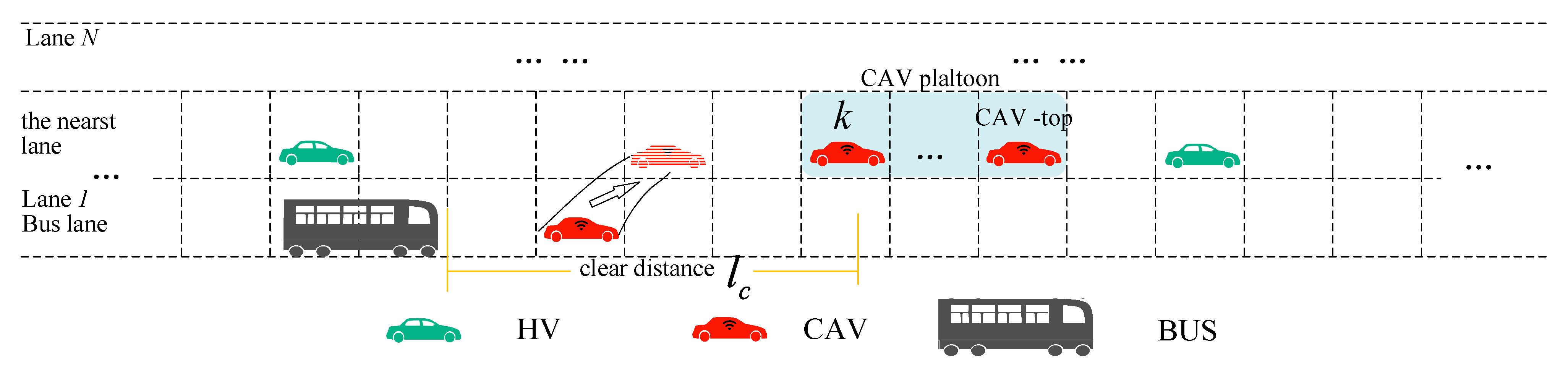
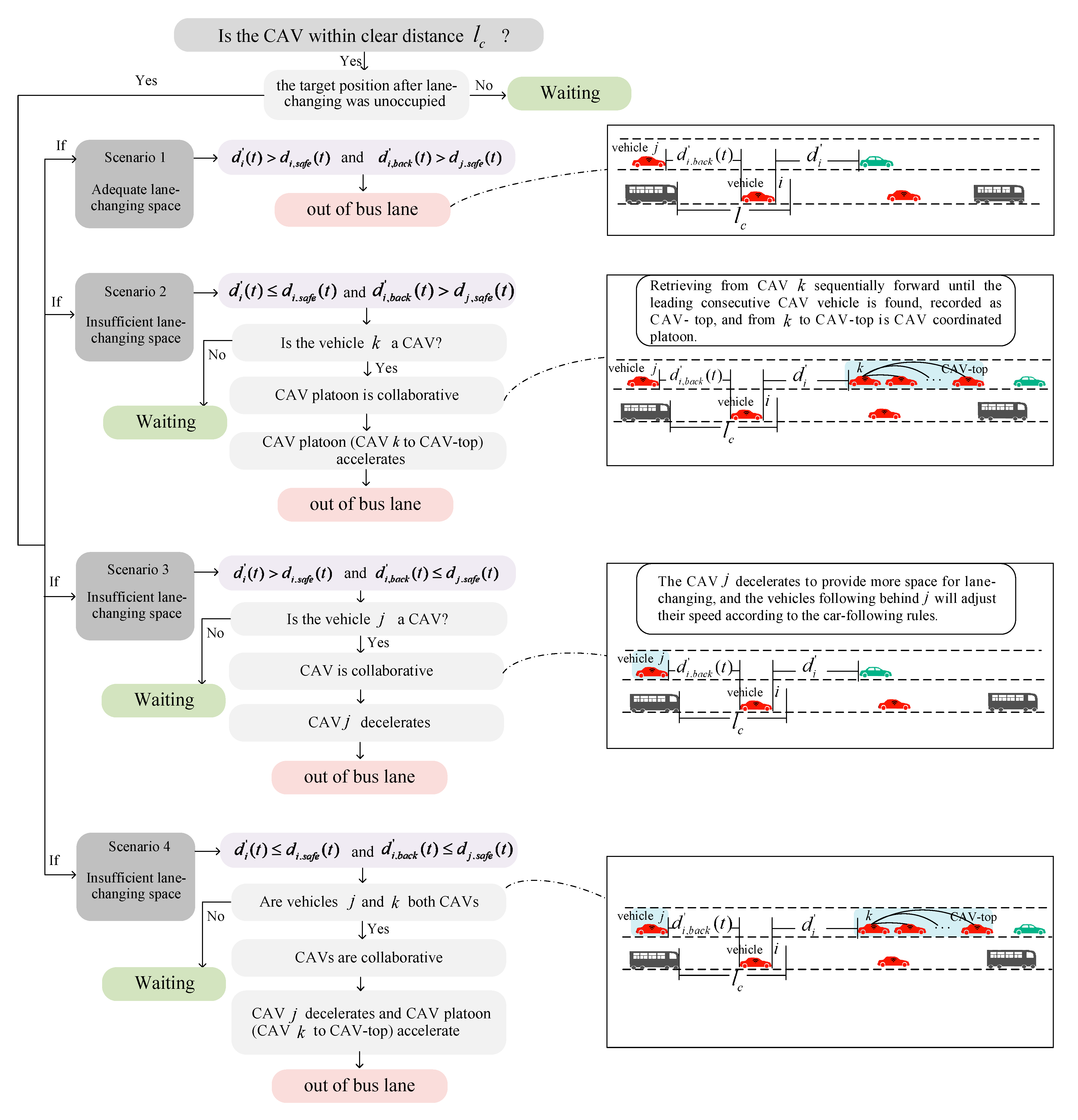
- In Section 3, we introduce a BLIP method based on the spatio-temporal clear distance (BLIP-ST) in Section 3.1 and establish the integrated heterogeneous traffic flow cellular automata model in Section 3.2. Then, we propose a CAVs borrowing bus lane control method considering the moving gap constraint in Section 3.3 and a CAV platoon collaborative lane-changing method in Section 3.4. When a target CAV that is within the clear distance of the bus cannot find the appropriate space to change lanes in time, the nearest CAV or CAV platoon on the adjacent lane will provide space by changing speeds.
- (3)
- The proposed models and method are validated through numerical simulations in Section 4.
- (4)
- We discuss the simulation results and compare the road operation performance before and after implementation across different strategies in Section 5.
- (5)
- We provide a conclusion in Section 6.
2. Assumptions and Notations
2.1. Assumptions
- (1)
- The traffic system consists of three vehicle types: HVs, CAVs, and human-driven buses, with each category exhibiting consistent performance parameters.
- (2)
- The scenario is confined to a road segment, ensuring that lane-changing behavior does not impact arrival at the destination. CAV borrowing and leaving behavior adhere to the instructions of the control center with a 100% obedience rate. Considering that the controlled CAV is between two buses and has a small range, the communication delay is not considered.
- (3)
- Leveraging V2X infrastructure, all connected and automated vehicles (CAVs) and the central control system maintain real-time awareness of surrounding traffic conditions.
- (4)
- Communication delays or losses are not explicitly considered.
2.2. Notations
3. CAV Control Strategy and Modeling
3.1. BLIP-ST
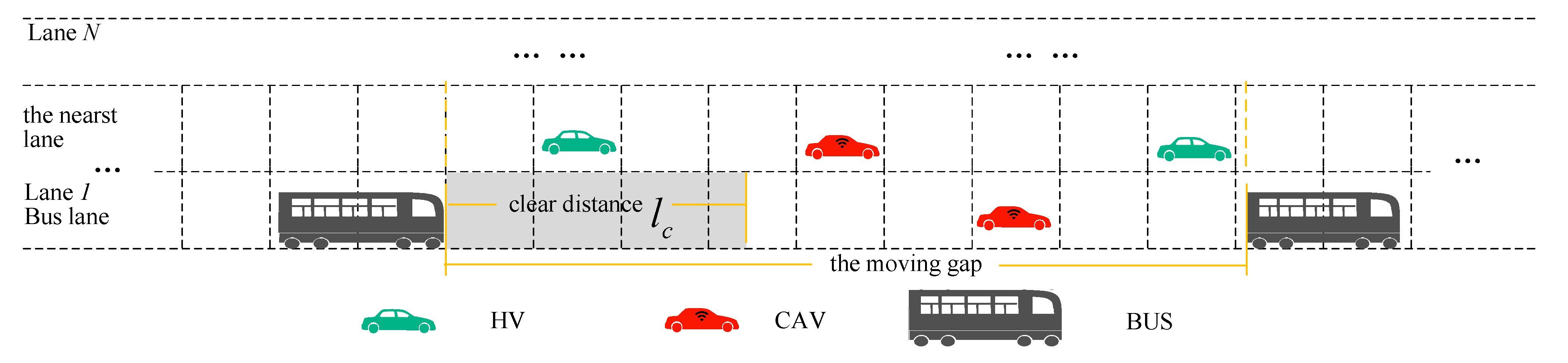
3.2. Modeling
3.3. CAVs’ Borrowing Bus Lane Control Method
3.4. CAVs Leaving Bus Lane Control Method
4. Numerical Simulations

| Location | Nature | Time | Average Flow |
|---|---|---|---|
| Yangtze River 1st Road, Yuzhong District, Chongqing | Urban two-lane section | 8:00–9:00 | 1800 veh/h |
5. Results and Discussion
5.1. Free Flow Situation
5.2. Congestion Situation
6. Conclusions
Author Contributions
Funding
Institutional Review Board Statement
Informed Consent Statement
Data Availability Statement
Conflicts of Interest
References
- Wu, D.; Deng, W.; Song, Y.; Wang, J.; Kong, D. Evaluating operational effects of bus lane with intermittent priority under connected vehicle environments. Discret. Dyn. Nat. Soc. 2017, 2017, 1659176. [Google Scholar] [CrossRef]
- Viegas, J.; Lu, B. Traffic control system with intermittent bus lanes. IFAC Proc. Vol. 1997, 30, 865–870. [Google Scholar] [CrossRef]
- Eichler, M.; Daganzo, C.F. Bus lanes with intermittent priority: Strategy formulae and an evaluation. Transp. Res. Part B Methodol. 2006, 40, 731–744. [Google Scholar] [CrossRef]
- Carey, G.; Bauer, T.; Giese, K. Bus Lane with Intermittent Priority (BLIMP) Concept Simulation Analysis; National Bus Rapid Transit Institute: Tampa, FL, USA, 2009. [Google Scholar]
- Xie, X.; Chiabaut, N.; Leclercq, L. Improving bus transit in cities with appropriate dynamic lane allocating strategies. Procedia-Soc. Behav. Sci. 2012, 48, 1472–1481. [Google Scholar] [CrossRef]
- Nicolas, C.; Xie, X.; Leclercq, L. Road capacity and travel times with bus lanes and intermittent priority activation: Analytical investigations. Transp. Res. Rec. 2012, 2315, 182–190. [Google Scholar]
- Wu, W.; Head, L.; Ma, W.; Yang, X. BLIP: Bus lanes with intermittent priority. In Proceedings of the Transportation Research Board 92nd Annual Meeting, Washington, DC, USA, 13–17 January 2013. [Google Scholar]
- Wu, W.; Head, L.; Yan, S.; Ma, W. Development and evaluation of bus lanes with intermittent and dynamic priority in connected vehicle environment. J. Intell. Transp. Syst. 2018, 22, 301–310. [Google Scholar] [CrossRef]
- Wu, D. A Study on the Capacity and Impact of Intermittent Priority Bus Lanes. Ph.D. Thesis, Southeast University, Nanjing, China, 2019. [Google Scholar]
- Ma, C.; Xu, X. Providing spatial-temporal priority control strategy for BRT lanes: A simulation approach. J. Transp. Eng. Part A Syst. 2020, 147, 385. [Google Scholar] [CrossRef]
- Chiabaut, N.; Barcet, A. Demonstration and evaluation of an intermittent bus lane strategy. Public Transp. 2019, 11, 443–456. [Google Scholar] [CrossRef]
- Chen, S.; Hu, L.; Yao, Z.; Zhu, B.; Jiang, Y. Efficient and environmentally friendly operation of intermittent dedicated lanes for connected autonomous vehicles in mixed traffic environments. Phys. A Stat. Mech. Appl. 2022, 608, 128310. [Google Scholar] [CrossRef]
- Wu, D.; Deng, W.; Song, Y.; Kong, D. Cellular Automaton Modeling of a Connected Vehicles-Based Bus Lane with Intermittent Priority. In Proceedings of the 16th COTA International Conference of Transportation Professionals, Shanghai, China, 6–9 July 2016; Transportation Research Board Institute of Transportation Engineers (ITE), American Society of Civil Engineers: Washington, DC, USA, 2016; pp. 735–746. [Google Scholar]
- Chen, X.; Lin, X.; He, F.; Li, M. Modeling and control of automated vehicle access on dedicated bus rapid transit lanes. Transp. Res. Part C 2020, 120, 102–123. [Google Scholar] [CrossRef]
- Pang, M.; Chai, Z.; Gong, D. Control of Connected and Automated Vehicles Driving on Dedicated Bus Lane Under Mixed Traffic. J. Transp. Syst. Eng. Inf. Technol. 2021, 21, 118–124. [Google Scholar]
- Dong, H.; Yang, J.; Quan, C. Dynamic Clearance Control Method for Reusing Bus Lanes under Vehicular Networking. J. Transp. Syst. Eng. Inf. Technol. 2024, 24, 12–20. [Google Scholar]
- Fakhrmoosavi, F.; Saedi, R.; Zockaie, A.; Talebpour, A. Impacts of Connected and Autonomous Vehicles on Traffic Flow with Heterogeneous Drivers Spatially Distributed over Large-Scale Networks. Transp. Res. Rec. 2020, 2674, 817–830. [Google Scholar] [CrossRef]
- Talebpour, A.; Mahmassani, H.S.; Hamdar, S.H. Modeling Lane-Changing Behavior in a Connected Environment: A Game Theory Approach. Transp. Res. Procedia 2015, 59, 216–232. [Google Scholar]
- Sala, M.; Soriguera, F. Capacity of a freeway lane with platoons of autonomous vehicles mixed with regular traffic. Transp. Res. Part B 2021, 147, 116–131. [Google Scholar] [CrossRef]
- Zhou, Y.J.; Zhu, H.B.; Guo, M.M.; Zhou, J.L. Impact of CACC vehicles’ cooperative driving strategy on mixed four-lane highway traffic flow. Phys. A Stat. Mech. Appl. 2020, 540, 122721. [Google Scholar] [CrossRef]
- Qin, Y. Research on the Analysis Method of Heterogeneous Traffic Flow Characteristics in Intelligent Connected Environment. Ph.D. Thesis, Southeast University, Nanjing, China, 2019. [Google Scholar]
- Liu, H.; Kan, X.; Shladover, S.E.; Lu, X.-Y.; Ferlis, R.E. Modeling impacts of cooperative adaptive cruise control on mixed traffic flow in multi-lane freeway facilities. Transp. Res. Part C Emerg. Technol. 2018, 95, 261–279. [Google Scholar] [CrossRef]
- Liang, J.; Geng, H.; Chen, L.; Yu, B.; Lu, G. Heterogeneous traffic flow model integrating bus and autonomous driving fleets. J. Southwest Jiaotong Univ. 2023, 58, 1090–1099. [Google Scholar]
- Shan, X.; Wan, C.; Hao, P.; Wu, G.; Barth, M.J. Developing A Novel Dynamic Bus Lane Control Strategy With Eco-Driving Under Partially Connected Vehicle Environment. IEEE Trans. Intell. Transp. Syst. 2024, 25, 5919–5934. [Google Scholar] [CrossRef]
- Yuan, Y.; Yuan, Y.; Yuan, B.; Li, X. Cooperative bus eco-approaching and lane-changing strategy in mixed connected and automated traffic environment. Transp. Res. Part C Emerg. Technol. 2024, 169, 104907. [Google Scholar] [CrossRef]
- Li, H.; Yuan, Z.; Yue, R.; Yang, G.; Chen, S.; Zhu, C. A lane usage strategy for general traffic access on bus lanes under partially connected vehicle environment. Transp. A Transp. Sci. 2025. [Google Scholar] [CrossRef]
- Liu, D.; Baldi, S.; Jain, V.; Yu, W.; Frasca, P. Cyclic Communication in Adaptive Strategies to Platooning: The Case of Synchronized Merging. IEEE Trans. Intell. Veh. 2021, 6, 490–500. [Google Scholar] [CrossRef]
- Zhao, C.; Dong, H.; Hao, W. Setting condition and traffic critical model for bus lane with time-division multiplexing. J. Zhejiang Univ. Eng. Sci. 2021, 55, 704–712. [Google Scholar]
- Jia, N.; Ma, S. Analytical Investigation of the Open Boundary Conditions in the Nagel-Schreckenberg Model. Phys. Rev. E 2009, 79, 031115. [Google Scholar] [CrossRef]
- Barlovic, R.; Huisinga, T.; Schadschneider, A.; Schreckenberg, M. Open boundaries in a cellular automaton model for traffic flow with metastable states. Phys. Rev. E 2002, 66, 046113. [Google Scholar] [CrossRef]
- Lu, H. Urban Traffic Management Evaluation System; China Communication Press: Beijing China, 2003. [Google Scholar]


| Notations | Description |
|---|---|
| Number of lanes. | |
| Clear distance of the bus at ; CAVs are forced to leave the bus lane within . | |
| Safe distance of vehicle at , including two parts: reaction distance and braking distance. | |
| The distance between vehicle and the preceding vehicle on the same lane at . | |
| The distance between vehicle and the preceding vehicle on the nearest lane at . | |
| The distance between vehicle and the following approaching vehicle on the nearest lane at . | |
| Acceleration, . | |
| Deceleration, , taking a negative value. | |
| The reaction time of the driver, , . | |
| The speed of vehicle at . | |
| The location of vehicle at . | |
| The location of the adjacent lane corresponding to the location of vehicle at . | |
| Maximum speed, . | |
| The cell state of . | |
| Unit of time. | |
| Randomization probability. | |
| Adaptive cruise control (ACC) following mode, CAV-HV or CAV-BUS; the value is 0 or 1. | |
| Human-driving car following mode, HV-HV, BUS-BUS, or HV-CAV; the value is 0 or 1. | |
| Cooperative Adaptive Cruise Control (CACC) following mode, CAV-CAV; the value is 0 or 1. | |
| Unit cell length. | |
| ,, | The length of HV, BUS, and CAV, respectively. |
| , | The quantity of vehicles in the bus lane in the moving gap and the quantity of vehicles in the adjacent lane in moving gap. |
| , | The average speed in the bus lane in the moving gap and the average speed in the adjacent lane in the moving gap. |
| Name | Variable | Value | Unit |
|---|---|---|---|
| the length of road | 2000 (2) | Cell (km) | |
| number of lanes | 2 | - | |
| time step | 1 | second (s) | |
| acceleration | , | 3, 5, 5 | m/s2 |
| deceleration | , , | −6, −8, −8 | m/s2 |
| The reaction time | , , | 0.4, 0.4, 0 | second (s) |
| The length of vehicle | , , , | 10, 5, 5 | cell (meters) |
| Maximum speed | , , | 14, 15, 15 | cell/s (m/s) |
| Random slowing probability | 0.2 | ||
| CAV penetration rate |
| Strategy | Explanation |
|---|---|
| BS | CAVs are allowed to use the bus lane. But the moving gap constraints are not considered. Additionally, CAV platoon collaborative lane changing is also not applied. |
| BS-MP | Based on BLIP-ST, the moving gap constraints are considered. CAV platoon collaborative lane changing is not applied, but single CAV collaborative lane changing is. |
| BS-CPC | Based on BLIP-ST, the moving gap constraints are considered, and CAV platoon collaborative lane changing is applied simultaneously. |
Disclaimer/Publisher’s Note: The statements, opinions and data contained in all publications are solely those of the individual author(s) and contributor(s) and not of MDPI and/or the editor(s). MDPI and/or the editor(s) disclaim responsibility for any injury to people or property resulting from any ideas, methods, instructions or products referred to in the content. |
© 2025 by the authors. Licensee MDPI, Basel, Switzerland. This article is an open access article distributed under the terms and conditions of the Creative Commons Attribution (CC BY) license (https://creativecommons.org/licenses/by/4.0/).
Share and Cite
Jiang, P.; Ma, X.; Li, Y. Analysis of Operational Effects of Bus Lanes with Intermittent Priority with Spatio-Temporal Clear Distance and CAV Platoon Coordinated Lane Changing in Intelligent Transportation Environment. Sensors 2025, 25, 2538. https://doi.org/10.3390/s25082538
Jiang P, Ma X, Li Y. Analysis of Operational Effects of Bus Lanes with Intermittent Priority with Spatio-Temporal Clear Distance and CAV Platoon Coordinated Lane Changing in Intelligent Transportation Environment. Sensors. 2025; 25(8):2538. https://doi.org/10.3390/s25082538
Chicago/Turabian StyleJiang, Pei, Xinlu Ma, and Yibo Li. 2025. "Analysis of Operational Effects of Bus Lanes with Intermittent Priority with Spatio-Temporal Clear Distance and CAV Platoon Coordinated Lane Changing in Intelligent Transportation Environment" Sensors 25, no. 8: 2538. https://doi.org/10.3390/s25082538
APA StyleJiang, P., Ma, X., & Li, Y. (2025). Analysis of Operational Effects of Bus Lanes with Intermittent Priority with Spatio-Temporal Clear Distance and CAV Platoon Coordinated Lane Changing in Intelligent Transportation Environment. Sensors, 25(8), 2538. https://doi.org/10.3390/s25082538