

A Deep Learning Model for 3D Ground Reaction Force Estimation Using Shoes with Three Uniaxial Load Cells


Abstract
1. Introduction
2. Materials and Methods
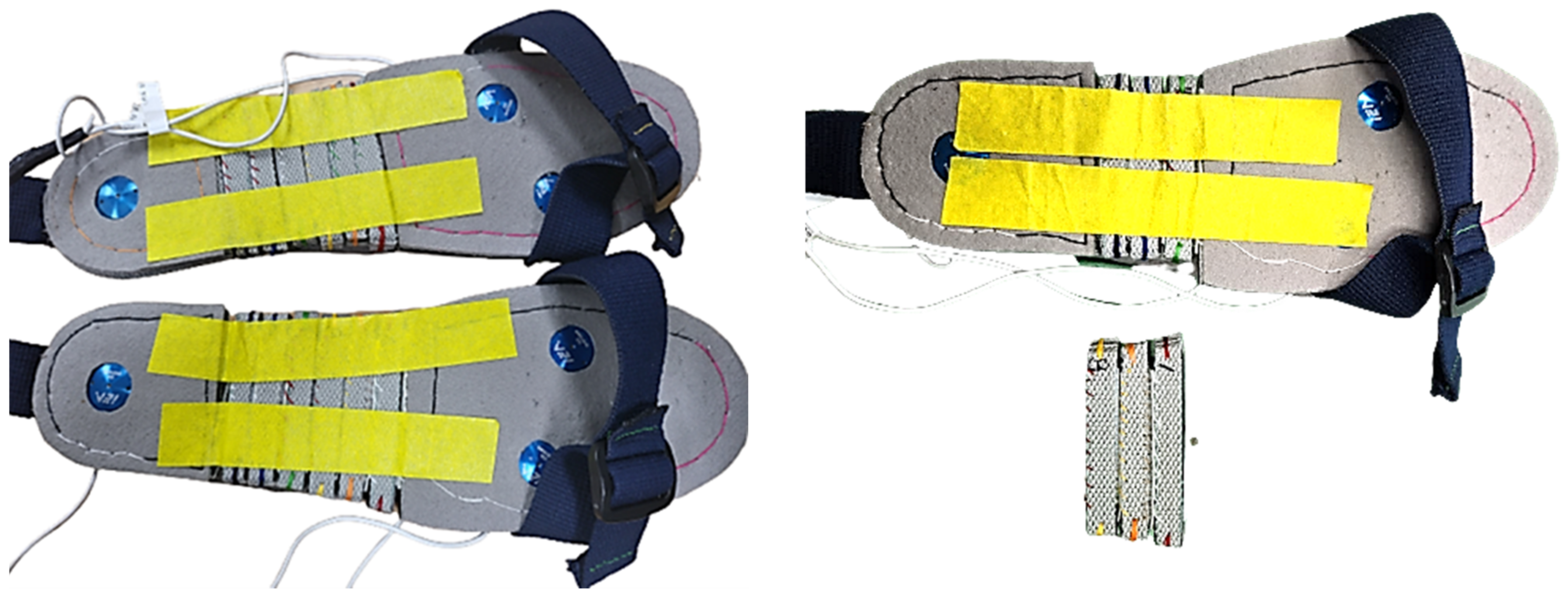
2.1. Shoe with Three Uniaxial Load Cells
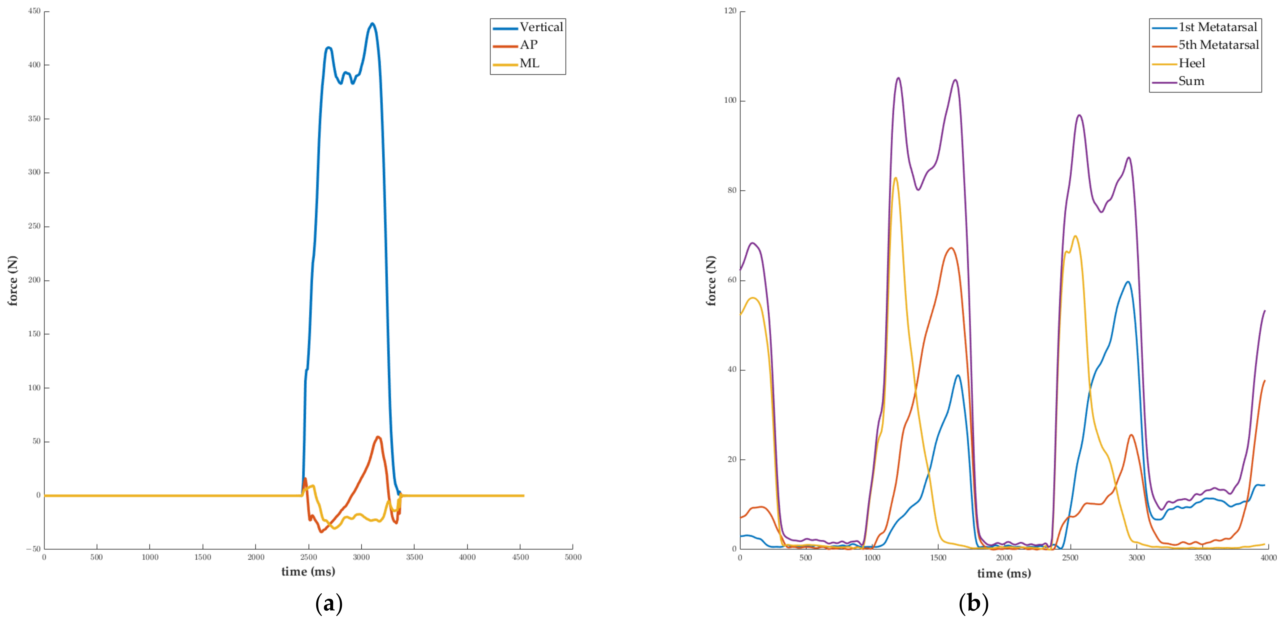
2.2. Experiment
2.3. Data Processing
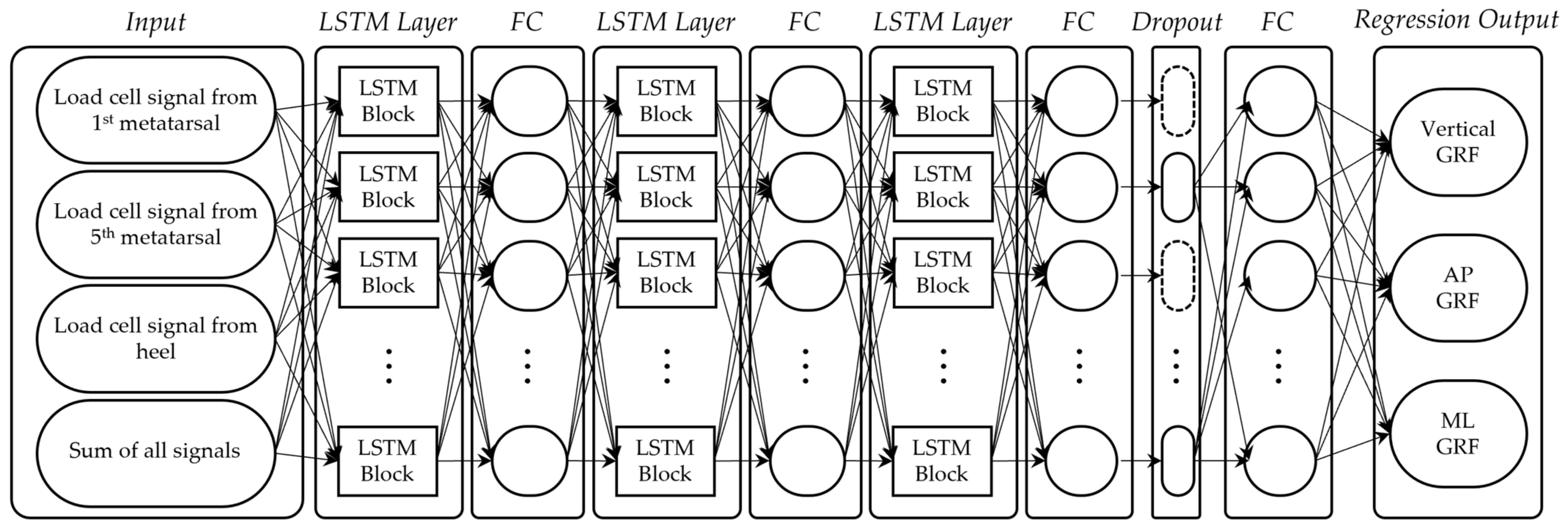
2.4. LSTM Seq2seq Layer
2.5. Validation
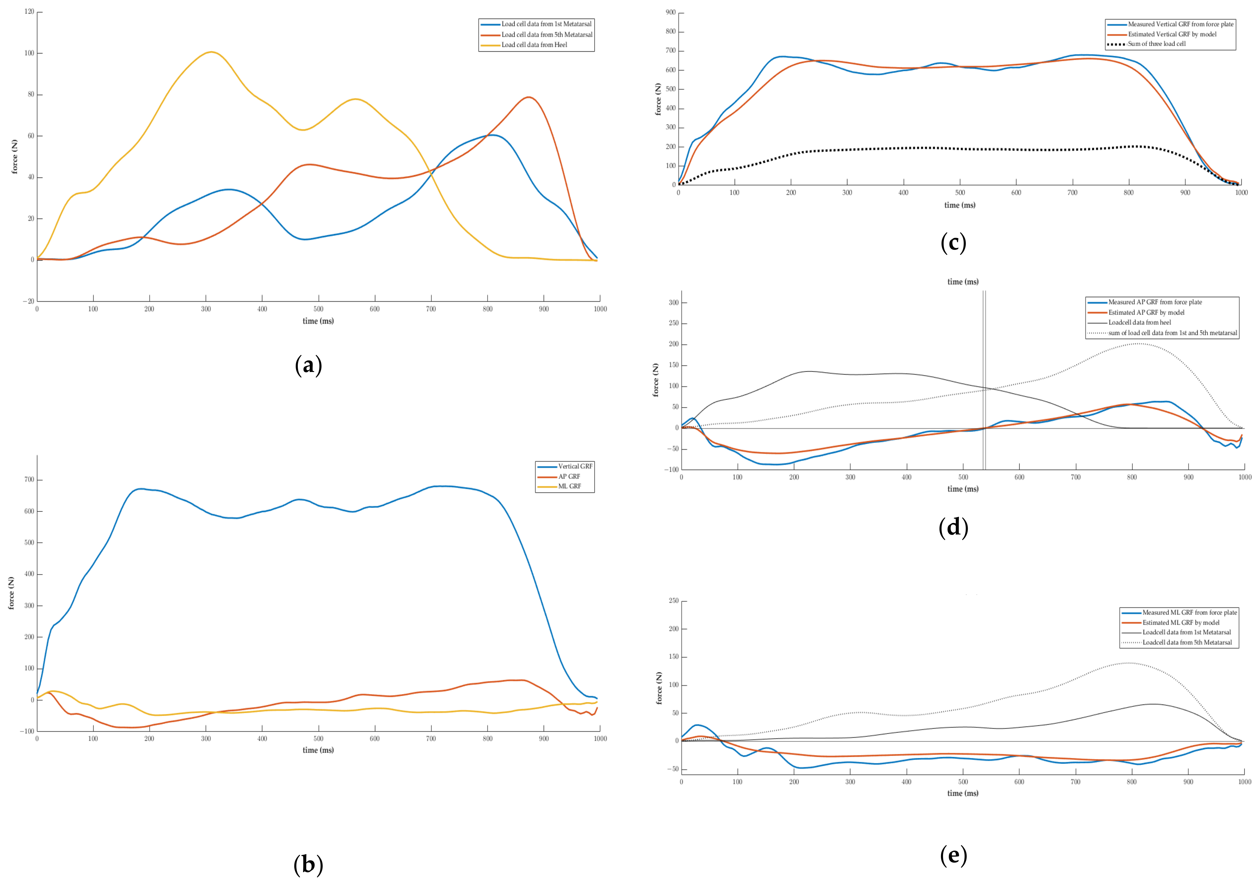
3. Results
4. Discussion
5. Conclusions
Supplementary Materials
Author Contributions
Funding
Institutional Review Board Statement
Informed Consent Statement
Data Availability Statement
Conflicts of Interest
References
- Baker, R.; Esquenazi, A.; Benedetti, M.G.; Desloovere, K. Gait Analysis: Clinical Facts. Eur. J. Phys. Rehabil. Med. 2016, 52, 560–574. [Google Scholar]
- Winter, D.A. Biomechanics and Motor Control of Human Gait, Normal, Elderly and Pathological; University of Waterloo Press: Waterloo, ON, Canada, 1991. [Google Scholar]
- CIR System Inc. Available online: https://www.gaitrite.com/ (accessed on 13 December 2022).
- XSENSOR Inc. Available online: https://www.xsensor.com/solutions-and-platform/human-performance/walkways-stance-pads/ (accessed on 8 February 2023).
- Tekscan Inc. Available online: https://www.tekscan.com (accessed on 8 December 2022).
- Bilney, B.; Morris, M.; Webster, K. Concurrent Related Validity of the GAITRite® Walkway System for Quantification of the Spatial and Temporal Parameters of Gait. Gait Posture 2003, 17, 68–74. [Google Scholar] [CrossRef] [PubMed]
- Vaillancourt, C. Physical Rehabilitation: Evidence-Based Examination, Evaluation, and Intervention. Phys. Ther. 2008, 88, 973. [Google Scholar] [CrossRef]
- Honert, E.C.; Hoitz, F.; Blades, S.; Nigg, S.R.; Nigg, B.M. Estimating Running Ground Reaction Forces from Plantar Pressure during Graded Running. Sensors 2022, 22, 3338. [Google Scholar] [CrossRef]
- Takayanagi, N.; Sudo, M.; Yamashiro, Y.; Lee, S.; Kobayashi, Y.; Niki, Y.; Shimada, H. Relationship between Daily and in-Laboratory Gait Speed among Healthy Community-Dwelling Older Adults. Sci. Rep. 2019, 9, 3496. [Google Scholar] [CrossRef] [PubMed]
- Foucher, K.C.; Thorp, L.E.; Orozco, D.; Hildebrand, M.; Wimmer, M.A. Differences in Preferred Walking Speeds in a Gait Laboratory Compared with the Real World after Total Hip Replacement. Arch. Phys. Med. Rehabil. 2010, 91, 1390–1395. [Google Scholar] [CrossRef]
- Pedar®: Dynamic Pressure Distribution inside the Footwear. Available online: https://www.novel.de/products/pedar/ (accessed on 11 January 2023).
- Savelberg, H.; De Lange, A. Assessment of the Horizontal, Fore-Aft Component of the Ground Reaction Force from Insole Pressure Patterns by using Artificial Neural Networks. Clin. Biomech. 1999, 14, 585–592. [Google Scholar] [CrossRef]
- Johnson, W.R.; Mian, A.; Robinson, M.A.; Verheul, J.; Lloyd, D.G.; Alderson, J.A. Multidimensional Ground Reaction Forces and Moments from Wearable Sensor Accelerations via Deep Learning. IEEE Trans. Biomed. Eng. 2020, 68, 289–297. [Google Scholar] [CrossRef]
- Choi, H.S.; Lee, C.H.; Shim, M.; Han, J.I.; Baek, Y.S. Design of an Artificial Neural Network Algorithm for a Low-Cost Insole Sensor to Estimate the Ground Reaction Force (GRF) and Calibrate the Center of Pressure (CoP). Sensors 2018, 18, 4349. [Google Scholar] [CrossRef]
- Oubre, B.; Lane, S.; Holmes, S.; Boyer, K.; Lee, S.I. Estimating Ground Reaction Force and Center of Pressure using Low-Cost Wearable Devices. IEEE Trans. Biomed. Eng. 2021, 69, 1461–1468. [Google Scholar] [CrossRef]
- Luo, Z.; Berglund, L.J.; An, K. Validation of F-Scan Pressure Sensor System: A Technical Note. J. Rehabil. Res. Dev. 1998, 35, 186. [Google Scholar]
- Rana, N.K. Application of Force Sensing Resistor (FSR) in Design of Pressure Scanning System for Plantar Pressure Measurement. In Proceedings of the 2009 Second International Conference on Computer and Electrical Engineering, Dubai, United Arab Emirates, 28–30 December 2009; Volume 2, pp. 678–685. [Google Scholar]
- Crea, S.; Donati, M.; De Rossi, S.M.M.; Oddo, C.M.; Vitiello, N. A Wireless Flexible Sensorized Insole for Gait Analysis. Sensors 2014, 14, 1073–1093. [Google Scholar] [CrossRef]
- Tao, W.; Zhang, J.; Li, G.; Liu, T.; Liu, F.; Yi, J.; Wang, H.; Inoue, Y. A Wearable Sensor System for Lower-Limb Rehabilitation Evaluation using the GRF and CoP Distributions. MST 2015, 27, 25701. [Google Scholar] [CrossRef]
- Giuseppe, Z. An Innovative Compact System to Measure Skiing Ground Reaction Forces and Flexural Angles of Alpine and Touring Ski Boots. Sensors 2023, 23, 836. [Google Scholar]
- Ardestani, M.M.; Chen, Z.; Wang, L.; Lian, Q.; Liu, Y.; He, J.; Li, D.; Jin, Z. Feed Forward Artificial Neural Network to Predict Contact Force at Medial Knee Joint: Application to Gait Modification. Neurocomputing 2014, 139, 114–129. [Google Scholar] [CrossRef]
- Bastien, G.J.; Gosseye, T.P.; Penta, M. A Robust Machine Learning Enabled Decomposition of Shear Ground Reaction Forces during the Double Contact Phase of Walking. Gait Posture 2019, 73, 221–227. [Google Scholar] [CrossRef]
- Sutskever, I.; Vinyals, O.; Le, Q.V. Sequence to Sequence Learning with Neural Networks. Adv. Neural Inf. Process. Syst. 2014, 27, 3104–3112. [Google Scholar]
- Seq2Seq Model in Machine Learning. Available online: https://www.geeksforgeeks.org/seq2seq-model-in-machine-learning/ (accessed on 3 January 2022).
- Rumelhart, D.E.; Hinton, G.E.; Williams, R.J. Learning Representations by Back-Propagating Errors. Nature 1986, 323, 533–536. [Google Scholar] [CrossRef]
- Elman, J.L. Finding Structure in Time. Cogn. Sci. 1990, 14, 179–211. [Google Scholar] [CrossRef]
- Noh, S. Analysis of Gradient Vanishing of RNNs and Performance Comparison. Information 2021, 12, 442. [Google Scholar] [CrossRef]
- Manaswi, N.K. Rnn and lstm. In Deep Learning with Applications Using Python; Springer: Berlin/Heidelberg, Germany, 2018; pp. 115–126. [Google Scholar]
- Sherstinsky, A. Fundamentals of Recurrent Neural Network (RNN) and Long Short-Term Memory (LSTM) Network. Phys. D 2020, 404, 132306. [Google Scholar] [CrossRef]
- Bland, J.M.; Altman, D. Statistical Methods for Assessing Agreement between Two Methods of Clinical Measurement. Lancet 1986, 327, 307–310. [Google Scholar] [CrossRef]
- i2A Systems Corp. Available online: https://i2asys.com/ (accessed on 1 December 2022).
- Morton, D.J. The Human Foot: Its Evolution, Physiology and Functional Disorders; Columbia University Press: New York, NY, USA, 1935. [Google Scholar]
- Soames, R.W. Foot Pressure Patterns during Gait. J. Biomed. Eng. 1985, 7, 120–126. [Google Scholar] [CrossRef] [PubMed]
- National Instruments Corp. Available online: https://ni.nubicom.co.kr/img/pdf/376047d.pdf (accessed on 3 January 2023).
- Liu, M.M.; Herzog, W.; Savelberg, H.H. Dynamic Muscle Force Predictions from EMG: An Artificial Neural Network Approach. J. Electromyogr. Kinesiol. 1999, 9, 391–400. [Google Scholar] [CrossRef] [PubMed]
- Fong, D.T.; Chan, Y.; Hong, Y.; Yung, P.S.; Fung, K.; Chan, K. Estimating the Complete Ground Reaction Forces with Pressure Insoles in Walking. J. Biomech. 2008, 41, 2597–2601. [Google Scholar] [CrossRef]
- Wei, F.; Crechiolo, A.; Haut, R.C. Prediction of Ground Reaction Forces in Level and Incline/Decline Walking from a Multistage Analysis of Plantar Pressure Data. J. Biomech. 2019, 84, 46–51. [Google Scholar] [CrossRef]
- Aqueveque, P.; Germany, E.; Osorio, R.; Pastene, F. Gait Segmentation Method using a Plantar Pressure Measurement System with Custom-made Capacitive Sensors. Sensors 2020, 20, 656. [Google Scholar] [CrossRef]
- Whittle, M.W. Gait Analysis: An Introduction; Heinemann, B., Ed.; University of Oxford: Oxford, UK, 2014. [Google Scholar]
- Kim, K. Implementation of Gait Pattern Monitoring System using FSR (Force Sensitive Resistor) Sensor. J. Semicond. Disp. Technol. 2021, 20, 56–60. [Google Scholar]
- Perry, J. Gait Analysis. Normal and Pathological Function; Slack: San Francisco, CA, USA, 2010; pp. 19–47. [Google Scholar]
- Koltermann, J.J.; Gerber, M.; Beck, H.; Beck, M. Validation of the HUMAC Balance System in Comparison with Conventional Force Plates. Technologies 2017, 5, 44. [Google Scholar] [CrossRef]
- Hausdorff, J.M.; Rios, D.A.; Edelberg, H.K. Gait Variability and Fall Risk in Community-Living Older Adults: A 1-Year Prospective Study. Arch. Phys. Med. Rehabil. 2001, 82, 1050–1056. [Google Scholar] [CrossRef]
- Olivier, B.; Cédric, A.; Callisaya, M.L.; De Cock, A.; Helbostad, J.L.; Kressig, R.W.; Srikanth, V.; Steinmetz, J.; Blumen, H.M.; Joe, V.; et al. Poor Gait Performance and Prediction of Dementia: Results from a Meta-Analysis. J. Am. Med. Dir. Assoc. 2016, 17, 482–490. [Google Scholar]
- Olney, S.J.; Richards, C. Hemiparetic Gait Following Stroke. Part I: Characteristics. Gait Posture 1996, 4, 136–148. [Google Scholar] [CrossRef]


| Characteristic | Value |
|---|---|
| Capacity | 980.70 N |
| Linearity | 1.00% |
| Output | 5.0 V |
| Tolerance | 14,700.00 N |
| Voltage/force coefficient | 441.00~637.00 N/voltage |
| Weight | 27.10 g (with 1.0 m shield wire) |
| Dimension | Radius: 30.00 mm, height: 6.90 mm |
| Material | Aluminum |
| Result | Axis | Value |
|---|---|---|
| Correlation coefficient | Vertical | 0.97 |
| AP | 0.96 | |
| ML | 0.90 | |
| RMSE (N) | Vertical | 65.12 |
| AP | 15.50 | |
| ML | 9.83 | |
| Mid-stance timing error (abs) | 0.06 s | |
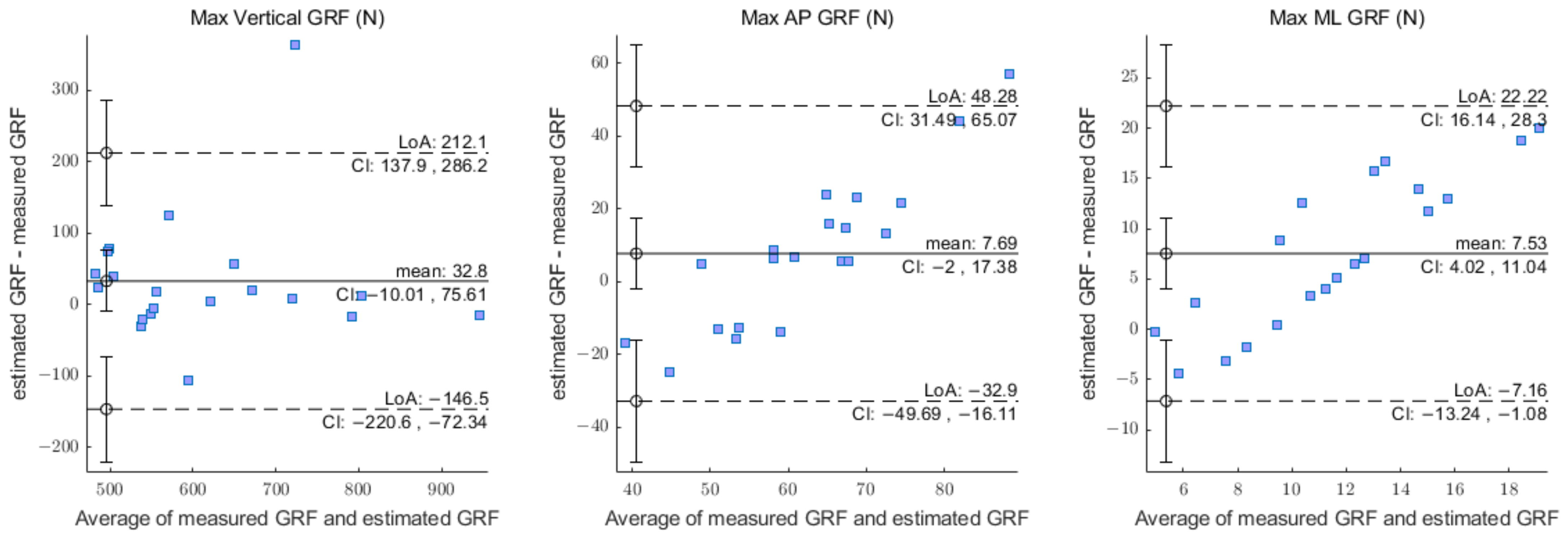
| Variables | LLoA, ULoA (N) | LoA 95% CI (N) | Mean Difference 95% CI (N) |
|---|---|---|---|
| Max vertical | −146.50, 212.10 | −220.70, 286.20 | −10.02, 75.61 |
| Max AP | −32.90, 48.28 | −49.69, 65.06 | −2.00, 17.38 |
| Max ML | −7.16, 22.22 | −13.24, 28.30 | 4.03, 11.04 |
| Result | Axis | Value | |
|---|---|---|---|
| Group with Similar Timing | Group with Different Timing | ||
| n | 5 | 15 | |
| Correlation coefficient | Vertical | 0.96 | 0.98 |
| AP | 0.94 | 0.96 | |
| ML | 0.82 | 0.92 | |
| RMSE (N) | Vertical | 99.25 | 53.73 |
| AP | 16.71 | 15.09 | |
| ML | 11.27 | 9.35 | |
Disclaimer/Publisher’s Note: The statements, opinions and data contained in all publications are solely those of the individual author(s) and contributor(s) and not of MDPI and/or the editor(s). MDPI and/or the editor(s) disclaim responsibility for any injury to people or property resulting from any ideas, methods, instructions or products referred to in the content. |
© 2023 by the authors. Licensee MDPI, Basel, Switzerland. This article is an open access article distributed under the terms and conditions of the Creative Commons Attribution (CC BY) license (https://creativecommons.org/licenses/by/4.0/).
Share and Cite
Kim, J.; Kang, H.; Lee, S.; Choi, J.; Tack, G. A Deep Learning Model for 3D Ground Reaction Force Estimation Using Shoes with Three Uniaxial Load Cells. Sensors 2023, 23, 3428. https://doi.org/10.3390/s23073428
Kim J, Kang H, Lee S, Choi J, Tack G. A Deep Learning Model for 3D Ground Reaction Force Estimation Using Shoes with Three Uniaxial Load Cells. Sensors. 2023; 23(7):3428. https://doi.org/10.3390/s23073428
Chicago/Turabian StyleKim, Junggil, Hyeon Kang, Seulgi Lee, Jinseung Choi, and Gyerae Tack. 2023. "A Deep Learning Model for 3D Ground Reaction Force Estimation Using Shoes with Three Uniaxial Load Cells" Sensors 23, no. 7: 3428. https://doi.org/10.3390/s23073428
APA StyleKim, J., Kang, H., Lee, S., Choi, J., & Tack, G. (2023). A Deep Learning Model for 3D Ground Reaction Force Estimation Using Shoes with Three Uniaxial Load Cells. Sensors, 23(7), 3428. https://doi.org/10.3390/s23073428