
SBAS-InSAR Based Deformation Monitoring of Tailings Dam: The Case Study of the Dexing Copper Mine No.4 Tailings Dam

Abstract
:1. Introduction
2. Study Area
3. Materials and Methods
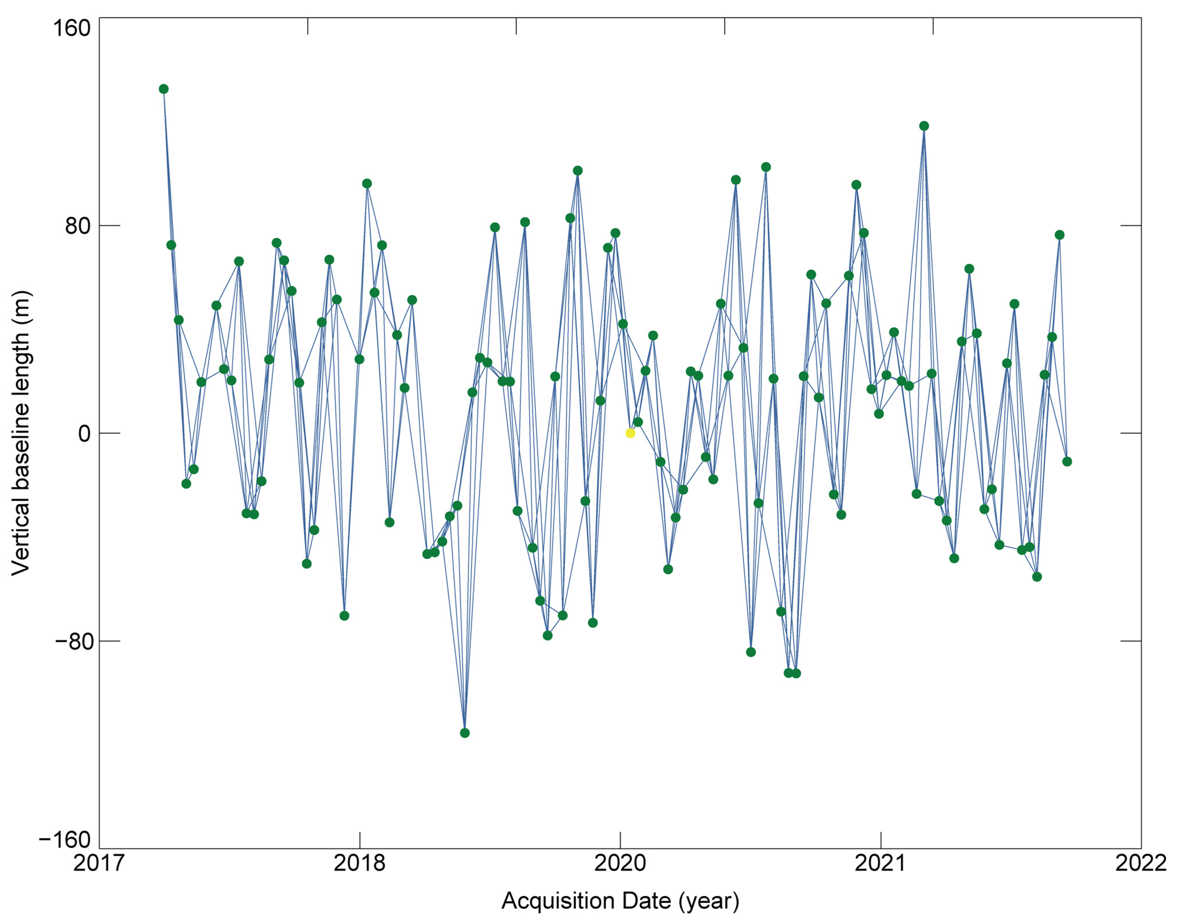
3.1. Data
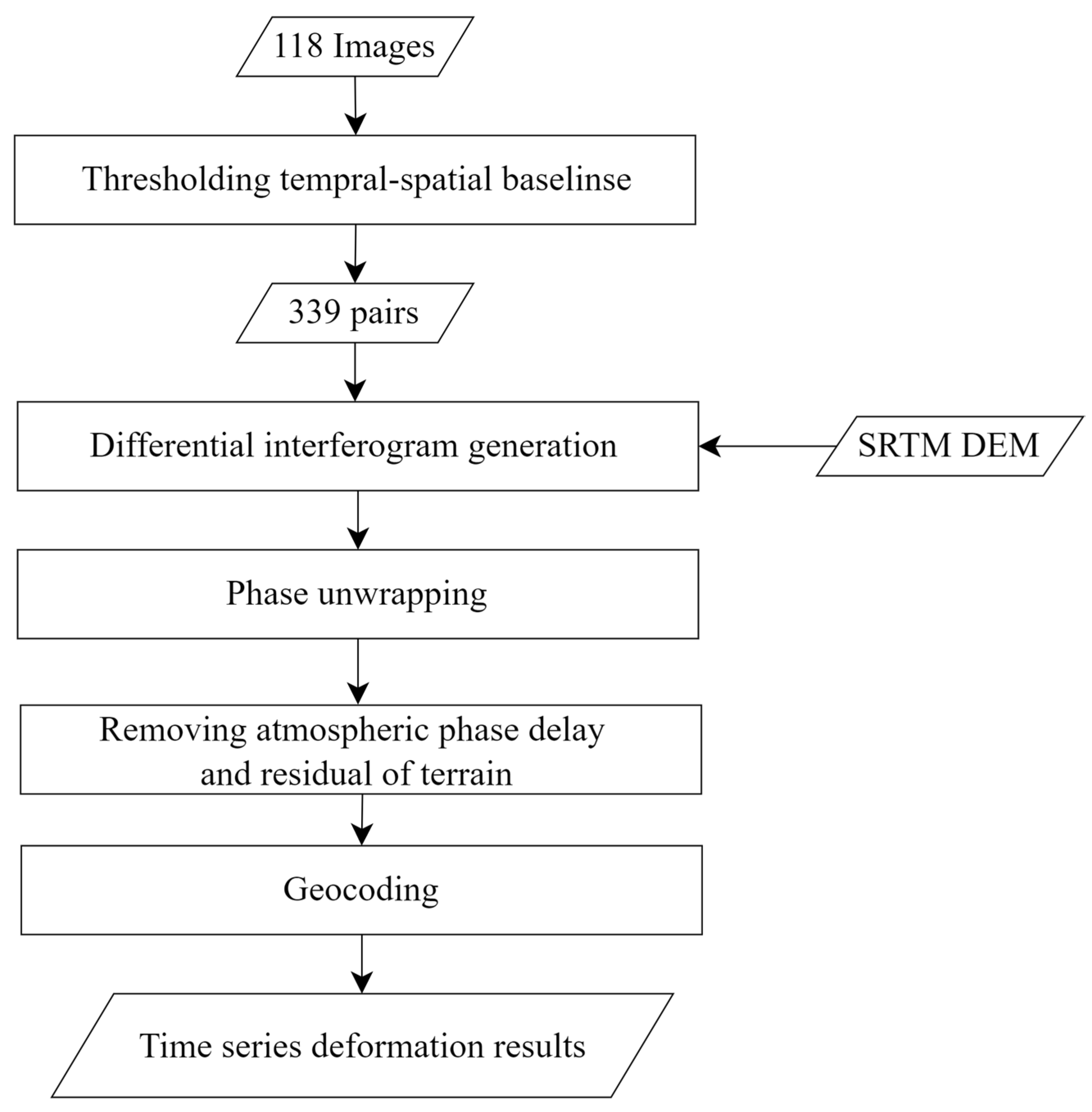
3.2. Methodology
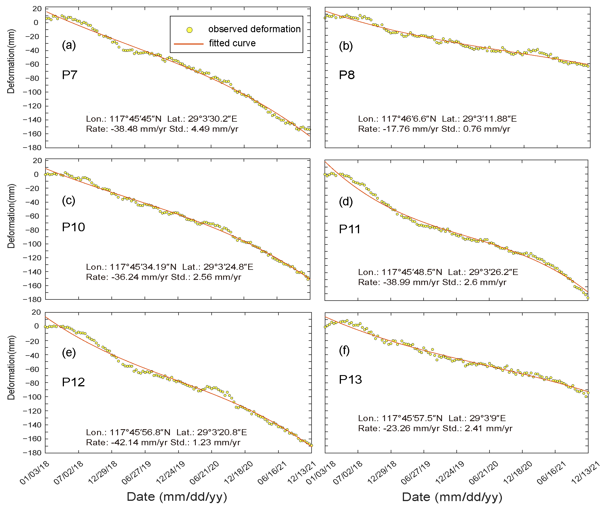
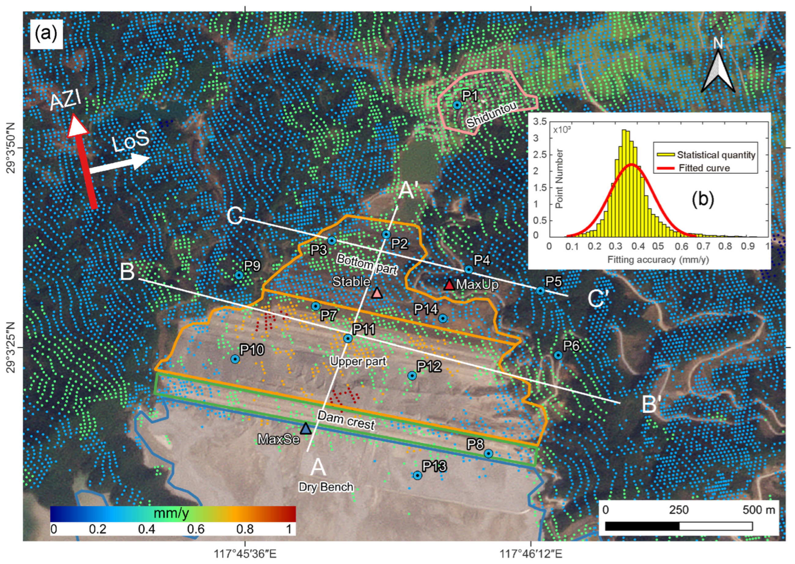
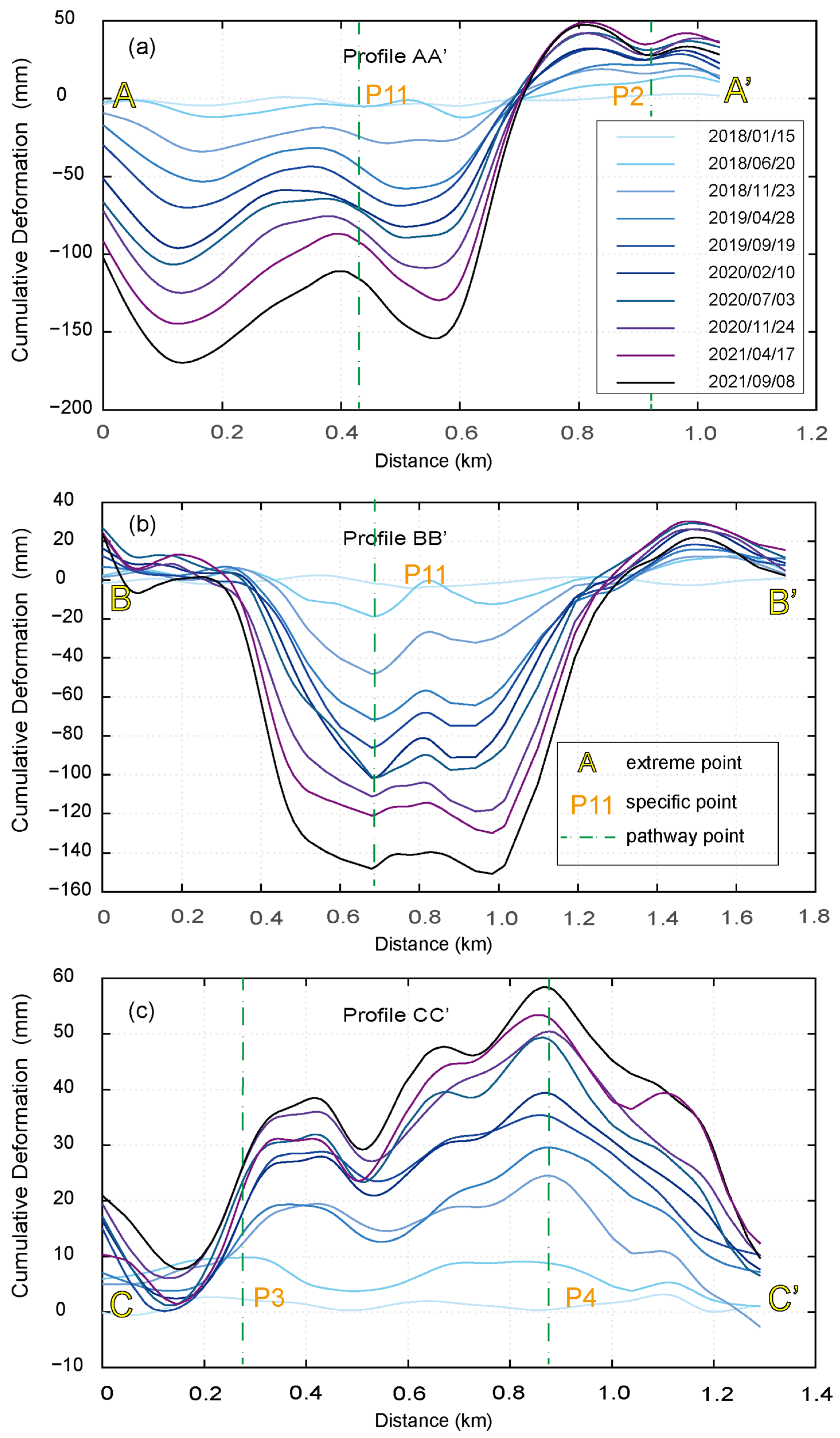
4. Result
5. Discussion
5.1. Precision Checking and Impact of Errors
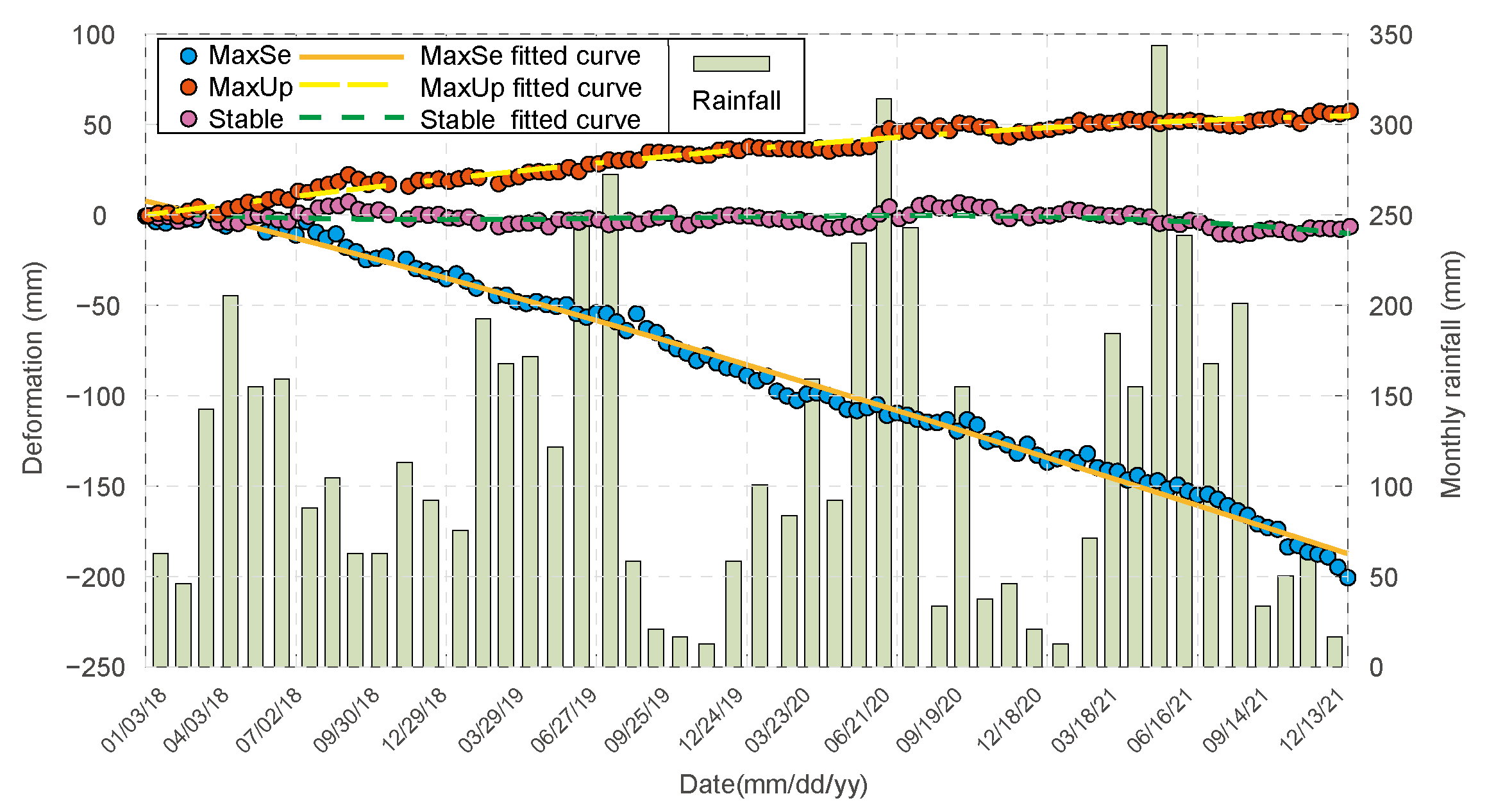
5.2. Cause Analysis of the Deformation in Dexing No.4 Tailings Dam
- The drainage system of the tailings pond and tailings dam has played a role in timely evacuation of surface water, and the underground drainage and seepage pipes are also in normal operation, so there is no excess water storage in the tailings pond;
- The catchment area of the tailings reservoir is small, so the amount of water brought by rainfall is small, and it is difficult to have a significant impact on the tailings dam.
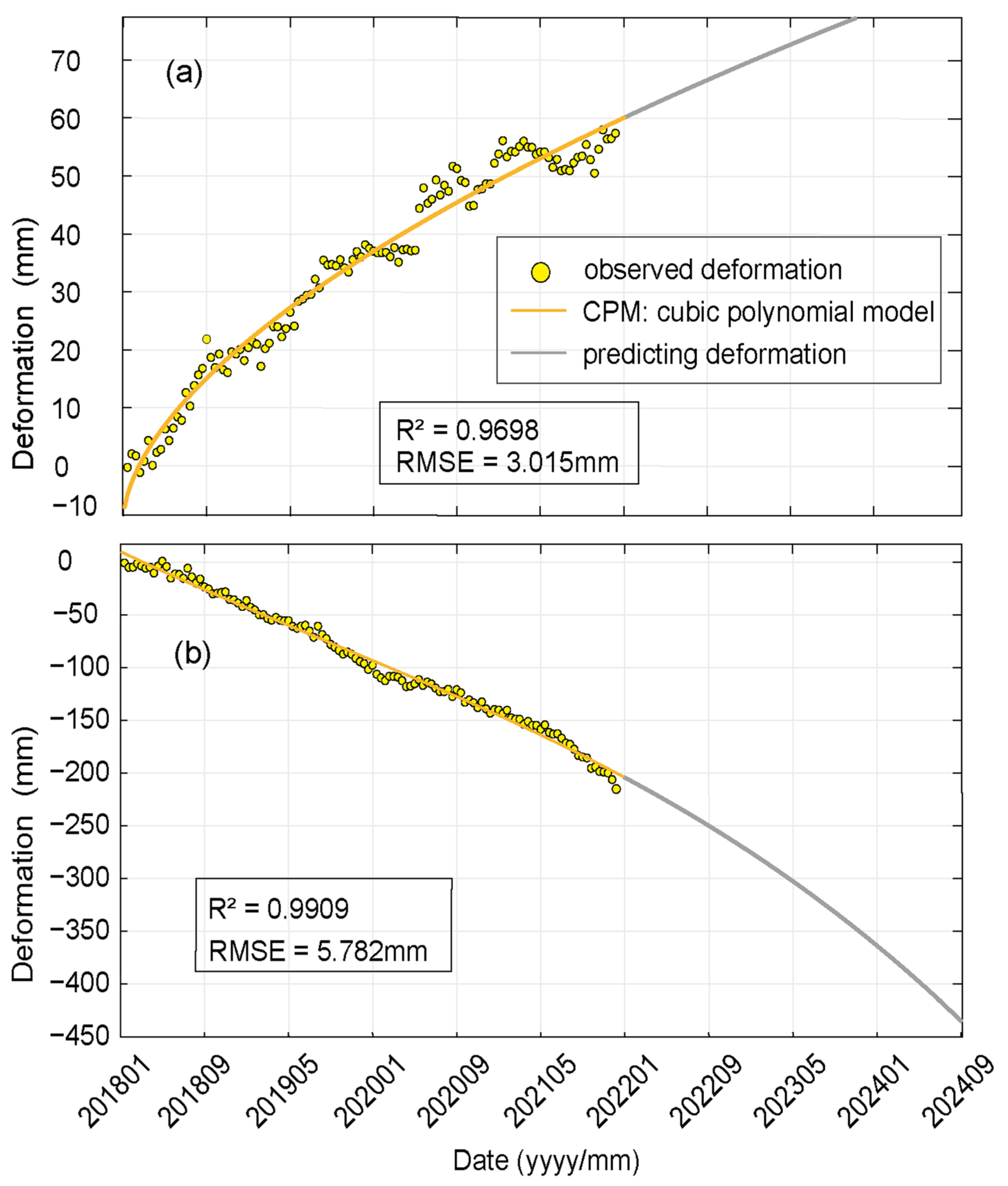
5.3. Deformation Trend and Prediction
6. Conclusions
Author Contributions
Funding
Institutional Review Board Statement
Informed Consent Statement
Data Availability Statement
Conflicts of Interest
References
- Hudson-Edwards, K. Tackling mine wastes. Science 2016, 352, 288–290. [Google Scholar] [CrossRef]
- U.S. Environmental Protection Agency. Technical Report: Design and Evaluation of Tailing Dams; U.S. Environmental Protection Agency: Washington, DC, USA, 1994; Chapter 4; pp. 25–30. Available online: https://archive.epa.gov/epawaste/nonhaz/industrial/special/web/pdf/tailings.pdf (accessed on 14 June 2023).
- ICOLD (International Commission On Large Dams). Tailings Dams Risks of Dangerous Occurrences—Lessons Learned from Practical Experiences; Commission Internationale des Grand Barrages: Paris, France, 2001; p. 121. [Google Scholar]
- WISE (World Information Service on Energy). Chronology of Major Tailings Dam Failures (From 1960 to 2023). WISE Uranium Project, Tailings Dam Safety. 2023. Available online: http://www.wise-uranium.org/mdaf.html (accessed on 14 June 2023).
- Grebby, S.; Sowter, A.; Gluyas, J.; Toll, D.; Gee, D.; Athab, A.; Girindran, R. Advanced analysis of satellite data reveals ground deformation precursors to the Brumadinho Tailings Dam collapse. Commun. Earth Environ. 2021, 2, 2. [Google Scholar] [CrossRef]
- MINING.COM. Tailings Pond Collapse Affects World’s Highest Human Settlement. 2021. Available online: https://www.mining.com/tailings-pond-collapse-affects-worlds-highest-human-settlement/ (accessed on 14 June 2023).
- Duan, H.; Li, Y.; Jiang, H.; Li, Q.; Jiang, W.; Tian, Y.; Zhang, J. Retrospective monitoring of slope failure event of tailings dam using InSAR time-series observations. Nat. Hazards 2023, 117, 2375–2391. [Google Scholar] [CrossRef]
- Wei, Z.; Yin, G.; Wan, L.; Li, G. A case study on a geotechnical investigation of drainage methods for heightening a tailings dam. Environ. Earth Sci. 2016, 75, 106. [Google Scholar] [CrossRef]
- Du, Z.; Ge, L.; Ng, A.H.-M.; Zhu, Q.; Horgan, F.G.; Zhang, Q. Risk assessment for tailings dams in Brumadinho of Brazil using InSAR time series approach. Sci. Total Environ. 2020, 717, 137125. [Google Scholar] [CrossRef]
- Wu, M.; Ye, Y.; Hu, N.; Wang, Q.; Tan, W. Scientometric analysis on the review research evolution of tailings dam failure disasters. Environ. Sci. Pollut. Res. 2022, 30, 13945–13959. [Google Scholar] [CrossRef]
- Canadian Broadcasting Corporation; Paige, P. Canada Opens Formal Investigation into Imperial’s Oilsands Tailings Leak in Northern Alberta|CBC News. Available online: https://www.cbc.ca/news/canada/edmonton/canada-opens-formal-investigation-into-imperial-s-oilsands-tailings-leak-in-northern-alberta-1.6832386 (accessed on 24 November 2023).
- Cacciuttolo, C.; Cano, D. Spatial and Temporal Study of Supernatant Process Water Pond in Tailings Storage Facilities: Use of Remote Sensing Techniques for Preventing Mine Tailings Dam Failures. Sustainability 2023, 15, 4984. [Google Scholar] [CrossRef]
- Valentina, R.L. Bolivian Authorities Investigate Tailings Pond Collapse near Potosí. Available online: https://www.mining.com/bolivian-authorities-investigate-tailings-pond-collapse-near-potosi/ (accessed on 24 November 2023).
- Petley, D. Thelkoloi: Another Tailings Failure, This Time in India—The Landslide Blog—AGU Blogosphere. Available online: https://blogs.agu.org/landslideblog/2022/01/24/thelkoloi/ (accessed on 24 November 2023).
- Petley, D. Pau Branco: Another Significant Mining-Related Landslide in Brazil. Available online: https://blogs.agu.org/landslideblog/2022/01/11/pau-branco-1/ (accessed on 24 November 2023).
- Petley, D. Ananea: A Significant Mine Waste Failure in Peru. Available online: https://blogs.agu.org/landslideblog/2021/11/30/ananea-1/ (accessed on 24 November 2023).
- Sentinel Vision Team. The Largest Angolan Diamond Mine Poisons Kasai River, DRC. Available online: https://www.sentinelvision.eu/gallery/html/59f7f8cfa0ef49bab141c4eb6f55aee4 (accessed on 24 November 2023).
- Ruppen, D.; Runnalls, J.; Tshimanga, R.M.; Wehrli, B.; Odermatt, D. Optical Remote Sensing of Large-Scale Water Pollution in Angola and DR Congo Caused by the Catoca Mine Tailings Spill. Int. J. Appl. Earth Obs. Geoinf. 2023, 118, 103237. [Google Scholar] [CrossRef]
- Lin, Y.N.; Park, E.; Wang, Y.; Quek, Y.P.; Lim, J.; Alcantara, E.; Loc, H.H. The 2020 Hpakant Jade Mine Disaster, Myanmar: A Multi-Sensor Investigation for Slope Failure. ISPRS J. Photogramm. Remote Sens. 2021, 177, 291–305. [Google Scholar] [CrossRef]
- Zhao, H.; Yang, Z.; Zhang, H.; Meng, J.; Jin, Q.; Ming, S. Emergency Monitoring of a Tailings Pond Leakage Accident Based on the GEE Platform. Sustainability 2022, 14, 8558. [Google Scholar] [CrossRef]
- Delgado, A.; Gil, F.; Chullunquía, J.; Valdivia, T.; Carbajal, C. Water Quality Analysis in Mantaro River, Peru, Before and After the Tailing’s Accident Using the Grey Clustering Method. Int. J. Adv. Sci. Eng. Inf. Technol. 2021, 11, 917. [Google Scholar] [CrossRef]
- Petley, D. Hindalco, Muri: Another Tailings Failure, This Time in India. Available online: https://blogs.agu.org/landslideblog/2019/04/13/hindalco-tailings-1/ (accessed on 24 November 2023).
- Silva Rotta, L.H.; Alcântara, E.; Park, E.; Negri, R.G.; Lin, Y.N.; Bernardo, N.; Mendes, T.S.G.; Souza Filho, C.R. The 2019 Brumadinho Tailings Dam Collapse: Possible Cause and Impacts of the Worst Human and Environmental Disaster in Brazil. Int. J. Appl. Earth Obs. Geoinf. 2020, 90, 102119. [Google Scholar] [CrossRef]
- Petley, D. Cobriza, Peru: Another Significant Tailings Dam Failure—The Landslide Blog—AGU Blogosphere. Available online: https://blogs.agu.org/landslideblog/2019/07/16/cobriza-mine-1/ (accessed on 24 November 2023).
- Xie, L.; Xu, W.; Ding, X.; Bürgmann, R.; Giri, S.; Liu, X. A multi-platform, open-source, and quantitative remote sensing framework for dam-related hazard investigation: Insights into the 2020 Sardoba dam collapse. Int. J. Appl. Earth Obs. Geoinf. 2022, 111, 102849. [Google Scholar] [CrossRef]
- Gama, F.F.; Paradella, W.R.; Mura, J.C.; De Oliveira, C.G. Advanced DINSAR analysis on dam stability monitoring: A case study in the Germano mining complex (Mariana, Brazil) with SBAS and PSI techniques. Remote Sens. Appl. Soc. Environ. 2019, 16, 100267. [Google Scholar] [CrossRef]
- Paradella, W.R.; Ferretti, A.; Mura, J.C.; Colombo, D.; Gama, F.F.; Tamburini, A.; Santos, A.R.; Novali, F.; Galo, M.; Camargo, P.O.; et al. Mapping surface deformation in open pit iron mines of Carajás Province (Amazon Region) using an integrated SAR analysis. Eng. Geol. 2015, 193, 61–78. [Google Scholar] [CrossRef]
- Mura, J.; Gama, F.; Paradella, W.; Negrão, P.; Carneiro, S.; De Oliveira, C.; Brandão, W. Monitoring the Vulnerability of the Dam and Dikes in Germano Iron Mining Area after the Collapse of the Tailings Dam of Fundão (Mariana-MG, Brazil) Using DInSAR Techniques with TerraSAR-X Data. Remote Sens. 2018, 10, 1507. [Google Scholar] [CrossRef]
- Mura, J.; Paradella, W.; Gama, F.; Silva, G.; Galo, M.; Camargo, P.; Silva, A.; Silva, A. Monitoring of Non-Linear Ground Movement in an Open Pit Iron Mine Based on an Integration of Advanced DInSAR Techniques Using TerraSAR-X Data. Remote Sens. 2016, 8, 409. [Google Scholar] [CrossRef]
- Gama, F.F.; Mura, J.C.; Paradella, W.R.; De Oliveira, C.G. Deformations Prior to the Brumadinho Dam Collapse Revealed by Sentinel-1 InSAR Data Using SBAS and PSI Techniques. Remote Sens. 2020, 12, 3664. [Google Scholar] [CrossRef]
- Marchamalo-Sacristán, M.; Ruiz-Armenteros, A.M.; Lamas-Fernández, F.; González-Rodrigo, B.; Martínez-Marín, R.; Delgado-Blasco, J.M.; Bakon, M.; Lazecky, M.; Perissin, D.; Papco, J.; et al. MT-InSAR and Dam Modeling for the Comprehensive Monitoring of an Earth-Fill Dam: The Case of the Benínar Dam (Almería, Spain). Remote Sens. 2023, 15, 2802. [Google Scholar] [CrossRef]
- Necsoiu, M.; Walter, G.R. Detection of uranium mill tailings settlement using satellite-based radar interferometry. Eng. Geol. 2015, 197, 267–277. [Google Scholar] [CrossRef]
- Wang, H.; Li, K.; Zhang, J.; Hong, L.; Chi, H. Monitoring and Analysis of Ground Surface Settlement in Mining Clusters by SBAS-InSAR Technology. Sensors 2022, 22, 3711. [Google Scholar] [CrossRef]
- Hu, X.; Oommen, T.; Lu, Z.; Wang, T.; Kim, J.-W. Consolidation settlement of Salt Lake County tailings impoundment revealed by time-series InSAR observations from multiple radar satellites. Remote Sens. Environ. 2017, 202, 199–209. [Google Scholar] [CrossRef]
- Gabriel, A.K.; Goldstein, R.M.; Zebker, H.A. Mapping small elevation changes over large areas: Differential radar interferometry. J. Geophys. Res. 1989, 94, 9183. [Google Scholar] [CrossRef]
- Wang, J.; Liang, Z.; Han, P.; Li, G.; Chen, F.; Liu, B. Analysis of the characteristics and causations of surface deformation based on TS-InSAR: A case study of Jimo district, China. Environ. Sci. Pollut. Res. 2023, 30, 40049–40061. [Google Scholar] [CrossRef]
- Wang, S.; Zhang, G.; Chen, Z.; Cui, H.; Zheng, Y.; Xu, Z.; Li, Q. Surface deformation extraction from small baseline subset synthetic aperture radar interferometry (SBAS-InSAR) using coherence-optimized baseline combinations. GISci. Remote Sens. 2022, 59, 295–309. [Google Scholar] [CrossRef]
- Wright, T.J. Toward mapping surface deformation in three dimensions using InSAR. Geophys. Res. Lett. 2004, 31, L01607. [Google Scholar] [CrossRef]
- Aswathi, J.; Binoj Kumar, R.B.; Oommen, T.; Bouali, E.H.; Sajinkumar, K.S. InSAR as a tool for monitoring hydropower projects: A review. Energy Geosci. 2022, 3, 160–171. [Google Scholar] [CrossRef]
- Chen, Y.; Tong, Y.; Tan, K. Coal Mining Deformation Monitoring Using SBAS-InSAR and Offset Tracking: A Case Study of Yu County, China. IEEE J. Sel. Top. Appl. Earth Obs. Remote Sens. 2020, 13, 6077–6087. [Google Scholar] [CrossRef]
- Liu, Y.; Fan, H.; Wang, L.; Zhuang, H. Monitoring of surface deformation in a low coherence area using distributed scatterers InSAR: Case study in the Xiaolangdi Basin of the Yellow River, China. Bull. Eng. Geol. Environ. 2021, 80, 25–39. [Google Scholar] [CrossRef]
- Pang, Z.; Jin, Q.; Fan, P.; Jiang, W.; Lv, J.; Zhang, P.; Cui, X.; Zhao, C.; Zhang, Z. Deformation Monitoring and Analysis of Reservoir Dams Based on SBAS-InSAR Technology—Banqiao Reservoir. Remote Sens. 2023, 15, 3062. [Google Scholar] [CrossRef]
- Ferretti, A.; Prati, C.; Rocca, F. Permanent Scatterers in SAR Interferometry. IEEE Trans. Geosci. Remote Sens. 2001, 39, 8–20. [Google Scholar] [CrossRef]
- Berardino, P.; Fornaro, G.; Lanari, R.; Sansosti, E. A new algorithm for surface deformation monitoring based on small baseline differential SAR interferograms. IEEE Trans. Geosci. Remote Sens. 2002, 40, 2375–2383. [Google Scholar] [CrossRef]
- Colombo, D.; MacDonald, B. Using advanced InSAR techniques as a remote tool for mine site monitoring. In Proceedings of the International Symposium on Slope Stability in Open Pit Mining and Civil Engineering, Cape Town, South Africa, 12–14 October 2015; Available online: https://site.tre-altamira.com/wp-content/uploads/2015_InSAR_mine-site_monitoring.pdf (accessed on 14 June 2023).
- Xiao, R.; Jiang, M.; Li, Z.; He, X. New insights into the 2020 Sardoba dam failure in Uzbekistan from Earth observation. Int. J. Appl. Earth Obs. Geoinf. 2022, 107, 102705. [Google Scholar] [CrossRef]
- Di Martire, D.; Iglesias, R.; Monells, D.; Centolanza, G.; Sica, S.; Ramondini, M.; Pagano, L.; Mallorquí, J.J.; Calcaterra, D. Comparison between Differential SAR interferometry and ground measurements data in the displacement monitoring of the earth-dam of Conza della Campania (Italy). Remote Sens. Environ. 2014, 148, 58–69. [Google Scholar] [CrossRef]
- Hooper, A.; Bekaert, D.; Spaans, K.; Arıkan, M. Recent advances in SAR interferometry time series analysis for measuring crustal deformation. Tectonophysics 2012, 514–517, 1–13. [Google Scholar] [CrossRef]
- Milillo, P.; Perissin, D.; Salzer, J.T.; Lundgren, P.; Lacava, G.; Milillo, G.; Serio, C. Monitoring dam structural health from space: Insights from novel InSAR techniques and multi-parametric modeling applied to the Pertusillo dam Basilicata, Italy. Int. J. Appl. Earth Obs. Geoinf. 2016, 52, 221–229. [Google Scholar] [CrossRef]
- Tomás, R.; Cano, M.; García-Barba, J.; Vicente, F.; Herrera, G.; Lopez-Sanchez, J.M.; Mallorquí, J.J. Monitoring an earthfill dam using differential SAR interferometry: La Pedrera dam, Alicante, Spain. Eng. Geol. 2013, 157, 21–32. [Google Scholar] [CrossRef]
- Werner, C.; Wegmuller, U.; Strozzi, T.; Wiesmann, A. Interferometric point target analysis for deformation mapping. In Proceedings of the IGARSS 2003, 2003 IEEE International Geoscience and Remote Sensing Symposium, Proceedings (IEEE Cat. No.03CH37477), Toulouse, France, 21–25 July 2003; Volume 7, pp. 4362–4364. [Google Scholar]
- Emadali, L. Characterizing post-construction settlement of the Masjed-Soleyman embankment dam, Southwest Iran, using TerraSAR-X SpotLight radar imagery. Eng. Struct. 2017, 143, 261–273. [Google Scholar] [CrossRef]
- Lanari, R.; Mora, O.; Manunta, M.; Mallorqui, J.J.; Berardino, P.; Sansosti, E. A small-baseline approach for investigating deformations on full-resolution differential SAR interferograms. IEEE Trans. Geosci. Remote Sens. 2004, 42, 1377–1386. [Google Scholar] [CrossRef]
- Usai, S. A least-squares approach for long-term monitoring of deformations with differential SAR interferometry. In Proceedings of the IEEE International Geoscience and Remote Sensing Symposium, Toronto, ON, Canada, 24–28 June 2002; IEEE: New York, NY, USA, 2002; Volume 2, pp. 1247–1250. [Google Scholar]
- Sun, H.; Peng, H.; Zeng, M.; Wang, S.; Pan, Y.; Pi, P.; Xue, Z.; Zhao, X.; Zhang, A.; Liu, F. Land Subsidence in a Coastal City Based on SBAS-InSAR Monitoring: A Case Study of Zhuhai, China. Remote Sens. 2023, 15, 2424. [Google Scholar] [CrossRef]
- Xiao, B.; Zhao, J.; Li, D.; Zhao, Z.; Zhou, D.; Xi, W.; Li, Y. Combined SBAS-InSAR and PSO-RF Algorithm for Evaluating the Susceptibility Prediction of Landslide in Complex Mountainous Area: A Case Study of Ludian County, China. Sensors 2022, 22, 8041. [Google Scholar] [CrossRef]
- Kulsoom, I.; Hua, W.; Hussain, S.; Chen, Q.; Khan, G.; Shihao, D. SBAS-InSAR based validated landslide susceptibility mapping along the Karakoram Highway: A case study of Gilgit-Baltistan, Pakistan. Sci. Rep. 2023, 13, 3344. [Google Scholar] [CrossRef]
- Du, S.-G.; Saroglou, C.; Chen, Y.; Lin, H.; Yong, R. A new approach for evaluation of slope stability in large open-pit mines: A case study at the Dexing Copper Mine, China. Environ. Earth Sci. 2022, 81, 102. [Google Scholar] [CrossRef]
- Mao, J.; Zhang, J.; Pirajno, F.; Ishiyama, D.; Su, H.; Guo, C.; Chen, Y. Porphyry Cu–Au–Mo–epithermal Ag–Pb–Zn–distal hydrothermal Au deposits in the Dexing area, Jiangxi province, East China—A linked ore system. Ore Geol. Rev. 2011, 43, 203–216. [Google Scholar] [CrossRef]
- Wang, G.-G.; Ni, P.; Li, L.; Wang, X.-L.; Zhu, A.-D.; Zhang, Y.-H.; Zhang, X.; Liu, Z.; Li, B. Petrogenesis of the Middle Jurassic andesitic dikes in the giant Dexing porphyry copper ore field, South China: Implications for mineralization. J. Asian Earth Sci. 2020, 196, 104375. [Google Scholar] [CrossRef]
- Yu, H.; Zahidi, I.; Liang, D. Spatiotemporal variation of vegetation cover in mining areas of Dexing City, China. Environ. Res. 2023, 225, 115634. [Google Scholar] [CrossRef]
- Zhang, M.; He, T.; Li, G.; Xiao, W.; Song, H.; Lu, D.; Wu, C. Continuous Detection of Surface-Mining Footprint in Copper Mine Using Google Earth Engine. Remote Sens. 2021, 13, 4273. [Google Scholar] [CrossRef]
- Zhou, Z.; Zhou, S.; Ooyang, S. Monitoring and Analysis of Sedimentation in Dexing Mining Area Based on SBAS-InSAR. Beijing Surv. Mapp. 2021, 35, 1462–1467. (In Chinese) [Google Scholar] [CrossRef]
- Wang, Q.; Riemann, D.; Vogt, S.; Glaser, R. Impacts of land cover changes on climate trends in Jiangxi province China. Int. J. Biometeorol. 2014, 58, 645–660. [Google Scholar] [CrossRef]
- Planet Team. Planet Application Program Interface: In Space for Life on Earth; San Francisco, CA, USA, 2017. Available online: https://www.planet.com/explorer/ (accessed on 11 November 2023).
- Yan, D. Safety Management Practice of No.4 Tailings Pond in Dexing Copper Mine. Ind. Saf. Environ. Prot. 2009, 35, 63–64. (In Chinese) [Google Scholar]
- Wu, F. Production and Technical Management Practice of Middle Line Method for Dam Filling in No.4 Tailings Pond of Dexing Copper Mine. Nonferrous Met. (Miner. Process. Sect.) 1998, 37–42. (In Chinese) [Google Scholar]
- Zhang, W. Research on Water Quality Characteristics and Development of Real Time Water Quality Monitoring System for the 4 # Tailings Pond of Dexing Copper Mine. Master’s Thesis, Donghua University, Shanghai, China, 2012. (In Chinese). [Google Scholar]
- Notice on the Approval of the Second Batch of Central Financial Connection and Promotion of Rural Revitalization Projects in 2022 Rural Revitalization Funds and Projects. Dexing Rural Revitalization Bureau. Available online: http://www.dxs.gov.cn/dxsfpb/fupinxiangmu/202205/e7872529e6d04b6e8bea4049e45c8890.shtml (accessed on 14 June 2023). (In Chinese)
- Farr, T.G.; Rosen, P.A.; Caro, E.; Crippen, R.; Duren, R.; Hensley, S.; Kobrick, M.; Paller, M.; Rodriguez, E.; Roth, L.; et al. The Shuttle Radar Topography Mission. Rev. Geophys. 2007, 45, RG2004. [Google Scholar] [CrossRef]
- Sun, Q. Slope deformation prior to Zhouqu, China landslide from InSAR time series analysis. Remote Sens. Environ. 2015, 156, 45–57. [Google Scholar] [CrossRef]
- Goldstein, R.M.; Werner, C.L. Radar interferogram filtering for geophysical applications. Geophys. Res. Lett. 1998, 25, 4035–4038. [Google Scholar] [CrossRef]
- Costantini, M. A novel phase unwrapping method based on network programming. IEEE Trans. Geosci. Remote Sens. 1998, 36, 813–821. [Google Scholar] [CrossRef]
- Yu, C.; Li, Z.; Penna, N.T.; Crippa, P. Generic Atmospheric Correction Model for Interferometric Synthetic Aperture Radar Observations. J. Geophys. Res. Solid Earth 2018, 123, 9202–9222. [Google Scholar] [CrossRef]
- Wegmuller, U.; Werner, C. Retrieval of vegetation parameters with SAR interferometry. IEEE Trans. Geosci. Remote Sens. 1997, 35, 18–24. [Google Scholar] [CrossRef]
- Gao, H.; Xiong, L.; Chen, J.; Lin, H.; Feng, G. Surface Subsidence of Nanchang, China 2015–2021 Retrieved via Multi-Temporal InSAR Based on Long- and Short-Time Baseline Net. Remote Sens. 2023, 15, 3253. [Google Scholar] [CrossRef]
- Xu, Y.; Li, T.; Tang, X.; Zhang, X.; Fan, H.; Wang, Y. Research on the Applicability of DInSAR, Stacking-InSAR and SBAS-InSAR for Mining Region Subsidence Detection in the Datong Coalfield. Remote Sens. 2022, 14, 3314. [Google Scholar] [CrossRef]
- Wang, Q.; Yu, W.; Xu, B.; Wei, G. Assessing the Use of GACOS Products for SBAS-InSAR Deformation Monitoring: A Case in Southern California. Sensors 2019, 19, 3894. [Google Scholar] [CrossRef]
- Lyu, Z.; Chai, J.; Xu, Z.; Qin, Y.; Cao, J. A Comprehensive Review on Reasons for Tailings Dam Failures Based on Case History. Adv. Civ. Eng. 2019, 2019, 4159306. [Google Scholar] [CrossRef]
- Peng, S.; Ding, Y.; Liu, W.; Li, Z. 1 km monthly temperature and precipitation dataset for China from 1901 to 2017. Earth Syst. Sci. Data 2019, 11, 1931–1946. [Google Scholar] [CrossRef]
- Peng, S. 1-km Monthly Precipitation Dataset for China (1901–2021); National Tibetan Plateau Data Center: Beijing, China, 2020. [Google Scholar]
- Xiong, Z.; Deng, K.; Feng, G.; Miao, L.; Li, K.; He, C.; He, Y. Settlement Prediction of Reclaimed Coastal Airports with InSAR Observation: A Case Study of the Xiamen Xiang’an International Airport, China. Remote Sens. 2022, 14, 3081. [Google Scholar] [CrossRef]


| Date | Location | Ore Type | Probable Cause of Failure |
|---|---|---|---|
| 31 January 2023 | Kearl oil sands mine, Fort Chipewyan, Alberta, Canada | bitumen | process water drainage pond overflow [11] |
| 7 November 2022 | Williamson Mine, Mwadui Lohumbo, Kishapu District, Shinyanga Province, Tanzania | diamond | tailings dam failure, 150 m wide breach of the eastern wall of the impoundment [12] |
| 11 September 2022 | Jagersfontein, Kopanong, Xhariep, Free State, South Africa | diamond | high water level in the tailings reservoir destroyed the stability of the dam body [12] |
| 23 July 2022 | Agua Dulce, Potosí, Bolivia | silver, zinc | illegal mineshaft [13] |
| 27 March 2022 | Wenquan Township, Jiaokou County, Shanxi Province, China | bauxite | the rainfall reduced the stability of the dam and caused tailings dam failure [7] |
| 20 January 2022 | Banjhiberana village, Thelkoloi area, Sambalpur district, Odisha (formerly Orissa), India | iron | breach of tailings pond wall holding iron slurry generated from beneficiation plant [14] |
| 8 January 2022 | Pau Branco mine, Nova Lima, Minas Gerais, Brazil | iron | heavy rain leads to the collapse of the tailings pond slope and the overtopping of the tailings dam [15] |
| 26 November 2021 | San Antonio de María mine, Ananea, San Antonio de Putina province, Puno, Peru | gold | tailings dam (settling pond) failure after heavy rain [16] |
| 27 July 2021 | Catoca mine, Saurimo, Lunda Sul, Angola | diamond | breach in spillway duct leads to massive spill of “rejected pulp” [17,18] |
| 2 July 2020 | Hpakant, Kachin state, Myanmar | jade | waste heap failure [19] |
| 28 March 2020 | Tieli, Yichun City, Heilongjiang Province, China | molybdenum | “No.4 overflow well” of the tailings dam tilted, resulting in the release of supernatant water and tailings through a drainage tunnel [20] |
| 10 July 2019 | Cobriza mine, San Pedro de Coris district, Churcampa province, Huancavelica region, Peru | copper | tailings dam failure [21] |
| 9 April 2019 | Muri, Jharkhand, India | bauxite | failure of red mud tailings pond [22] |
| 25 January 2019 | Córrego de Feijão mine, Brumadinho, Região Metropolitana de Belo Horizonte, Minas Gerais, Brazil | iron | seepage erosion piping, weakening of the structure [23] |
| 10 July 2019 | Cobriza mine, San Pedro de Coris district, Churcampa province, Huancavelica region, Peru | copper | tailings dam failure [24] |
| Dam | Height | Top Width | Construction Material | Construction Method | Outside Slope Ratio | Construction Time |
|---|---|---|---|---|---|---|
| Initial dam | 38 m | 10 m | Chimneystone | centerline embankment method | 1:3 | 1988–1990 |
| Final dams | 208 m | 40 m | Coarse Tailings | 1:3.5 | 1991–2008 |
| Parameter | Value |
|---|---|
| Beam mode | Sentinel-1A IW |
| File type | L1 Single Look Complex (SLC) |
| Orbit number | Path-142, Frame-91 |
| Central incidence angle (°) | 39.369 |
| Orbit direction | Ascending |
| Ground swath WIDTH | 250 km |
| Resolution (range and azimuth) | 5 20 |
| Polarization | VV, HV |
| Temp. Res (Day) | 12 |
| Satellite transit time (UTC) | 10:10 |
Disclaimer/Publisher’s Note: The statements, opinions and data contained in all publications are solely those of the individual author(s) and contributor(s) and not of MDPI and/or the editor(s). MDPI and/or the editor(s) disclaim responsibility for any injury to people or property resulting from any ideas, methods, instructions or products referred to in the content. |
© 2023 by the authors. Licensee MDPI, Basel, Switzerland. This article is an open access article distributed under the terms and conditions of the Creative Commons Attribution (CC BY) license (https://creativecommons.org/licenses/by/4.0/).
Share and Cite
Xie, W.; Wu, J.; Gao, H.; Chen, J.; He, Y. SBAS-InSAR Based Deformation Monitoring of Tailings Dam: The Case Study of the Dexing Copper Mine No.4 Tailings Dam. Sensors 2023, 23, 9707. https://doi.org/10.3390/s23249707
Xie W, Wu J, Gao H, Chen J, He Y. SBAS-InSAR Based Deformation Monitoring of Tailings Dam: The Case Study of the Dexing Copper Mine No.4 Tailings Dam. Sensors. 2023; 23(24):9707. https://doi.org/10.3390/s23249707
Chicago/Turabian StyleXie, Weiguo, Jianhua Wu, Hua Gao, Jiehong Chen, and Yufeng He. 2023. "SBAS-InSAR Based Deformation Monitoring of Tailings Dam: The Case Study of the Dexing Copper Mine No.4 Tailings Dam" Sensors 23, no. 24: 9707. https://doi.org/10.3390/s23249707
APA StyleXie, W., Wu, J., Gao, H., Chen, J., & He, Y. (2023). SBAS-InSAR Based Deformation Monitoring of Tailings Dam: The Case Study of the Dexing Copper Mine No.4 Tailings Dam. Sensors, 23(24), 9707. https://doi.org/10.3390/s23249707