Author Contributions
Conceptualization, U.S., B.B., R.B., M.M. and P.S.; methodology, U.S., R.B., P.S. and B.B.; software, R.B., P.M. and B.B.; validation, U.S., R.B. and Y.M.; formal analysis, U.S. and B.B.; investigation, U.S., B.B., R.B., P.M., P.K., Y.M. and P.S.; data curation, U.S., R.B. and B.B.; writing—original draft preparation, U.S., B.B., R.B., P.M. and P.K.; writing—review and editing, U.S., B.B., P.S. and M.M.; visualization, U.S. and B.B.; supervision, P.S. and B.B.; project administration, P.S. and B.B.; funding acquisition, P.S. All authors have read and agreed to the published version of the manuscript.
Figure 1.
The sensor-box: (A) microcontrollers (FiPy; here ESP8266 instead of ESP32), (B) LTE antenna, (C) GPS antenna, (D) DC/DC converter, (E) Light sensor, (F) O and NO sensors, (G) Sound sensors, (H) Temperature/Humidity and TVOC/CO sensors, (I) PM sensor, (J) Magnets.
Figure 1.
The sensor-box: (A) microcontrollers (FiPy; here ESP8266 instead of ESP32), (B) LTE antenna, (C) GPS antenna, (D) DC/DC converter, (E) Light sensor, (F) O and NO sensors, (G) Sound sensors, (H) Temperature/Humidity and TVOC/CO sensors, (I) PM sensor, (J) Magnets.
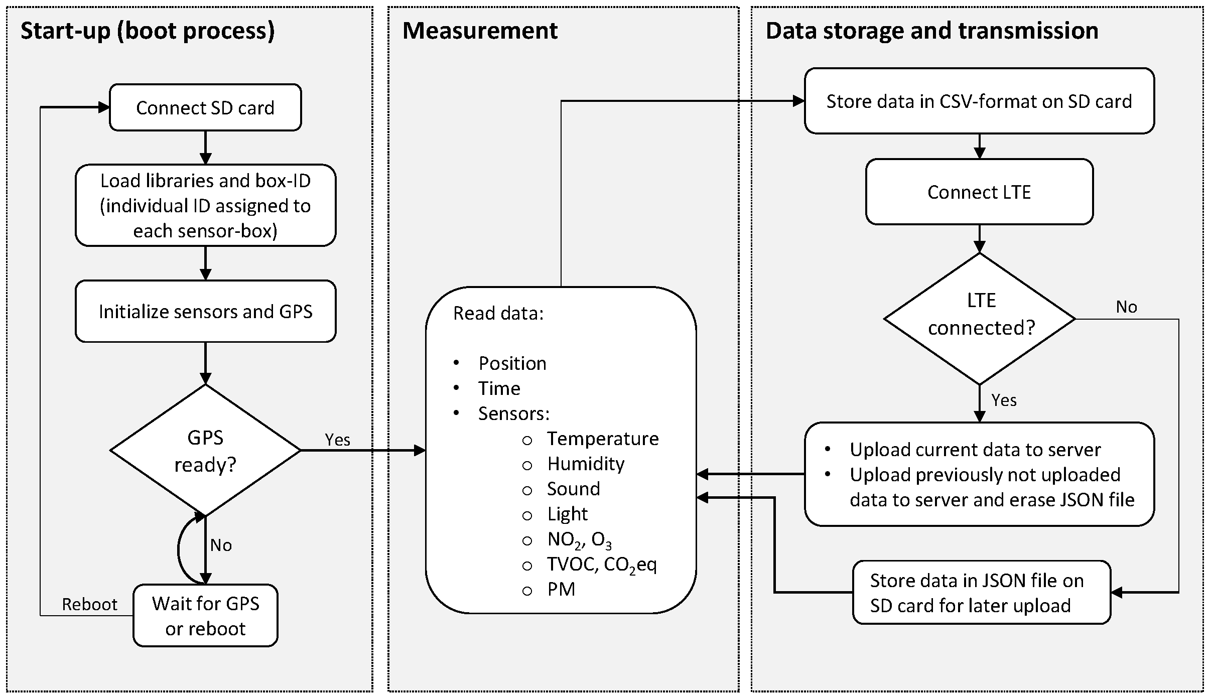
Figure 2.
Software flow chart: sensor-box data acquisition and transmission cycles.
Figure 2.
Software flow chart: sensor-box data acquisition and transmission cycles.
Figure 3.
Validation campaign: sensor-boxes with IDs 1, 2 and 7 placed at the in-luft reference station in Stans.
Figure 3.
Validation campaign: sensor-boxes with IDs 1, 2 and 7 placed at the in-luft reference station in Stans.
Figure 4.
Sensor-box mounted on a utility vehicle from the municipality of Cham.
Figure 4.
Sensor-box mounted on a utility vehicle from the municipality of Cham.
Figure 5.
Validation with reference station: evaluation of filtering methods using PM concentration measurements recorded with stationary sensor-box 2 between 17 November 2021 and 31 December 2021 in Stans, Nidwalden. Displayed is the Pearson correlation coefficient of in-luft and measurement data with different thresholds for the data selection.
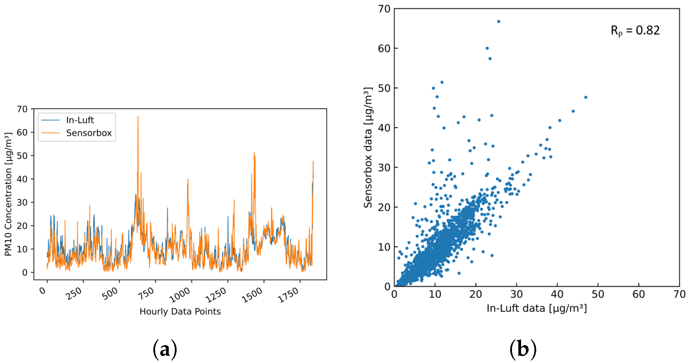
Figure 6.
PM hourly mean data recorded with sensor-box 7 located in Stans in the period from 15 October 2021 to 31 December 2021, compared to hourly mean data recorded at the in-luft station located in Stans. Fixed-percentile (Filter 2, 99.0%) applied to sensor-box data. , , (a) time series; (b) scatter plot.
Figure 7.
Distribution of hourly mean values of PM concentration recorded in Stans, Nidwalden. (a) Sensor-box 1 recorded between 15 October 2021 and 23 December 2021; (b) Sensor-box 2 recorded between 17 November 2021 and 31 December 2021; (c) Sensor-box 7 recorded between 15 October 2021 and 31 December 2021.
Figure 8.
Hourly mean values recorded with sensor-box 1 between 15 October 2021 and 23 December 2021 in Stans, Nidwalden. (a) PM concentration vs. temperature; (b) Distribution of three different PM concentration ranges.
Figure 8.
Hourly mean values recorded with sensor-box 1 between 15 October 2021 and 23 December 2021 in Stans, Nidwalden. (a) PM concentration vs. temperature; (b) Distribution of three different PM concentration ranges.
Figure 9.
Hourly mean values recorded with sensor-box 1 between 4 December 2021 and 24 December 2021 in Stans, Nidwalden compared to in-luft data measured in the same time-interval. (a) PM concentration vs. humidity; (b) PM and humidity time-series data.
Figure 9.
Hourly mean values recorded with sensor-box 1 between 4 December 2021 and 24 December 2021 in Stans, Nidwalden compared to in-luft data measured in the same time-interval. (a) PM concentration vs. humidity; (b) PM and humidity time-series data.
Figure 10.
PM hourly mean data recorded with mobile pilot sensor-boxes in the period from 1 July 2021 to 30 July 2021.
Figure 10.
PM hourly mean data recorded with mobile pilot sensor-boxes in the period from 1 July 2021 to 30 July 2021.
Figure 11.
PM hourly mean data recorded with mobile pilot sensor-boxes in the period from 1 December 2021 to 31 December 2021.
Figure 11.
PM hourly mean data recorded with mobile pilot sensor-boxes in the period from 1 December 2021 to 31 December 2021.
Figure 12.
Pearson correlation and Spearman correlation for mean hourly PM data between sensor-box and in-luft stations compared among different pilot sites. Evaluation of data collected between May and December 2021. Fixed percentile filtering method (99.0%) is applied to the raw sensor-box data.
Figure 12.
Pearson correlation and Spearman correlation for mean hourly PM data between sensor-box and in-luft stations compared among different pilot sites. Evaluation of data collected between May and December 2021. Fixed percentile filtering method (99.0%) is applied to the raw sensor-box data.
Figure 13.
PM hourly mean data recorded with mobile pilot sensor-box 6 located in Luzern in the period from 7 July 2021 to 2 September 2021, compared to hourly mean data recorded at the in-luft station located in Luzern. Data gaps are removed from the graph. Number of mean hourly values: 252; Resulting correlations: , .
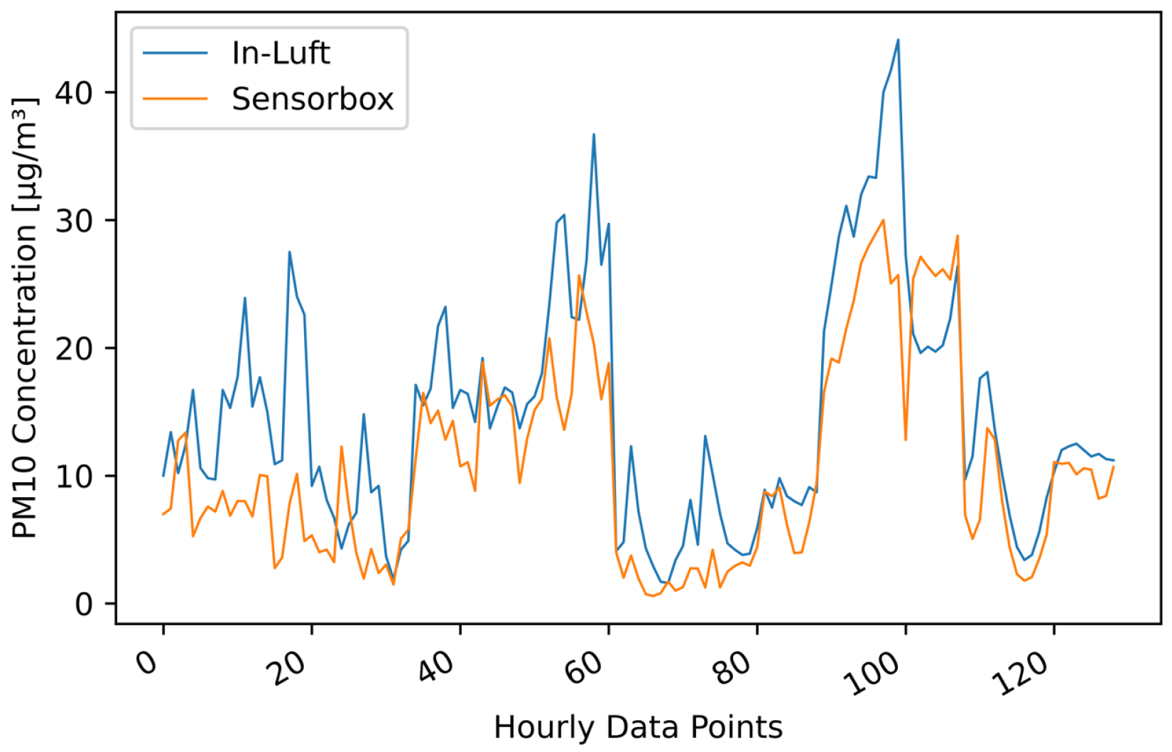
Figure 14.
PM hourly mean data recorded with mobile pilot sensor-box 6 located in Luzern in the period from 7 July 2021 to 2 September 2021, compared to hourly mean data recorded at the in-luft station located in Luzern. Number of mean hourly values: 252; Resulting correlations: , .
Figure 14.
PM hourly mean data recorded with mobile pilot sensor-box 6 located in Luzern in the period from 7 July 2021 to 2 September 2021, compared to hourly mean data recorded at the in-luft station located in Luzern. Number of mean hourly values: 252; Resulting correlations: , .
Figure 15.
PM hourly mean data recorded with mobile pilot sensor-box 6 located in Ebikon in the period from 15 October 2021 to 15 November 2021, compared to hourly mean data recorded at the in-luft station located in Ebikon, Sedel. Data gaps are removed from graph. Number of mean hourly values: 768; Resulting correlations: , .
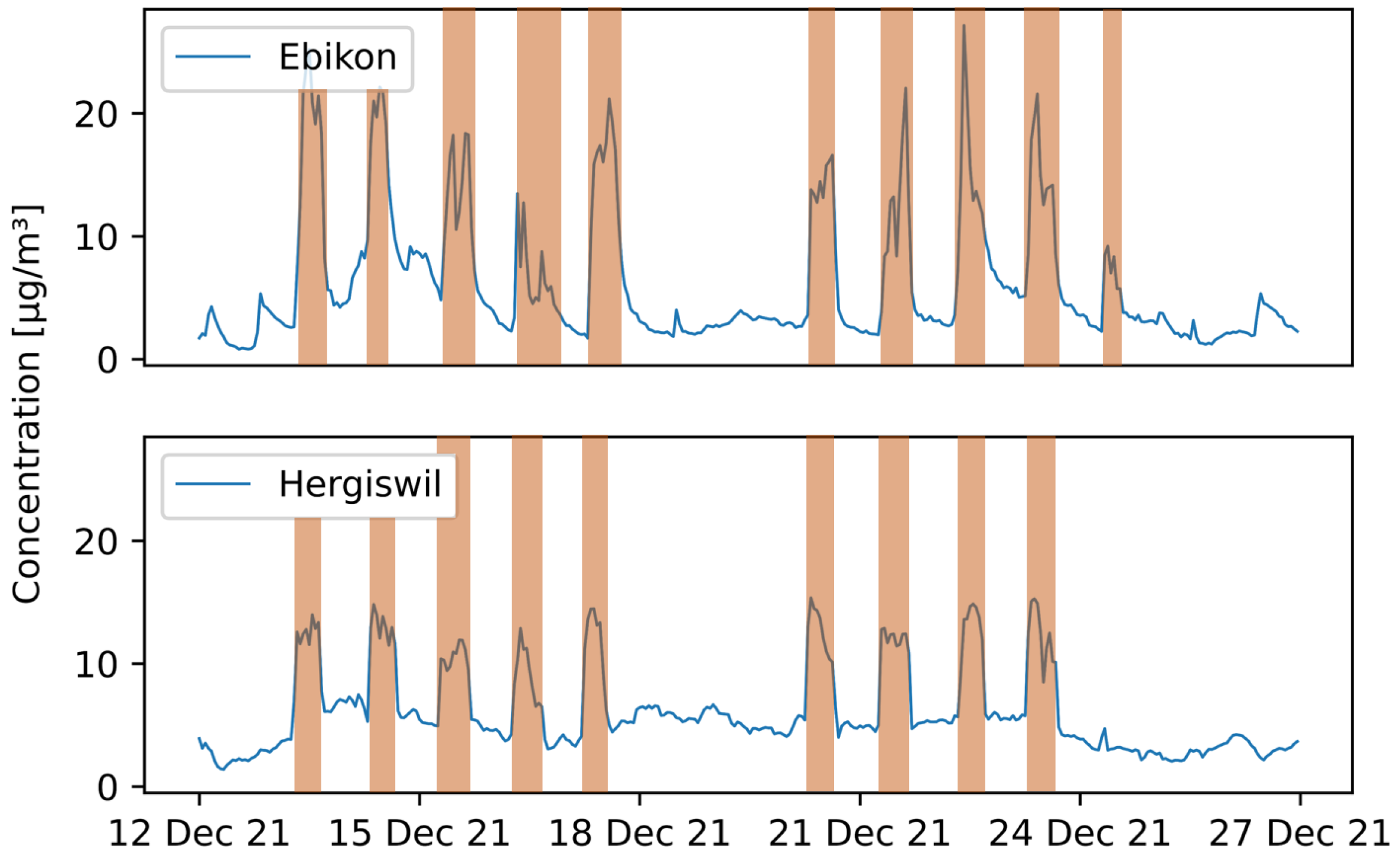
Figure 16.
PM hourly mean data recorded with mobile pilot sensor-boxes located in Ebikon and Hergiswil in the period from 12 December 2021 to 27 December 2021. Periods where the vehicle is in operation are marked in red.
Figure 16.
PM hourly mean data recorded with mobile pilot sensor-boxes located in Ebikon and Hergiswil in the period from 12 December 2021 to 27 December 2021. Periods where the vehicle is in operation are marked in red.
Figure 17.
PM hourly mean data recorded with mobile pilot sensor-box 6 located in Ebikon in the period from 15 October 2021 to 15 November 2021 compared to hourly mean data recorded at the in-luft station located in Ebikon, Sedel. Data gaps are removed from graph. Data recorded within a radius of 150 m around the maintenance depot Ebikon are removed. Number of mean hourly values: N = 129; Resulting correlations: , .
Figure 18.
PM hourly mean data recorded with mobile pilot sensor-box 6 located in Ebikon in the period from 15 October 2021 to 15 November 2021 compared to hourly mean data recorded at the in-luft station located in Ebikon, Sedel. Data recorded within a radius of 150 m around the maintenance depot Ebikon are removed. Number of mean hourly values: N = 129; Resulting correlations: , .
Figure 19.
Geographical location of pilot in Cham and in-luft reference stations Zug and Rigi. (Map source: Federal Office of Topography).
Figure 19.
Geographical location of pilot in Cham and in-luft reference stations Zug and Rigi. (Map source: Federal Office of Topography).
Figure 20.
Hourly mean PM data recorded at in-luft stations Zug and Rigi. (a) , ; (b) , .
Figure 20.
Hourly mean PM data recorded at in-luft stations Zug and Rigi. (a) , ; (b) , .
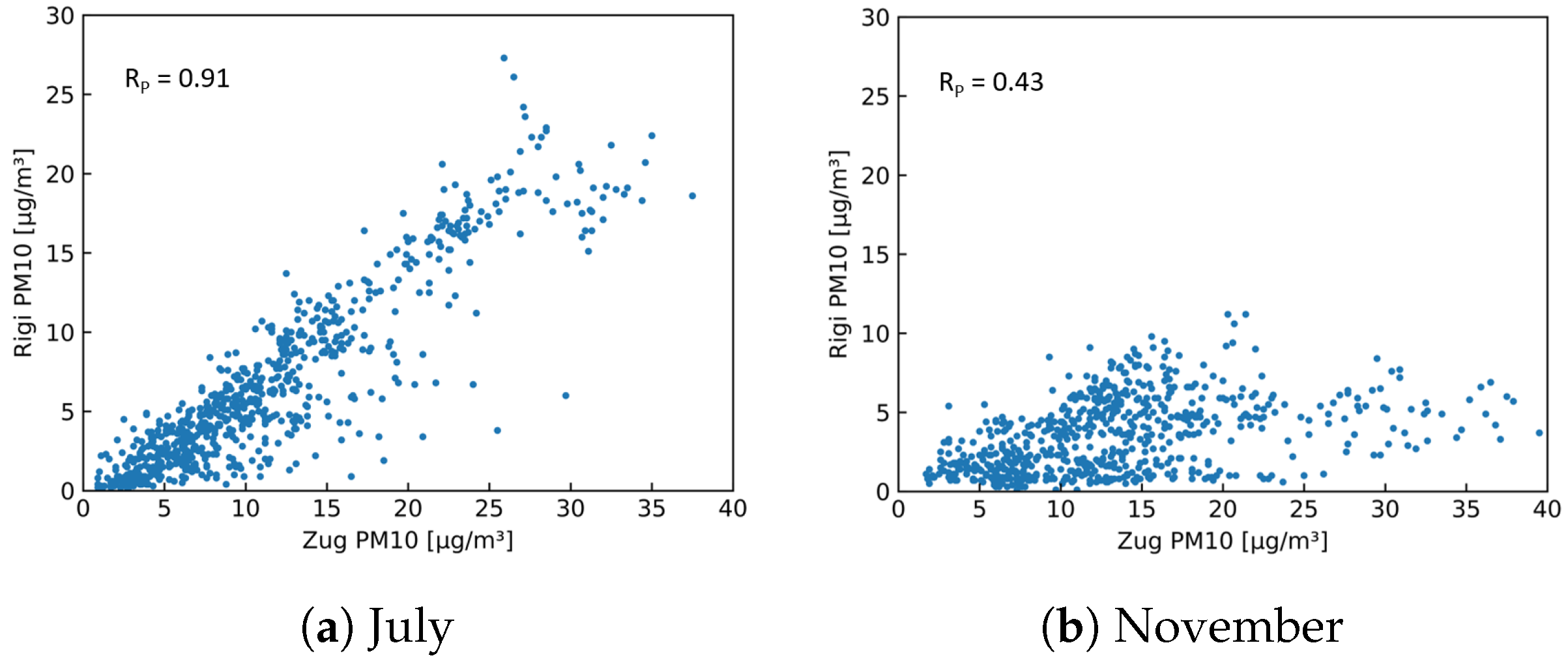
Figure 21.
Hourly mean PM data measured at in-luft stations Zug and Rigi. (a) , ; (b) , .
Figure 21.
Hourly mean PM data measured at in-luft stations Zug and Rigi. (a) , ; (b) , .
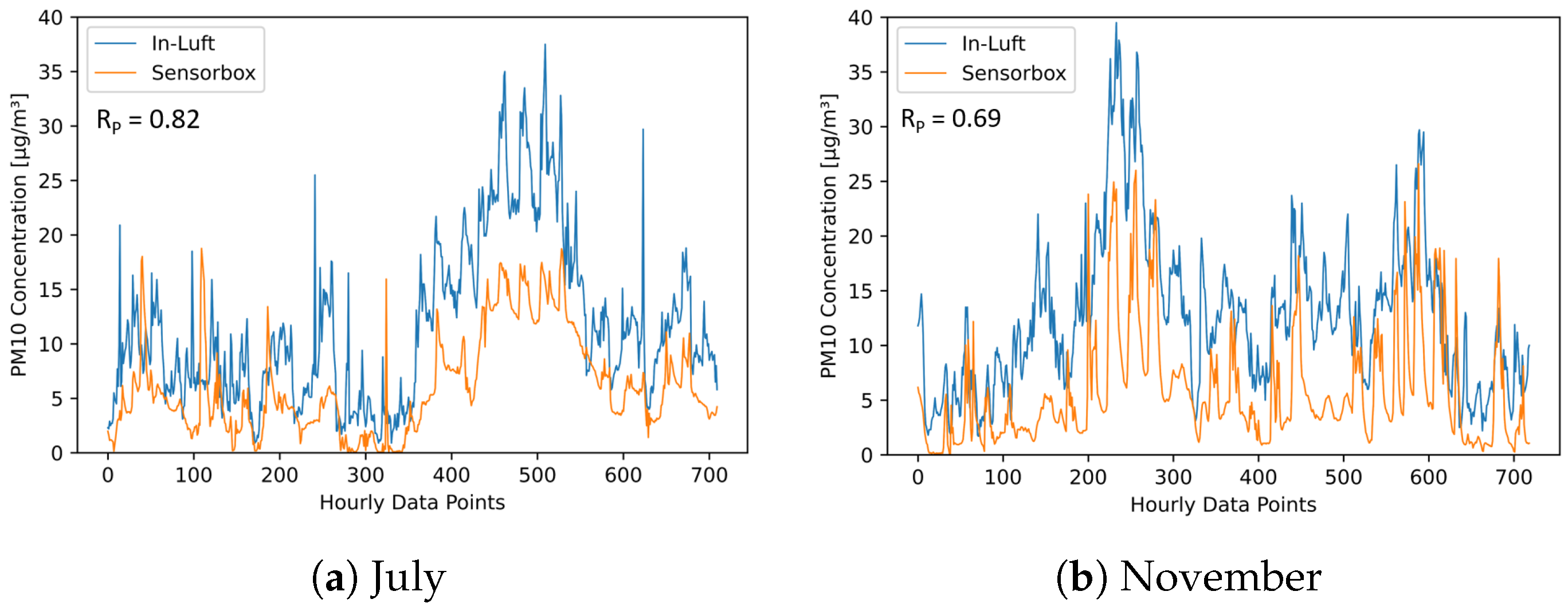
Figure 22.
PM hourly mean data recorded with mobile pilot sensor-box 8 located in Cham compared to hourly mean data recorded at the in-luft station located in Zug, Postplatz. Data gaps are removed from the graph. (a) , , ; (b) , , .
Figure 22.
PM hourly mean data recorded with mobile pilot sensor-box 8 located in Cham compared to hourly mean data recorded at the in-luft station located in Zug, Postplatz. Data gaps are removed from the graph. (a) , , ; (b) , , .
Figure 23.
PM hourly mean data recorded with mobile pilot sensor-box 8 located in Cham compared to hourly mean data recorded at the in-luft station located in Zug, Postplatz. (a) , , ; (b) , , .
Figure 23.
PM hourly mean data recorded with mobile pilot sensor-box 8 located in Cham compared to hourly mean data recorded at the in-luft station located in Zug, Postplatz. (a) , , ; (b) , , .
Figure 24.
PM hourly mean data recorded with mobile pilot sensor-box 8 located in Cham compared to hourly mean data recorded at the in-luft station located in Rigi, Seebodenalp. Data gaps are removed from the graph. (a) , , ; (b) , , .
Figure 24.
PM hourly mean data recorded with mobile pilot sensor-box 8 located in Cham compared to hourly mean data recorded at the in-luft station located in Rigi, Seebodenalp. Data gaps are removed from the graph. (a) , , ; (b) , , .
Figure 25.
PM hourly mean data recorded with mobile pilot sensor-box 8 located in Cham compared to hourly mean data recorded at the in-luft station located in Rigi, Seebodenalp. (a) , , ; (b) , , .
Figure 25.
PM hourly mean data recorded with mobile pilot sensor-box 8 located in Cham compared to hourly mean data recorded at the in-luft station located in Rigi, Seebodenalp. (a) , , ; (b) , , .
Table 1.
Overview of experiments and field tests comparing particulate matter measurements from low-cost sensors to reference instruments.
Table 1.
Overview of experiments and field tests comparing particulate matter measurements from low-cost sensors to reference instruments.
| Location | Experiment Setup and Main Conclusions |
|---|
| | Sensor type; low-cost sensor make; position relative to reference station; environment; results |
| Aveiro, Portugal [16] | Optical; Shinyei PPD42, Shinyei PPD20V, others; side-by-side; outdoors |
| PM10: (0.13–0.36); PM2.5: (0.07–0.27) |
| Oslo, Norway [17] | Optical; AQMesh units; side-by-side; outdoors (dense traffic vs. calm traffic) |
| PM10: (dense traffic), (calm traffic); PM2.5: (dense traffic), (calm traffic); Average match score for PM10 0.91, PM2.5 0.48 |
| Ispra and Brindisi, Italy [22] | Optical; Shinyei PPD20V; side-by-side; outdoors. Period December 2013–March 2014, 1 sample per minute, two locations one rural setting and one industrial site |
| Accuracy of the calibrated optical particle sensor has been calculated as mean error and max error compared to the PM referenced analyzer. They are estimated at 9.0 g/m3 and 41.7 g/m3 |
| Bari, Italy [15] | Optical; Shinyei PPD20V; various locations indoors and outdoors; 11 nodes (10 stationary and 1 mobile mounted on public bus); results are compared to closest air quality monitoring station. |
| MAE 1: 5.6 g/m3, Accuracy 2 in node 1, 2, and 3 is 24.8%, 21.6%, and 20.5%) |
| Helsinki, Finland | Ref. [23]: various types; make not specified; outdoors in 3 different environments (industry with congested traffic; residential with low traffic; mixed residential and university); 100 mobile sensors; 12 fixed sensors; additional sensors side-by-side with reference stations; absolute error after calibration with data in the vicinity of reference stations: PM10 (2.88–17.84 g/m3); PM2.5 (1.38–9.09 g/m3) |
| Ref. [20]: Optical; Panasonic; personal exposure, indoor and outdoor; comparison to reference station 7 km away: R = 0.5 |
| Seoul, South Korea | Ref. [18]: Optical; PMS7003 (Plantower Inc.); outdoors; side-by-side; after calibration (combined linear and non-linear): PM2.5 RMSE = 4.70 g/m3, = 0.89 |
| Ref. [19]: Optical; Sensirion SPS30; side-by-side; PM2.5 after calibration (neural network): (0.59–0.93) |
| Badajoz, Spain [21] | Optical; Alphasense OPC-N3; side-by-side, portable sensor-box validation with a mobile reference measurement station, PM, PM at 3 s resolution, averaged over 10 min and 1 h, |
| PM10: (0.48–0.78); PM2.5: (0.22–0.64) |
Table 2.
Specifications of the Cubic PM3015SN particulate matter sensor [
24]
1.
Table 2.
Specifications of the Cubic PM3015SN particulate matter sensor [
24]
1.
| Specifications | Value |
|---|
| Operating principle | Laser scattering |
| Measured particle size range | 0.3–10 m |
| Measurement range | 0–5000 g/m |
| Resolution | 1 g/m |
| Working condition | to C, 0–95% RH |
| Measurement accuracy PM1.0 and PM2.5 | 0–100 g/m, ±5 g/m |
| | 101–1000 g/m, ±15% of reading |
| | Condition: 25 ± 2 C, 50 ± 10% RH |
| Measurement accuracy PM10 | 0–100 g/m ± 30 g/m |
| | 101–1000 g/m ± 30% of reading |
| | Condition: 25 ± 2 C, 50 ± 10% RH |
| Response time | 1 s |
| Time to first reading | ≤8 s |
Table 3.
Technical specifications of the reference PM measurement station, Fidas200 [
3,
27].
Table 3.
Technical specifications of the reference PM measurement station, Fidas200 [
3,
27].
| Specifications | Value |
|---|
| Operating principle | Laser scattering |
| Particle range | 0.18–18 m |
| Resolution | 0.1 m/m |
| Working condition | 5 to C |
| Measurement accuracy PM2.5 | 9.7% |
| Measurement accuracy PM10 | 7.5 % |
| Response time | <2 s |
Table 4.
Pilot overview of the field test measurement campaign.
Table 4.
Pilot overview of the field test measurement campaign.
| Community | Start | End | Duration (Months) |
|---|
| Hergiswil | April 2021 | April 2022 | 12 |
| Rheinfelden (AEW) | May 2021 | July 2021 | 3 |
| Stansstad | May 2021 | November 2021 | 6 |
| Lostorf | May 2021 | April 2022 | 11 |
| Stans | May 2021 | November 2021 | 6 |
| Horw | May 2021 | April 2022 | 11 |
| Lungern | June 2021 | April 2022 | 10 |
| Kriens | June 2021 | April 2022 | 10 |
| Olten | June 2021 | April 2022 | 10 |
| Malters | June 2021 | March 2022 | 9 |
| Cham | June 2021 | April 2022 | 10 |
| Emmenbruecke | June 2021 | April 2022 | 10 |
| Luzern | July 2021 | April 2022 | 9 |
| Ebikon | September 2021 | April 2022 | 7 |
Table 5.
Stationary sensor-boxes in Stans, Nidwalden.
Table 5.
Stationary sensor-boxes in Stans, Nidwalden.
| Sensor-Box ID | Start–End | Duration | Data Points |
|---|
| 1 | 15 October–23 December 2021 | 2 months | 107,338 |
| 2 | 17 November–31 December 2021 | 1.5 months | 71,149 |
| 7 | 15 October–31 December 2021 | 2.5 months | 134,768 |
Table 6.
Results of statistical analysis of stationary senor-box measurements in Stans, Nidwalden. Measurements recorded between 15 October 2021 and 31 December 2021. Fixed percentile filtering method (99.0%) is applied to the raw data. No further calibration applied.
Table 6.
Results of statistical analysis of stationary senor-box measurements in Stans, Nidwalden. Measurements recorded between 15 October 2021 and 31 December 2021. Fixed percentile filtering method (99.0%) is applied to the raw data. No further calibration applied.
| Sensor-Box ID | MAE (g/m) | RMSE (g/m) | Slope | Intercept (g/m) | | | Bias (%) |
|---|
| 1 | 5.44 | 10.38 | 1.60 | −2.14 | 0.74 | 0.88 | 30.30 |
| 2 | 3.70 | 8.23 | 1.28 | 0.06 | 0.72 | 0.87 | 27.40 |
| 7 | 2.52 | 4.38 | 1.01 | −0.79 | 0.82 | 0.90 | −10.73 |
Table 7.
Overview of usable data sets collected between May and December 2021 in Central Switzerland.
Table 7.
Overview of usable data sets collected between May and December 2021 in Central Switzerland.
| Data Set | Pilot | Sensor-Box | In-Luft Station | Distance | Hourly Data Points |
|---|
| (A) | Cham | 8 | Zug | 5 km | 4401 |
| (B) | Ebikon | 14 | Ebikon | 3 km | 240 |
| (C) | 6 | 1878 |
| (D) | Emmenbruecke | 13 | Ebikon | 1 km | 166 |
| (E) | 15 | 1127 |
| (F) | Hergiswil | 5 | Stans | 5 km | 2125 |
| (G) | 4 | 477 |
| (H) | 15 | 1210 |
| (I) | Horw | 7 | Luzern | 4 km | 118 |
| (J) | 3 | 1226 |
| (K) | 14 | 155 |
| (L) | 4 | 337 |
| (M) | Kriens | 9 | Luzern | 3 km | 4073 |
| (N) | Luzern | 6 | Luzern | 0 km | 252 |
| (O) | 12 | 401 |
| (P) | Malters | 2 | Luzern | 9 km | 75 |
| (Q) | 10 | 3305 |
| (R) | Stans | 15 | Stans | 2 km | 1223 |
| (S) | Stansstad | 2 | Stans | 3 km | 784 |
| (T) | 11 | 837 |
| (U) | 13 | 2214 |
Table 8.
Results of statistical analysis of pilot data against in-luft data for data collected between May and December 2021. Fixed percentile filtering method (99.0%) is applied to the raw data. No further calibration applied.
Table 8.
Results of statistical analysis of pilot data against in-luft data for data collected between May and December 2021. Fixed percentile filtering method (99.0%) is applied to the raw data. No further calibration applied.
| Data Set | MAE (g/m) | RMSE (g/m) | Slope | Intercept (g/m) | | | Bias (%) |
|---|
| (A) | 6.71 | 8.39 | 0.44 | 0.59 | 0.69 | 0.75 | −49.71 |
| (B) | 6.72 | 7.58 | 0.53 | −0.51 | 0.80 | 0.81 | −47.53 |
| (C) | 8.36 | 10.32 | 0.36 | 1.09 | 0.48 | 0.54 | −44.30 |
| (D) | 3.47 | 4.28 | 0.29 | 2.85 | 0.37 | 0.48 | −26.34 |
| (E) | 6.95 | 9.45 | 0.28 | 2.78 | 0.76 | 0.79 | −41.03 |
| (F) | 4.89 | 6.19 | 0.47 | −0.07 | 0.82 | 0.86 | −57.16 |
| (G) | 7.26 | 8.68 | 0.44 | −1.25 | 0.60 | 0.65 | −71.36 |
| (H) | 5.86 | 7.59 | 0.34 | 1.12 | 0.63 | 0.74 | −50.16 |
| (I) | 3.36 | 3.88 | 0.36 | −0.07 | 0.60 | 0.67 | −66.07 |
| (J) | 6.89 | 9.06 | 0.32 | 1.13 | 0.88 | 0.91 | −54.90 |
| (K) | 9.18 | 10.17 | 0.59 | −2.69 | 0.77 | 0.73 | −61.31 |
| (L) | 7.27 | 8.93 | 0.25 | 1.13 | 0.43 | 0.69 | −62.07 |
| (M) | 10.02 | 12.58 | 0.23 | 1.79 | 0.69 | 0.76 | −58.40 |
| (N) | 6.47 | 7.79 | 0.46 | 0.02 | 0.83 | 0.80 | −52.12 |
| (O) | 8.14 | 10.43 | 0.53 | 0.60 | 0.70 | 0.79 | −45.62 |
| (P) | 2.49 | 3.18 | 0.09 | 5.60 | 0.21 | 0.21 | −1.20 |
| (Q) | 12.52 | 15.00 | 0.09 | 1.48 | 0.44 | 0.64 | −76.81 |
| (R) | 4.93 | 6.05 | 0.36 | 1.22 | 0.75 | 0.78 | −42.14 |
| (S) | 2.67 | 4.27 | 0.45 | 3.88 | 0.39 | 0.58 | 47.14 |
| (T) | 7.98 | 11.03 | 0.04 | 1.33 | 0.58 | 0.54 | −72.49 |
| (U) | 6.08 | 9.03 | 0.52 | 4.52 | 0.34 | 0.62 | 10.93 |
Table 9.
Analysis of statistical metrics across all 21 pilot data sets.
Table 9.
Analysis of statistical metrics across all 21 pilot data sets.
| | Mean | Min. | Max. | SD | Variance | CV (%) |
|---|
| 0.61 | 0.21 | 0.88 | 0.18 | 0.03 | 30.09 |
| 0.68 | 0.21 | 0.91 | 0.15 | 0.02 | 22.23 |
| Slope | 0.35 | 0.04 | 0.59 | 0.15 | 0.02 | 42.41 |
| Intercept | 1.26 | −2.69 | 5.60 | 1.86 | 3.46 | 147.14 |
| Bias | −43.94 | −76.82 | 47.14 | 29.18 | 851.48 | −66.42 |
| MAE | 6.58 | 2.49 | 12.52 | 2.40 | 5.77 | 36.49 |
| RMSE | 8.28 | 3.18 | 15.00 | 2.88 | 8.32 | 34.84 |
Table 10.
Location profile of in-luft reference stations [
47].
Table 10.
Location profile of in-luft reference stations [
47].
| Specification | Zug | Rigi |
|---|
| Geography | midlands | pre-alpine |
| Location | city center; close to lake | rural area; in open field close to forest |
| Altitude | 420 m.a.s.l. | 1031 m.a.s.l. |
| Settlement size | 26,000 | n/a |
| Distance to road | 24 m | n/a |


 ,
, 


