

Interval Type-II Fuzzy Fault-Tolerant Control for Constrained Uncertain 2-DOF Robotic Multi-Agent Systems with Active Fault Detection


Abstract
1. Introduction
2. Preliminaries
3. Problem Description
4. Results
4.1. Active Fault Detection and Fault-Tolerant Control
| Algorithm 1 Active fault-detection algorithm () |
|
4.2. Main Controller Design
4.2.1. Main Controller Design of Leader
4.2.2. Main Controller Design of Follower
4.3. Redundant Controller Design
| Algorithm 2 Active fault-tolerant control algorithm () |
|
4.4. Stability Analysis of the System
5. Simulation
5.1. Validation Simulations of the Proposed Controller for Single-Agent Systems
5.2. Validation Simulations of the Proposed Controller for Multi-Agent Systems
5.3. Comparative Simulations between the Proposed Method and the Passive Fault-Tolerant Method
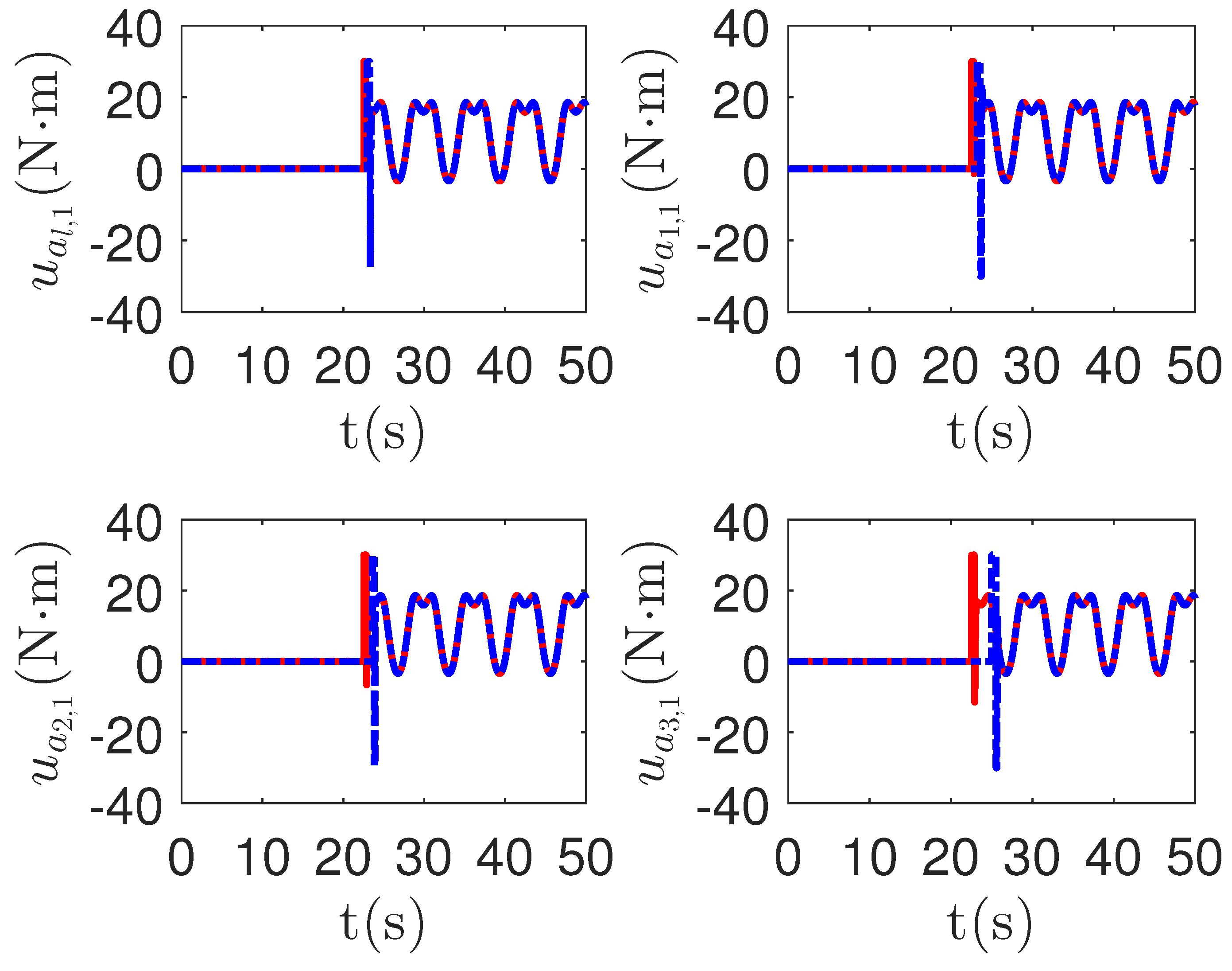
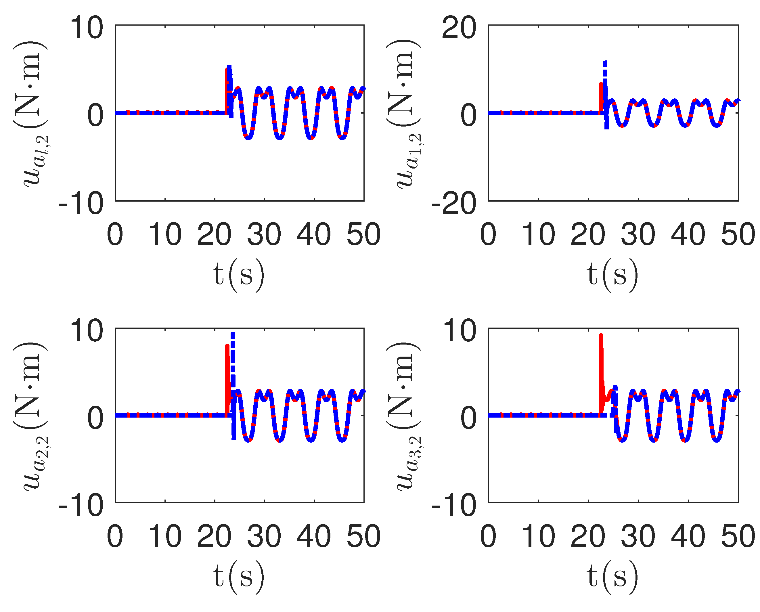
5.4. The Comparative Simulations between the Proposed Method and Active Fault-Tolerant Method
6. Conclusions
Author Contributions
Funding
Institutional Review Board Statement
Informed Consent Statement
Data Availability Statement
Conflicts of Interest
Appendix A
Appendix B
Appendix C
References
- Wang, X.; Park, J.H.; Yang, H. An improved protocol to consensus of delayed MASs with UNMS and aperiodic DoS cyber-attacks. IEEE Trans. Netw. Sci. Eng. 2021, 8, 2506–2516. [Google Scholar] [CrossRef]
- Jiang, Y.; Niu, B.; Wang, X.; Zhao, X.; Wang, H.; Yan, B. Distributed finite-time consensus tracking control for nonlinear multi-agent systems with FDI attacks and application to single-link robots. IEEE Trans. Circuits Syst. II Express Briefs 2022, 70, 1505–1509. [Google Scholar] [CrossRef]
- Zhang, K.; Zhao, T.; Dian, S. Dynamic output feedback control for nonlinear networked control systems with a two-terminal event-triggered mechanism. Nonlinear Dyn. 2020, 100, 2537–2555. [Google Scholar] [CrossRef]
- Zhao, T.; Li, H.; Dian, S. Multi-robot path planning based on improved artificial potential field and fuzzy inference system. J. Intell. Fuzzy Syst. 2020, 39, 7621–7637. [Google Scholar] [CrossRef]
- Chen, W.D.; Li, Y.X.; Liu, L.; Zhao, X.D.; Niu, B.; Han, L.M. Nussbaum-Based Adaptive Fault-Tolerant Control for Nonlinear CPSs With Deception Attacks: A New Coordinate Transformation Technology. IEEE Trans. Cybern. 2022. [Google Scholar] [CrossRef] [PubMed]
- Wang, H.; Ma, J.; Zhao, X.; Niu, B.; Chen, M.; Wang, W. Adaptive Fuzzy Fixed-Time Control for High-Order Nonlinear Systems With Sensor and Actuator Faults. IEEE Trans. Fuzzy Syst. 2023. [Google Scholar] [CrossRef]
- Amin, A.A.; Hasan, K.M. A review of fault tolerant control systems: Advancements and applications. Measurement 2019, 143, 58–68. [Google Scholar] [CrossRef]
- Wang, X.; Niu, B.; Song, X.; Zhao, P.; Wang, Z. Neural networks-based adaptive practical preassigned finite-time fault tolerant control for nonlinear time-varying delay systems with full state constraints. Int. J. Robust Nonlinear Control 2021, 31, 1497–1513. [Google Scholar] [CrossRef]
- Li, Q.; Wu, Q.; Tu, H.; Zhang, J.; Zou, X.; Huang, S. Ground Risk Assessment for Unmanned Aircraft Focusing on Multiple Risk Sources in Urban Environments. Processes 2023, 11, 542. [Google Scholar] [CrossRef]
- Zhang, Y.; Jiang, J. Bibliographical review on reconfigurable fault-tolerant control systems. Annu. Rev. Control 2008, 32, 229–252. [Google Scholar] [CrossRef]
- Zhang, Y.; Jiang, J. Active fault-tolerant control system against partial actuator failures. IEE Proc. Control Theory Appl. 2002, 149, 95–104. [Google Scholar] [CrossRef]
- Maki, M.; Jiang, J.; Hagino, K. A stability guaranteed active fault-tolerant control system against actuator failures. Int. J. Robust Nonlinear Control IFAC Affil. J. 2004, 14, 1061–1077. [Google Scholar] [CrossRef]
- Merheb, A.R.; Noura, H.; Bateman, F. Active fault tolerant control of quadrotor uav using sliding mode control. In Proceedings of the 2014 International Conference on Unmanned Aircraft Systems (ICUAS), Orlando, FL, USA, 27–30 May 2014; pp. 156–166. [Google Scholar]
- Hosseinnajad, A.; Loueipour, M. Design of finite-time active fault tolerant control system with real-time fault estimation for a remotely operated vehicle. Ocean Eng. 2021, 241, 110063. [Google Scholar] [CrossRef]
- Li, J.; Xiang, X.; Dong, D.; Yang, S. Prescribed time observer based trajectory tracking control of autonomous underwater vehicle with tracking error constraints. Ocean Eng. 2023, 274, 114018. [Google Scholar] [CrossRef]
- Zhang, J.; Niu, B.; Wang, D.; Wang, H.; Zhao, P.; Zong, G. Time-/event-triggered adaptive neural asymptotic tracking control for nonlinear systems with full-state constraints and application to a single-link robot. IEEE Trans. Neural Netw. Learn. Syst. 2021, 33, 6690–6700. [Google Scholar] [CrossRef]
- Tang, H.; Gao, S.; Wang, L.; Li, X.; Li, B.; Pang, S. A novel intelligent fault diagnosis method for rolling bearings based on Wasserstein generative adversarial network and Convolutional Neural Network under Unbalanced Dataset. Sensors 2021, 21, 6754. [Google Scholar] [CrossRef]
- Xiao, L.; Bajric, R.; Zhao, J.; Tang, J.; Zhang, X. An adaptive vibrational resonance method based on cascaded varying stable-state nonlinear systems and its application in rotating machine fault detection. Nonlinear Dyn. 2021, 103, 715–739. [Google Scholar] [CrossRef]
- Bzioui, S.; Channa, R. Estimation and fault diagnosis for non-linear system with time-varying faults and measurement noises: Application on two CSTRs in series. Can. J. Chem. Eng. 2023, 101, 1919–1930. [Google Scholar] [CrossRef]
- Gao, Y.; Xiao, F.; Liu, J.; Wang, R. Distributed soft fault detection for interval type-2 fuzzy-model-based stochastic systems with wireless sensor networks. IEEE Trans. Ind. Inform. 2018, 15, 334–347. [Google Scholar] [CrossRef]
- Hebda-Sobkowicz, J.; Zimroz, R.; Pitera, M.; Wyłomańska, A. Informative frequency band selection in the presence of non-Gaussian noise—A novel approach based on the conditional variance statistic with application to bearing fault diagnosis. Mech. Syst. Signal Process. 2020, 145, 106971. [Google Scholar] [CrossRef]
- Zhang, G.; Shu, Y.; Zhang, T. Piecewise unsaturated multi-stable stochastic resonance under trichotomous noise and its application in bearing fault diagnosis. Results Phys. 2021, 30, 104907. [Google Scholar] [CrossRef]
- Stojanovic, V.; Prsic, D. Robust identification for fault detection in the presence of non-Gaussian noises: Application to hydraulic servo drives. Nonlinear Dyn. 2020, 100, 2299–2313. [Google Scholar] [CrossRef]
- Zhang, G.; Zhang, Y.; Zhang, T.; Mdsohel, R. Stochastic resonance in an asymmetric bistable system driven by multiplicative and additive Gaussian noise and its application in bearing fault detection. Chin. J. Phys. 2018, 56, 1173–1186. [Google Scholar] [CrossRef]
- Zhao, H.; Yang, X.; Chen, B.; Chen, H.; Deng, W. Bearing fault diagnosis using transfer learning and optimized deep belief network. Meas. Sci. Technol. 2022, 33, 065009. [Google Scholar] [CrossRef]
- Zhao, H.; Zhang, P.; Zhang, R.; Yao, R.; Deng, W. A novel performance trend prediction approach using ENBLS with GWO. Meas. Sci. Technol. 2022, 34, 025018. [Google Scholar] [CrossRef]
- Andjelkovic, I.; Sweetingham, K.; Campbell, S.L. Active fault detection in nonlinear systems using auxiliary signals. In Proceedings of the 2008 American Control Conference, Seattle, WA, USA, 11–13 June 2008; pp. 2142–2147. [Google Scholar]
- Ashari, A.E.; Nikoukhah, R.; Campbell, S.L. Effects of feedback on active fault detection. Automatica 2012, 48, 866–872. [Google Scholar] [CrossRef]
- Punčochář, I.; Širokỳ, J.; Šimandl, M. Constrained active fault detection and control. IEEE Trans. Autom. Control 2014, 60, 253–258. [Google Scholar] [CrossRef]
- Jia, F.; Cao, F.; Lyu, G.; He, X. A novel framework of cooperative design: Bringing active fault diagnosis into fault-tolerant control. IEEE Trans. Cybern. 2022, 53, 3301–3310. [Google Scholar] [CrossRef]
- Jiang, Y.; Niu, B.; Wang, X.; Wang, H.; Chen, W. Dynamic-estimator-based adaptive secure containment control for constrained nonlinear multi-agent systems under denial-of-service attacks. Int. J. Robust Nonlinear Control 2023, 33, 605–622. [Google Scholar] [CrossRef]
- Zhao, T.; Dian, S. State feedback control for interval type-2 fuzzy systems with time-varying delay and unreliable communication links. IEEE Trans. Fuzzy Syst. 2017, 26, 951–966. [Google Scholar] [CrossRef]
- Wang, X.; Park, J.H.; She, K.; Zhong, S.; Shi, L. Stabilization of chaotic systems with T–S fuzzy model and nonuniform sampling: A switched fuzzy control approach. IEEE Trans. Fuzzy Syst. 2018, 27, 1263–1271. [Google Scholar] [CrossRef]
- Qin, P.; Zhao, T.; Dian, S. Interval type-2 fuzzy neural network-based adaptive compensation control for omni-directional mobile robot. Neural Comput. Appl. 2023, 1–15. [Google Scholar] [CrossRef]
- Zhao, J.; Zhao, T.; Liu, N. Fractional-Order Active Disturbance Rejection Control with Fuzzy Self-Tuning for Precision Stabilized Platform. Entropy 2022, 24, 1681. [Google Scholar] [CrossRef] [PubMed]
- Xiu, Z.; Wang, Y.; Cheng, Z. Stability analysis and design of Type-II fuzzy controllers. In Proceedings of the 2008 Chinese Control and Decision Conference, Yantai, China, 2–4 July 2008; pp. 2054–2059. [Google Scholar]
- Mohagheghi, S.; Venayagamoorthy, G.K.; Harley, R.G. An interval Type-II robust fuzzy logic controller for a static compensator in a multimachine power system. In Proceedings of the 2006 IEEE International Joint Conference on Neural Network Proceedings, Vancouver, BC, Canada, 16–21 July 2006; pp. 2241–2248. [Google Scholar]
- Tang, F.; Niu, B.; Wang, H.; Zhang, L.; Zhao, X. Adaptive fuzzy tracking control of switched MIMO nonlinear systems with full state constraints and unknown control directions. IEEE Trans. Circuits Syst. Express Briefs 2022, 69, 2912–2916. [Google Scholar] [CrossRef]
- Dian, S.; Hu, Y.; Zhao, T.; Han, J. Adaptive backstepping control for flexible-joint manipulator using interval type-2 fuzzy neural network approximator. Nonlinear Dyn. 2019, 97, 1567–1580. [Google Scholar] [CrossRef]
- Tong, W.; Zhao, T.; Duan, Q.; Zhang, H.; Mao, Y. Non-singleton interval type-2 fuzzy PID control for high precision electro-optical tracking system. ISA Trans. 2022, 120, 258–270. [Google Scholar] [CrossRef]
- Wang, J.; Hu, L.; Chen, F.; Wen, C. Multiple-step fault estimation for interval type-II TS fuzzy system of hypersonic vehicle with time-varying elevator faults. Int. J. Adv. Robot. Syst. 2017, 14, 1729881417699149. [Google Scholar] [CrossRef]
- Patel, H.; Shah, V. Actuator and system component fault tolerant control using interval type-2 Takagi-Sugeno fuzzy controller for hybrid nonlinear process. Int. J. Hybrid Intell. Syst. 2019, 15, 143–153. [Google Scholar] [CrossRef]
- Yeh, C.C.; Demerdash, N.A. Fault-tolerant soft starter control of induction motors with reduced transient torque pulsations. IEEE Trans. Energy Convers. 2009, 24, 848–859. [Google Scholar]
- Yang, L.; Ozay, N. Fault-tolerant output-feedback path planning with temporal logic constraints. In Proceedings of the 2018 IEEE Conference on Decision and Control (CDC), Miami, FL, USA, 17–19 December 2018; pp. 4032–4039. [Google Scholar]
- Li, Z.; Jamshidian, M.; Mousavi, S.; Karimipour, A.; Tlili, I. Develop a numerical approach of fuzzy logic type-2 to improve the reliability of a hydraulic automated guided vehicles. Int. J. Numer. Methods Heat Fluid Flow 2021, 31, 1396–1409. [Google Scholar] [CrossRef]
- Lin, M.; Huang, C.; Xu, Z.; Chen, R. Evaluating IoT platforms using integrated probabilistic linguistic MCDM method. IEEE Internet Things J. 2020, 7, 11195–11208. [Google Scholar] [CrossRef]
- Huang, C.; Lin, M.; Xu, Z. Pythagorean fuzzy MULTIMOORA method based on distance measure and score function: Its application in multicriteria decision making process. Knowl. Inf. Syst. 2020, 62, 4373–4406. [Google Scholar] [CrossRef]
- Lin, M.; Huang, C.; Xu, Z. TOPSIS method based on correlation coefficient and entropy measure for linguistic Pythagorean fuzzy sets and its application to multiple attribute decision making. Complexity 2019, 2019, 6967390. [Google Scholar] [CrossRef]
- Lin, M.; Wang, H.; Xu, Z. TODIM-based multi-criteria decision-making method with hesitant fuzzy linguistic term sets. Artif. Intell. Rev. 2020, 53, 3647–3671. [Google Scholar] [CrossRef]
- Lin, M.; Li, X.; Chen, R.; Fujita, H.; Lin, J. Picture fuzzy interactional partitioned Heronian mean aggregation operators: An application to MADM process. Artif. Intell. Rev. 2022, 55, 1171–1208. [Google Scholar] [CrossRef]
- Lin, M.; Huang, C.; Chen, R.; Fujita, H.; Wang, X. Directional correlation coefficient measures for Pythagorean fuzzy sets: Their applications to medical diagnosis and cluster analysis. Complex Intell. Syst. 2021, 7, 1025–1043. [Google Scholar] [CrossRef]
- Zhou, Q.; Wang, L.; Wu, C.; Li, H.; Du, H. Adaptive fuzzy control for nonstrict-feedback systems with input saturation and output constraint. IEEE Trans. Syst. Man Cybern. Syst. 2016, 47, 1–12. [Google Scholar] [CrossRef]
- Zhou, X.; Cai, X.; Zhang, H.; Zhang, Z.; Jin, T.; Chen, H.; Deng, W. Multi-strategy competitive-cooperative co-evolutionary algorithm and its application. Inf. Sci. 2023, 635, 328–344. [Google Scholar] [CrossRef]
- Zhao, T.; Chen, C.; Cao, H. Evolutionary self-organizing fuzzy system using fuzzy-classification-based social learning particle swarm optimization. Inf. Sci. 2022, 606, 92–111. [Google Scholar] [CrossRef]
- Li, M.; Zhang, J.; Song, J.; Li, Z.; Lu, S. A Clinical-Oriented Non-Severe Depression Diagnosis Method Based on Cognitive Behavior of Emotional Conflict. IEEE Trans. Comput. Soc. Syst. 2022, 10, 131–141. [Google Scholar] [CrossRef]
- Zhao, T.; Chen, C.; Cao, H.; Dian, S.; Xie, X. Multiobjective Optimization design of interpretable evolutionary fuzzy systems with type self-organizing learning of fuzzy sets. IEEE Trans. Fuzzy Syst. 2022, 31, 1638–1652. [Google Scholar] [CrossRef]
- Huang, C.; Zhou, X.; Ran, X.; Liu, Y.; Deng, W.; Deng, W. Co-evolutionary competitive swarm optimizer with three-phase for large-scale complex optimization problem. Inf. Sci. 2023, 619, 2–18. [Google Scholar] [CrossRef]
- Zhao, T.; Cao, H.; Dian, S. A self-organized method for a hierarchical fuzzy logic system based on a fuzzy autoencoder. IEEE Trans. Fuzzy Syst. 2022, 30, 5104–5115. [Google Scholar] [CrossRef]
- Zhao, T.; Tong, W.; Mao, Y. Hybrid Non-singleton Fuzzy Strong Tracking Kalman Filtering for High Precision Photoelectric Tracking System. IEEE Trans. Ind. Inform. 2023, 19, 2395–2408. [Google Scholar] [CrossRef]
- Rudin, K.; Ducard, G.J.; Siegwart, R.Y. Active fault-tolerant control with imperfect fault detection information: Applications to UAVs. IEEE Trans. Aerosp. Electron. Syst. 2019, 56, 2792–2805. [Google Scholar] [CrossRef]
- Liberzon, D.; Morse, A.S. Basic problems in stability and design of switched systems. IEEE Control Syst. Mag. 1999, 19, 59–70. [Google Scholar]
- Liu, Y.; Yan, W.; Yu, C.; Zhang, T.; Tu, H. Predefined-Time Trajectory Planning for a Dual-Arm Free-Floating Space Robot. In Proceedings of the IECON 2020 The 46th Annual Conference of the IEEE Industrial Electronics Society, Singapore, 18–21 October 2020; pp. 2798–2803. [Google Scholar]
- Yan, W.; Liu, Y.; Lan, Q.; Zhang, T.; Tu, H. Trajectory planning and low-chattering fixed-time nonsingular terminal sliding mode control for a dual-arm free-floating space robot. Robotica 2022, 40, 625–645. [Google Scholar] [CrossRef]
- Yao, J.; Yan, W.; Lan, Q.; Liu, Y.; Zhao, Y. Parameter Optimization of dsRNA Splicing Evolutionary Algorithm Based Fixed-Time Obstacle-Avoidance Trajectory Planning for Space Robot. Appl. Sci. 2021, 11, 8839. [Google Scholar] [CrossRef]
- Liu, Y.; Yan, W.; Zhang, T.; Yu, C.; Tu, H. Trajectory tracking for a dual-arm free-floating space robot with a class of general nonsingular predefined-time terminal sliding mode. IEEE Trans. Syst. Man Cybern. Syst. 2021, 52, 3273–3286. [Google Scholar] [CrossRef]
- Yan, B.; Niu, B.; Zhao, X.; Wang, H.; Chen, W.; Liu, X. Neural-network-based adaptive event-triggered asymptotically consensus tracking control for nonlinear nonstrict-feedback MASs: An improved dynamic surface approach. IEEE Trans. Neural Netw. Learn. Syst. 2022. [Google Scholar] [CrossRef]
- Van, M.; Sun, Y.; Mcllvanna, S.; Nguyen, M.N.; Khyam, M.O.; Ceglarek, D. Adaptive Fuzzy Fault Tolerant Control for Robot Manipulators with Fixed-Time Convergence. IEEE Trans. Fuzzy Syst. 2023. [Google Scholar] [CrossRef]
- Ouyang, H.; Lin, Y. Adaptive fault-tolerant control and performance recovery against actuator failures with deferred actuator replacement. IEEE Trans. Autom. Control 2020, 66, 3810–3817. [Google Scholar] [CrossRef]


 : ;
: ; : .
: ;: .
: .
: ;: . : ;: .
: ;: .
: ;: . : ;: .
: ;: .
: ;: . : The proposed method;
 : The passive fault-tolerant control method [67].
 : The proposed method;: The passive fault-tolerant control method [67].
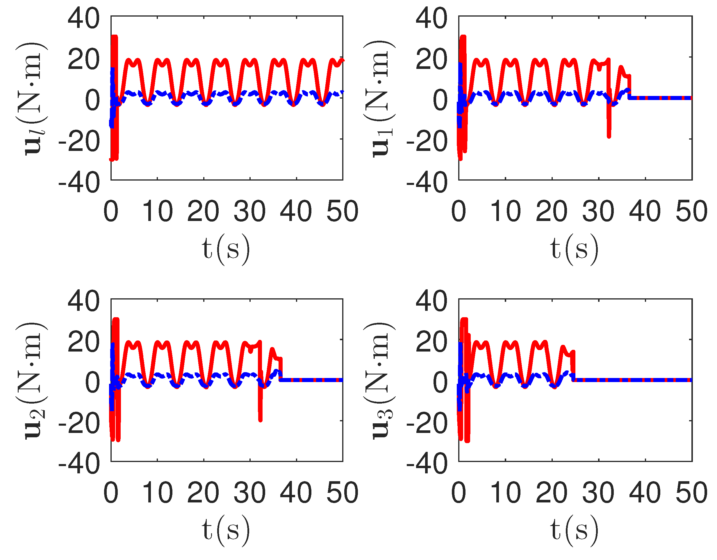
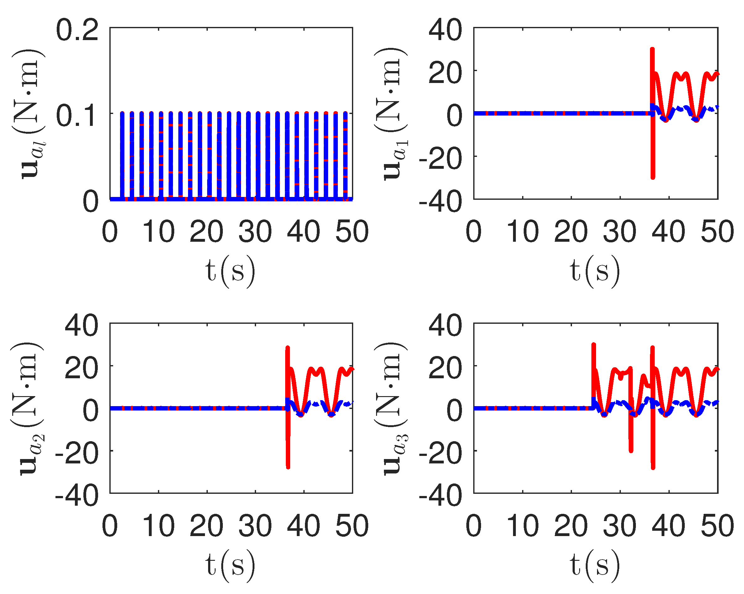
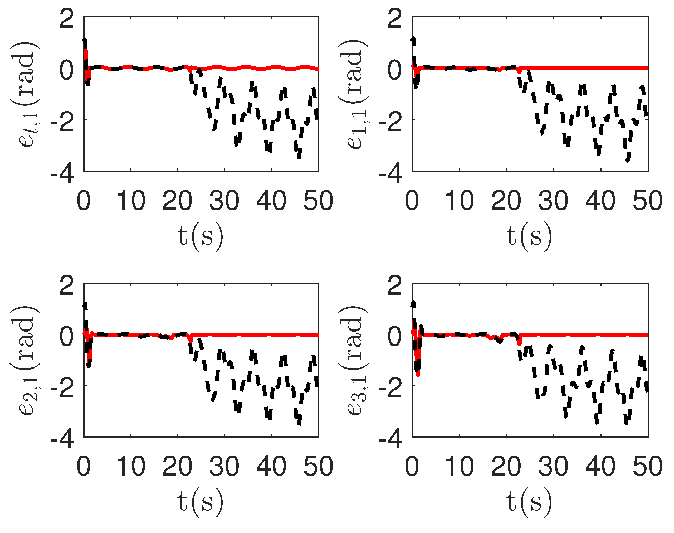
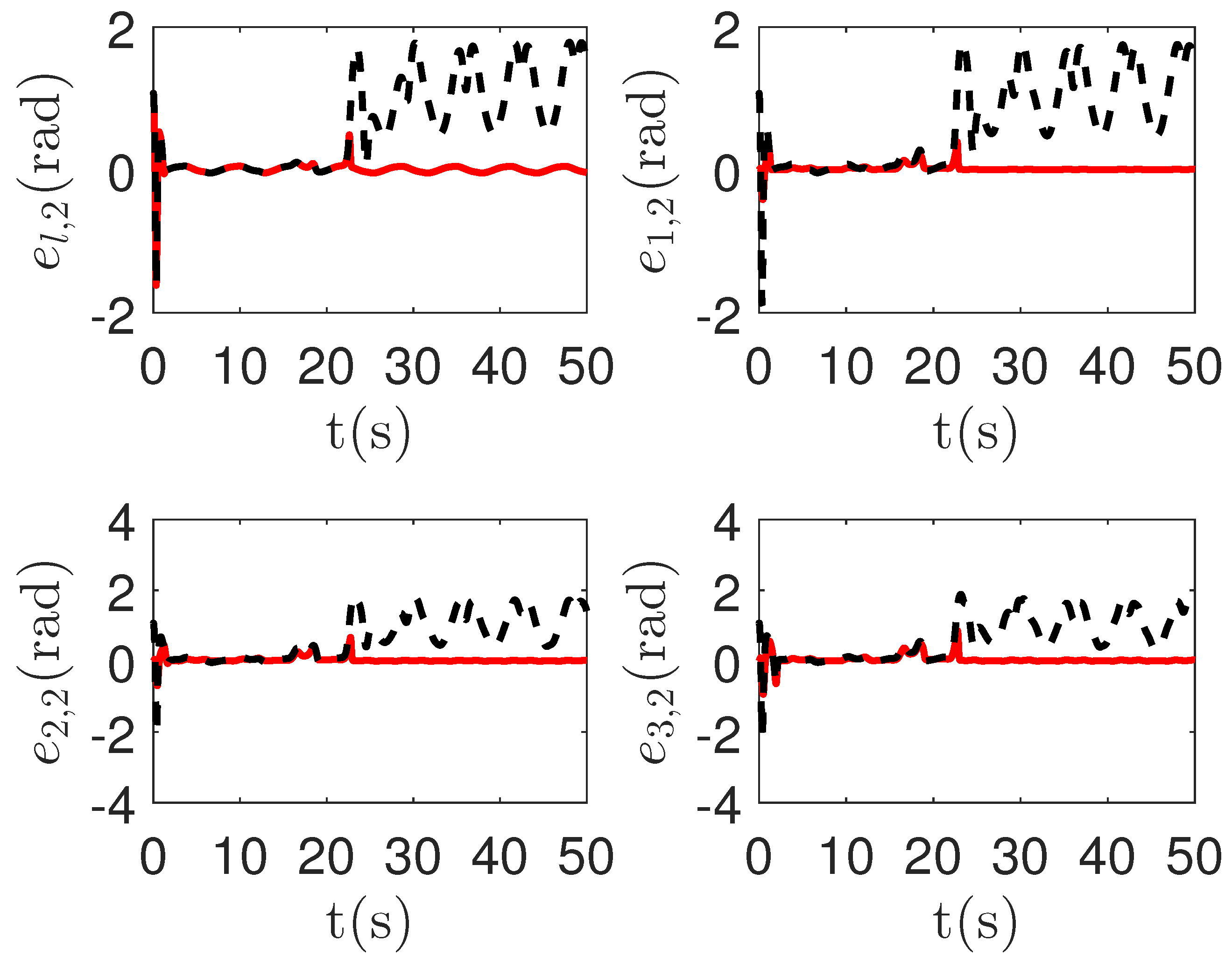
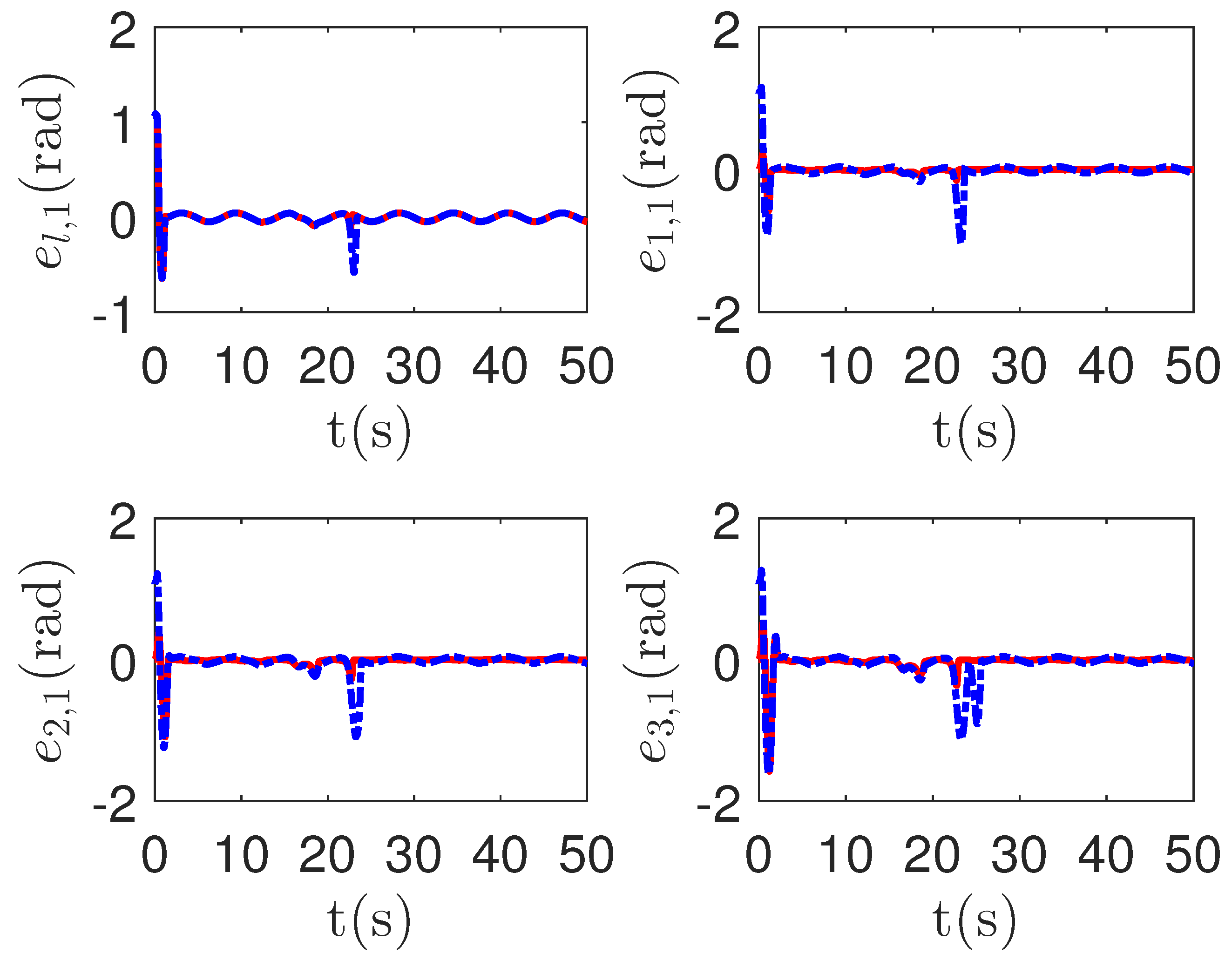
 : The proposed method;: The active fault-tolerant control method with passive fault detection [68].
 : The proposed method;: The active fault-tolerant control method with passive fault detection [68].
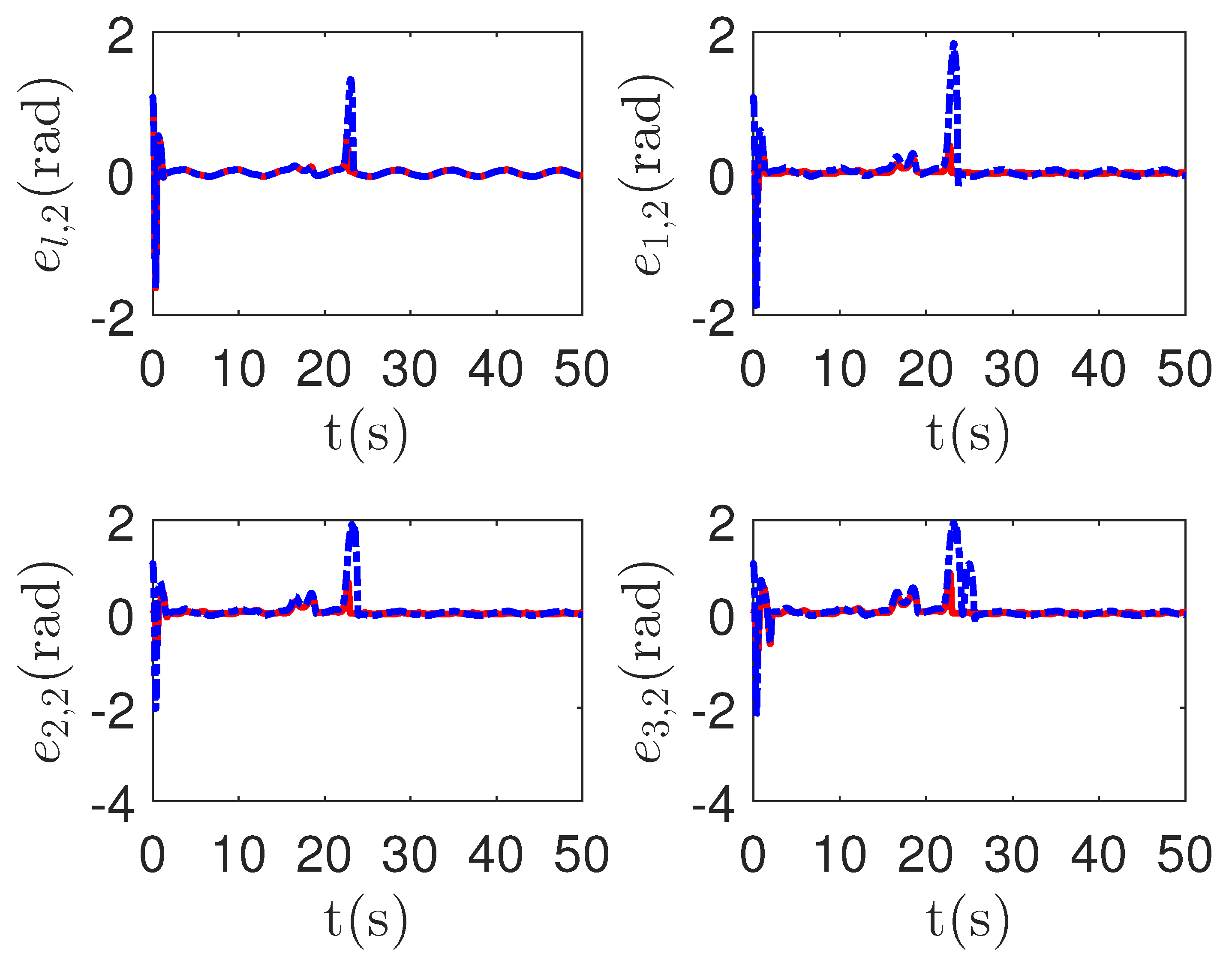
 : The proposed method;: The active fault-tolerant control method with passive fault detection [68].
 : The proposed method;: The active fault-tolerant control method with passive fault detection [68].
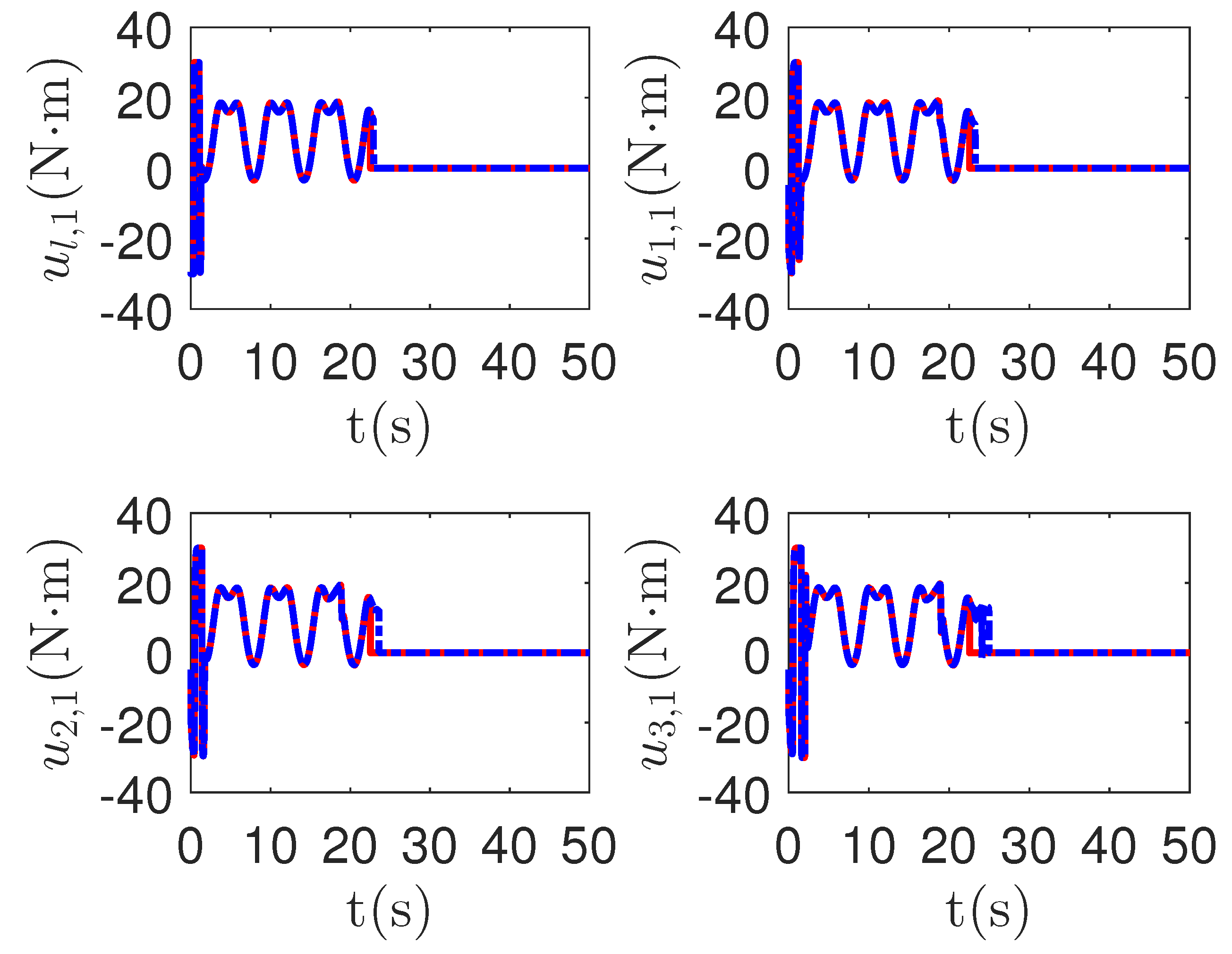
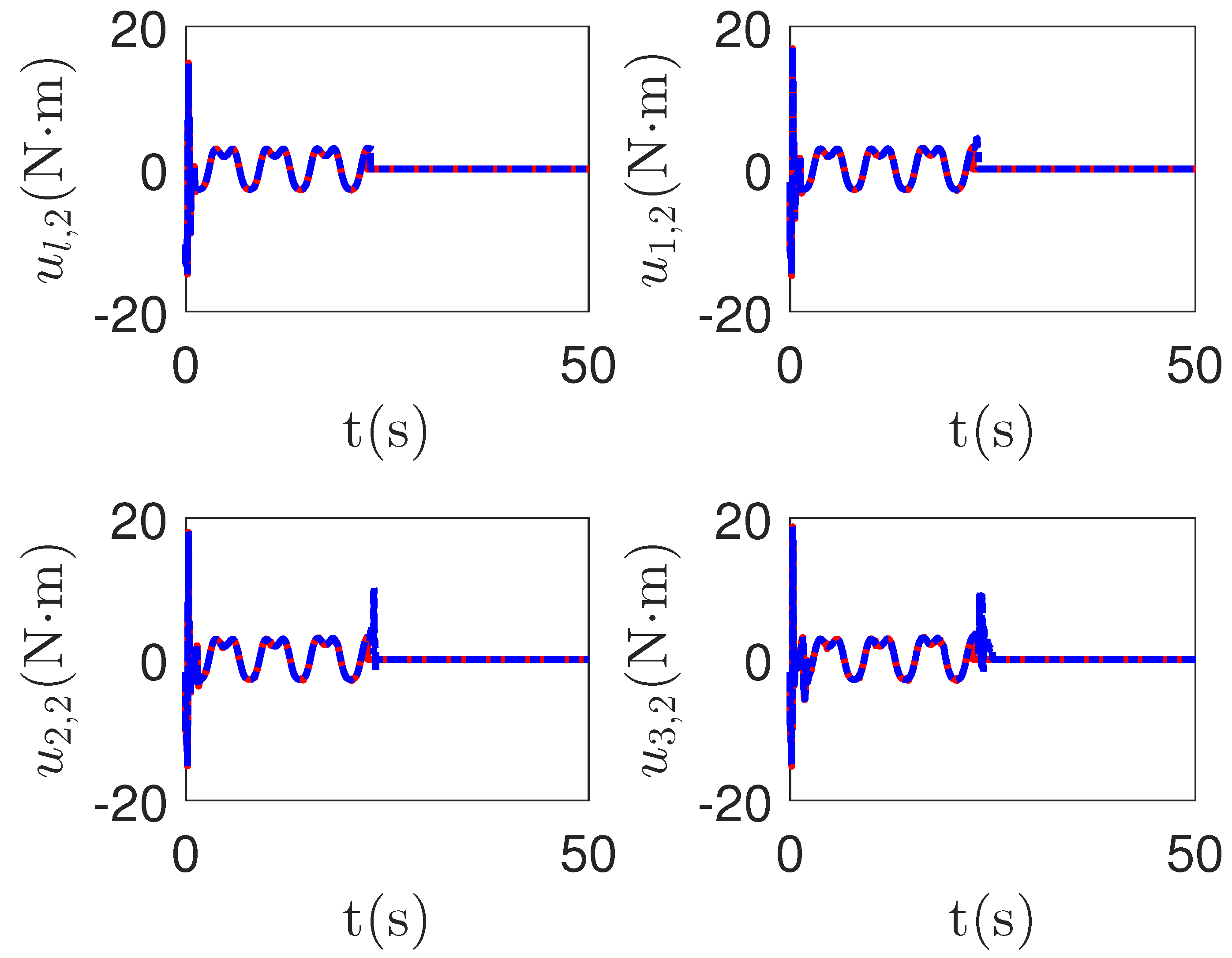
 : The proposed method;: The active fault-tolerant control method with passive fault detection [68].

Disclaimer/Publisher’s Note: The statements, opinions and data contained in all publications are solely those of the individual author(s) and contributor(s) and not of MDPI and/or the editor(s). MDPI and/or the editor(s) disclaim responsibility for any injury to people or property resulting from any ideas, methods, instructions or products referred to in the content. |
© 2023 by the authors. Licensee MDPI, Basel, Switzerland. This article is an open access article distributed under the terms and conditions of the Creative Commons Attribution (CC BY) license (https://creativecommons.org/licenses/by/4.0/).
Share and Cite
Yan, W.; Tu, H.; Qin, P.; Zhao, T. Interval Type-II Fuzzy Fault-Tolerant Control for Constrained Uncertain 2-DOF Robotic Multi-Agent Systems with Active Fault Detection. Sensors 2023, 23, 4836. https://doi.org/10.3390/s23104836
Yan W, Tu H, Qin P, Zhao T. Interval Type-II Fuzzy Fault-Tolerant Control for Constrained Uncertain 2-DOF Robotic Multi-Agent Systems with Active Fault Detection. Sensors. 2023; 23(10):4836. https://doi.org/10.3390/s23104836
Chicago/Turabian StyleYan, Wen, Haiyan Tu, Peng Qin, and Tao Zhao. 2023. "Interval Type-II Fuzzy Fault-Tolerant Control for Constrained Uncertain 2-DOF Robotic Multi-Agent Systems with Active Fault Detection" Sensors 23, no. 10: 4836. https://doi.org/10.3390/s23104836
APA StyleYan, W., Tu, H., Qin, P., & Zhao, T. (2023). Interval Type-II Fuzzy Fault-Tolerant Control for Constrained Uncertain 2-DOF Robotic Multi-Agent Systems with Active Fault Detection. Sensors, 23(10), 4836. https://doi.org/10.3390/s23104836