
Brain Magnetic Resonance Imaging Classification Using Deep Learning Architectures with Gender and Age

 , ,
, ,  ,
,  and
and
Abstract
:1. Introduction
1.1. Motivation
1.2. Our Contributions
- Figshare [9], Brainweb [10], and Radiopaedia [11] datasets are readily available online and can be used to classify brain MRI as normal or abnormal. We have taken all these datasets to create a heterogeneous combination of data that address the heterogeneity issue. A dataset from the same source is used for the majority of studies in brain-related diagnosis. This form of heterogeneity has never been explored before, but it could be the beginning of correctly distinguishing images from different sources.
- Using higher attributes is always more informative with a higher expectancy of reliable and efficient results. Here, work based on age and gender is considered as an initiative to determine whether these can be helpful in further automated diagnosis. It is inspired by the paper given in [12,13]. In addition to employing various data to classify patients as normal or abnormal, Radiopaedia datasets are used to classify patients by age and gender.
- To categorize normal (absence of tumor) and abnormal (presence of tumor) images, two proposed CNN-based methodologies are applied. One is a model that is inspired from LeNet and the other is a Deep Neural Network based method. These proposed models are fast and more superficial compared to other comparable deep learning methods.
- Two alternative deep learning-based classifiers, LeNet and ResNet, are incorporated in addition to the proposed methodology for classification. During their reign, these two models were used for classification and had a significant impact. They are utilized because they are not as deep as VGG19, MobileNet, Inception, and other state-of-the-art deep learning approaches, which are not ideal for our data as they are not massive and could lead to erroneous results and computational expense. To classify normal and abnormal images, the results are compared with Support Vector Machine and AlexNet, which were previously used to classify normal and abnormal images.
- Compared to traditional SVM (82% using age and gender attributes and 77% using heterogenous data without any attributes), the parameters used in this paper are higher with better results and accuracy (88% using age and gender attributes and 80% using heterogenous data). While comparing to AlexNet, the depth and number of convolutions are lesser in the proposed method, making it simpler with more efficient computation time. AlexNet obtained an accuracy of 64% using age and gender attributes and 65% using heterogenous data without any attributes.
- In this paper, data are not equally distributed for each group using age and gender. Data are unbalanced data, and cross-validation is used to solve this issue. This work is not clinically proven or tested, but it is performed to check the capability of a few deep-learning methodologies, mainly spatial CNN. This model might not work or perform well under different clinical settings, as data are obtained from online sources.
1.3. Organization of the Paper
2. Related Works
2.1. A Brief Description on Existing Techniques Used in Classification of MRI into Normal and Abnormal
2.1.1. Support Vector Machine (SVM)
2.1.2. AlexNet
3. Classification of Brain MRI Images Using Deep Learning Architectures
3.1. Proposed Methodology
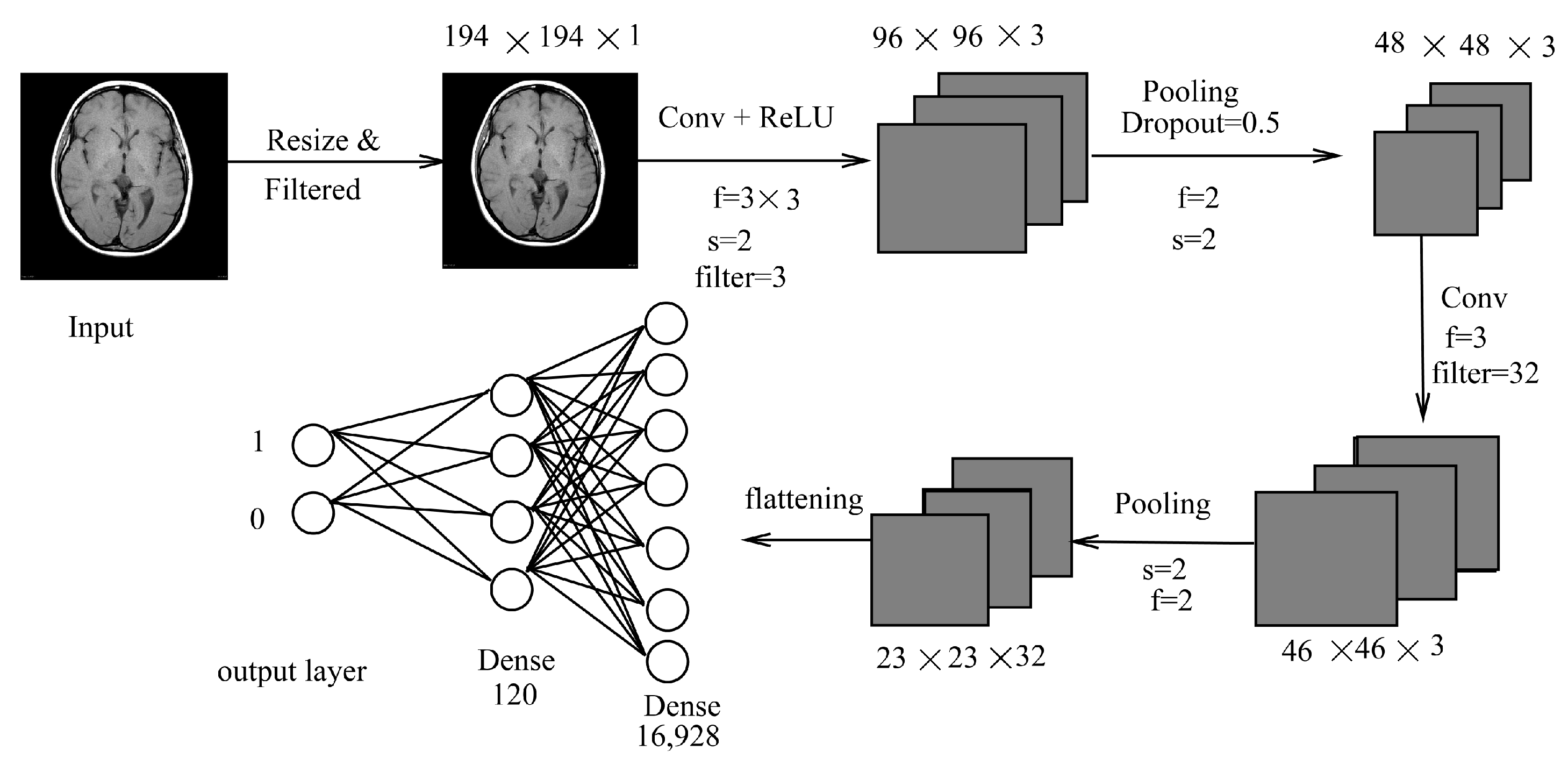
3.1.1. LeNet Inspired Model
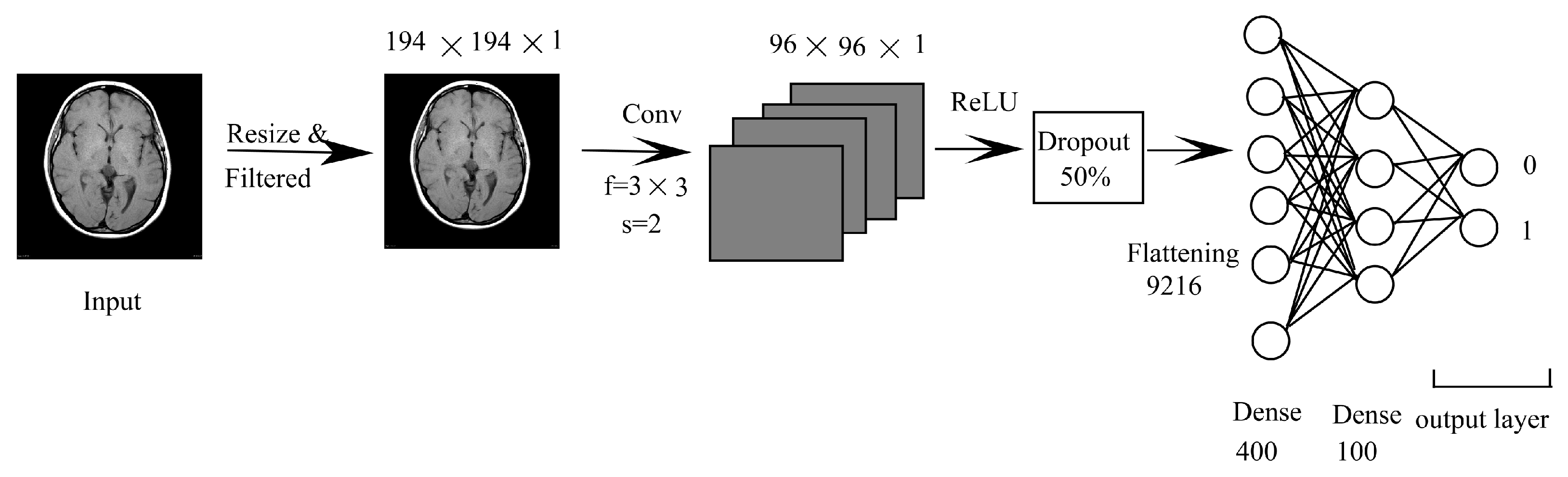
3.1.2. CNN Combined with DNN (CNN-DNN)
3.2. LeNet
3.3. ResNet50 (Transfer Learning)
4. Experimental Results
4.1. Performance Metrics
4.2. Normal or Abnormal Classification
4.3. Range Based Classification
4.4. Statistical Significance Test
4.5. Benefits and Drawbacks of Our Methods
4.6. Summary
- Using age and gender as attributes with a range of ages is more informative, as it involves higher attributes and, as a result, is less biased. This helps in effective and efficient analysis of the brain and its abnormalities.
- In most instances, classification into normal or abnormal without using age and gender as attributes yields less accurate results. This shows that using age and gender attributes is relevant and valuable in the classification of brains into normal or abnormal class.
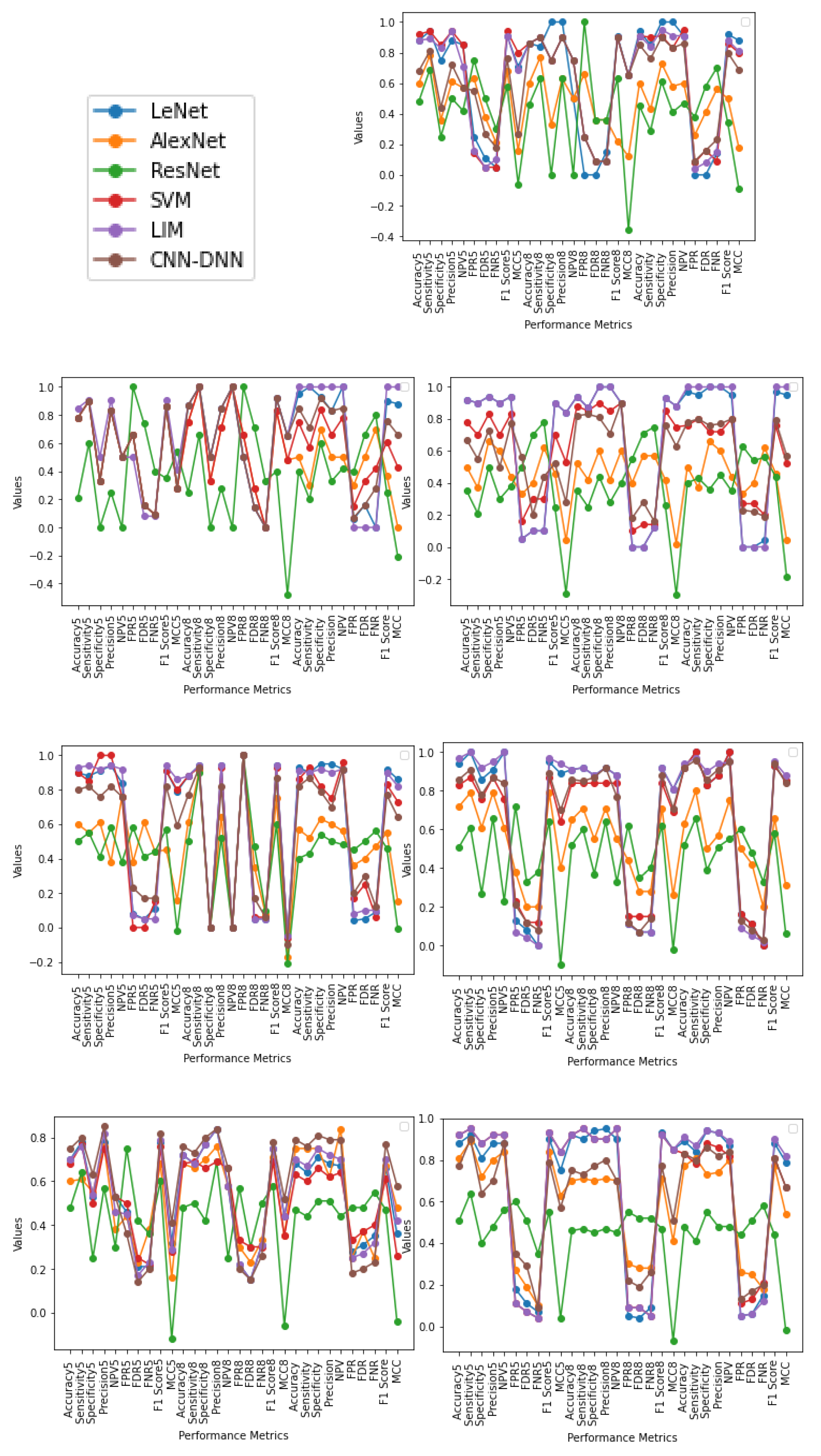
- The pattern obtained in the case of Female (20–70) and Male + Female (10–80) yielded better results than that of other age range in almost all methodologies which signifies that using age and gender as attributes are essential and can help in better classification of a tumor. Furthermore, the same applies in the case of Male + Female, where age acts as a significant factor in providing an efficient and reliable classification where, taking gender as a factor, the result is accurate in most cases.
- This can be interpreted as though the output is better differentiated when both male and female are taken as separate inputs. It can be observed that assumptions of the same age range of the same gender are likely to have similar patterns, as output is better in most cases. This is because brain volume varies by 50% even in the group of the same age and varies differently for different genders [7,8]. Gender as a factor has shown a more promising result.
- From performance metrics and ANOVA tests, using gender can be considered a relevant factor as the pattern and output are better when taking Male or Female as a separate input; also, when combining the gender of all ages, the pattern does not change much, which can imply that gender is a dominating factor over age. The pattern obtained in the case of Male (10–80) and Female (10–80) does not provide a better result than when combining the two genders in all methodologies (except in a few cases using statistical test), which shows that similarities between males and females could be differentiated better using gender as an attribute. Using both age and gender attributes thus acts as an essential factor in providing better accuracy in diagnosis as a whole.
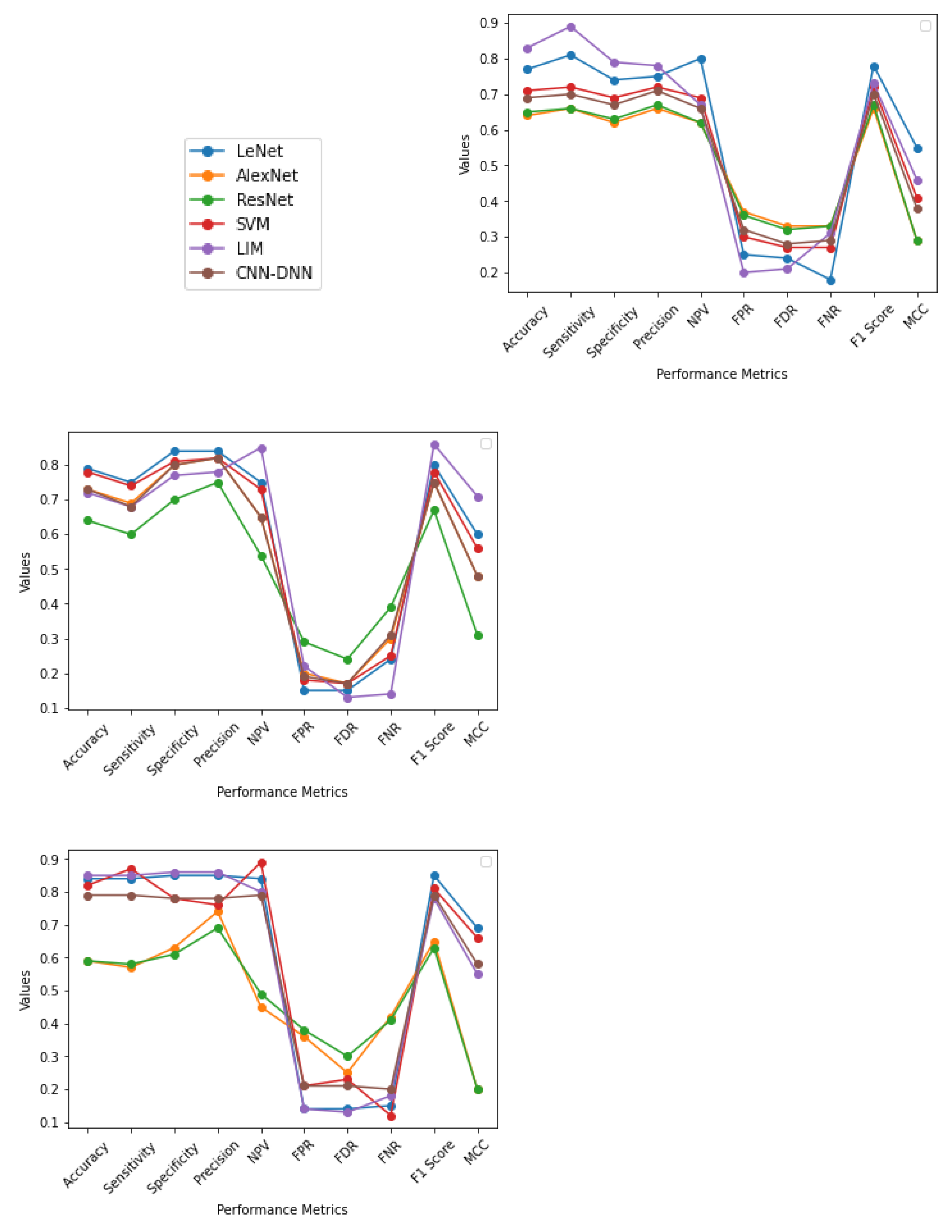
- In most cases, the output is better when CNN-based methodologies are applied instead of the SVM method. In several cases, LIM is in first or second place. On the other hand, CNN-DNN can be comparable to SVM in output provided by the generalization and k fold cross-validation approaches. This shows that deep learning methodologies have the potential to achieve reliable results through further experiments in the future. The deep learning model has more layers and provides finer details at a deeper level about the images, which act as a tool for a better prognosis.
- Although gender is more dominating than age as per our utilized data and result, it is not enough to say whether any variable is statistically significant based on the ANOVA test. On the other hand, the model (LIM) is statistically significant. Using higher variables as a relevant factor is reasonable based on performance metrics and the ANOVA test.
5. Conclusions and Future Work
Author Contributions
Funding
Institutional Review Board Statement
Informed Consent Statement
Data Availability Statement
Conflicts of Interest
References
- Brain Anatomy. Available online: https://emedicine.medscape.com/article/1898830-overview (accessed on 20 July 2018).
- Anatomy of the Brain. Available online: https://mayfieldclinic.com/pe-Anatbrain.htm (accessed on 20 July 2018).
- Brain. Available online: https://www.innerbody.com/image/nerv02.html (accessed on 18 July 2018).
- Brain Cancer. Available online: https://www.webmd.com/cancer/brain-cancer/default.htm (accessed on 18 July 2018).
- Brain Tumor: Diagnosis. Available online: https://www.cancer.net/cancer-types/brain-tumor/diagnosis (accessed on 18 July 2018).
- Burje, S.; Rungta, S.; Shukla, A. Detection and classification of MRI brain images for head/brain injury using soft computing techniques. Res. J. Pharm. Technol. 2017, 10, 715–720. [Google Scholar] [CrossRef]
- Giedd, J.N. The teen brain: Insights from neuroimaging. J. Adolesc. Health 2008, 42, 335–343. [Google Scholar] [CrossRef] [PubMed]
- Finlay, B.L.; Darlington, R.B.; Nicastro, N. Developmental structure in brain evolution. Behav. Brain Sci. 2001, 24, 263–308. [Google Scholar] [CrossRef] [Green Version]
- Figshare. Available online: https://figshare.com/ (accessed on 20 July 2018).
- BrainWeb: Simulated Brain Database. Available online: https://brainweb.bic.mni.mcgill.ca/brainweb/ (accessed on 20 July 2018).
- Radiopaedia. Available online: https://radiopaedia.org/cases (accessed on 12 July 2018).
- Brown, T.T. Individual differences in human brain development. Wiley Interdiscip. Rev. Cogn. Sci. 2017, 8, 1–8. [Google Scholar] [CrossRef] [PubMed]
- Xin, J.; Zhang, Y.; Tang, Y.; Yang, Y. Brain differences between men and women: Evidence from deep learning. Front. Neurosci. 2019, 13, 185. [Google Scholar] [CrossRef] [Green Version]
- Rajesh, T.; Malar, R.S.M. Rough set theory and feed forward neural network based brain tumor detection in magnetic resonance images. In Proceedings of the International Conference on Advanced Nanomaterials and Emerging Engineering Technologies (ICANMEET), Chennai, India, 24–26 July 2013; pp. 240–244. [Google Scholar]
- Taie, S.; Ghonaim, W. CSO-based algorithm with support vector machine for brain tumor’s disease diagnosis. In Proceedings of the IEEE International Conference on Pervasive Computing and Communications Workshops (Per-Com Workshops), Pisa, Italy, 21–25 March 2017; pp. 183–187. [Google Scholar]
- Balasubramanian, C.; Sudha, B. Comparative Study of De-Noising, Segmentation, Feature Extraction, Classification Techniques for Medical Images. Int. J. Innov. Res. Sci. Eng. Technol. 2014, 3, 1194–1199. [Google Scholar]
- Nelly, G.; Montseny, E.; Sobrevilla, P. State of the art survey on MRI brain tumor segmentation. Magn. Reson. Imaging 2013, 31, 1426–1438. [Google Scholar]
- Al-Badarneh, A.; Najadat, H.; Alraziqi, A.M. A classifier to detect tumor disease in MRI brain images. In Proceedings of the 2012 International Conference on Advances in Social Networks Analysis and Mining (ASONAM), Istanbul, Turkey, 26–29 August 2012; pp. 784–787. [Google Scholar]
- Singh, D.A. Review of Brain Tumor Detec- tion from MRI Images. In Proceedings of the 3rd International Conference on Computing for Sustainable Global Development (INDIACom), New Delhi, India, 16–18 March 2016; pp. 3997–4000. [Google Scholar]
- Mohsen, H.; El-Dahshan, E.; Salem, A.M. A machine learning technique for MRI brain images. In Proceedings of the International Conference on Informatics and Systems (BIO-161), Cairo, Egypt, 20 March–14 May 2012. [Google Scholar]
- Pereira, S.; Pinto, A.; Alves, V.; Silva, C.A. Brain Tumor Segmentation Using Convolutional Neural Networks in MRI Images. IEEE Trans. Med. Imaging 2016, 35, 1240–1251. [Google Scholar] [CrossRef] [PubMed]
- Kamnitsas, K.; Ledig, C.; Newcombe, V.F.; Simpson, J.P.; Kane, A.D.; Menon, D.K.; Rueckert, D.; Glocker, B. Multi-scale 3D CNN with Fully Con- nected CRF for Accurate Brain Lesion Segmentation. Med. Image Anal. 2017, 36, 61–78. [Google Scholar] [CrossRef]
- Roy, S.; Bandyopadhyay, S.K. Brain Tumor Classification and Performance Analysis. Int. J. Eng. Sci. 2018, 8, 18541–18545. [Google Scholar]
- Krishnammal, P.M.; Raja, S.S. Convolutional Neural Network based Image Classification and Detection of Abnormalities in MRI Brain Images. In Proceedings of the International Conference on Communication and Signal Processing (ICCSP), Kuala Lumpur, Malaysia, 4–6 April 2019; pp. 0548–0553. [Google Scholar]
- Hanwat, S.; Jayaraman, C. Convolutional Neural Network for Brain Tumor Analysis Using MRI Images. Int. J. Eng. Technol. 2019, 11, 67–77. [Google Scholar] [CrossRef] [Green Version]
- Ramachandran, R.P.R.; Mohanapriya, R.; Banupriya, V. A Spearman Algorithm Based Brain Tumor Detection Using CNN Classifier for MRI Images. Int. J. Eng. Adv. Technol. (IJEAT) 2019, 8, 394–398. [Google Scholar]
- Badža, M.M.; Barjaktarović, M.Č. Classification of Brain Tumors from MRI Images Using a Convolutional Neural Network. Appl. Sci. 2020, 10, 1999. [Google Scholar] [CrossRef] [Green Version]
- Lee, J.G.; Jun, S.; Cho, Y.W.; Lee, H.; Kim, G.B.; Seo, J.B.; Kim, N. Deep learning in medical imaging: General overview. Korean J. Radiol. 2017, 18, 570–584. [Google Scholar] [CrossRef] [Green Version]
- Li, M.; Kuang, L.; Xu, S.; Sha, Z. Brain tumor detection based on multimodal information fusion and convolutional neural network. IEEE Access 2019, 7, 180134–180146. [Google Scholar] [CrossRef]
- Hamid, M.A.; Khan, N.A. Investigation and Classification of MRI Brain Tumors Using Feature Extraction Technique. J. Med. Biol. Eng. 2020, 40, 307–317. [Google Scholar] [CrossRef]
- Dogra, J.; Jain, S.; Sood, M. Gradient-based kernel selection technique for tumour detection and extraction of medical images using graph cut. IET Image Process. 2020, 14, 84–93. [Google Scholar] [CrossRef]
- Kalaiselvi, K.; Karthikeyan, C.; Shenbaga Devi, M.; Kalpana, C. Improved Classification of Brain Tumor in MR Images using RNN Classification Framework. Int. J. Innov. Technol. Explor. Eng. (IJITEE) 2020, 9, 1098–1101. [Google Scholar]
- Suganthe, R.C.; Revathi, G.; Monisha, S.; Pavithran, R. Deep Learning Based Brain Tumor Classification Using Magnetic Resonance Imaging. J. Crit. Rev. 2020, 7, 347–350. [Google Scholar]
- Kulkarni, S.M.; Sundari, G. Brain MRI Classification using Deep Learning Algorithm. Int. J. Eng. Adv. Technol. (IJEAT) 2020, 9, 1226–1231. [Google Scholar] [CrossRef]
- Mohsen, H.; El-Dahshan, E.S.A.; El-Horbaty, E.S.M.; Salem, A.B.M. Classification using deep learning neural networks for brain tumors. Future Comput. Inform. J. 2018, 3, 68–71. [Google Scholar] [CrossRef]
- Zhang, J.; Xie, Y.; Wu, Q.; Xia, Y. Medical image classification using synergic deep learning. Med. Image Anal. 2019, 54, 10–19. [Google Scholar] [CrossRef] [PubMed]
- Kumar Mallick, P.; Ryu, S.H.; Satapathy, S.K.; Mishra, S.; Nguyen, G.N.; Tiwari, P. Brain MRI image classification for cancer detection using deep wavelet autoencoder-based deep neural network. IEEE Access 2019, 7, 46278–46287. [Google Scholar] [CrossRef]
- Khan, H.A.; Jue, W.; Mushtaq, M.; Mushtaq, M.U. Brain tumor classification in MRI image using convolutional neural network. Math. Biosci. Eng. 2020, 17, 6203–6216. [Google Scholar] [CrossRef]
- Latha, R.S.; Sreekanth, G.R.; Akash, P.; Dinesh, B. Brain Tumor Classification using SVM and KNN Models for Smote Based MRI Images. J. Crit. Rev. 2020, 7, 1–4. [Google Scholar]
- Kumar, P.; VijayKumar, B. Brain Tumor MRI Segmentation and Classification Using Ensemble Classifier. Int. J. Recent Technol. Eng. (IJRTE) 2018, 8, 244–252. [Google Scholar]
- International MICCAI BraTS Challenge. 1-578. 2018. Available online: https://www.cbica.upenn.edu/sbia/Spyridon.Bakas/MICCAI_BraTS/MICCAI_BraTS_2018_proceedings_shortPapers.pdf (accessed on 20 July 2018).
- Ramaswamy Reddy, A.; Prasad, E.V.; Reddy, L.S.S. Comparative analysis of brain tumor detection using different segmentation techniques. Int. J. Comput. Appl. 2013, 82, 0975–8887. [Google Scholar]
- Krizhevsky, A.; Sutskever, I.; Hinton, G.E. Imagenet classification with deep convolutional neural networks. Adv. Neural Inf. Process. Syst. 2012, 25, 1097–1105. [Google Scholar] [CrossRef]
- Magnetic Resonance Imaging (MRI) of the Brain and Spine: Basics. Available online: https://case.edu/med/neurology/NR/MRI%20Basics.htm (accessed on 20 July 2018).
- Understanding Binary Cross-Entropy/Log Loss: A Visual Explanation. Available online: https://towardsdatascience.com/understanding-binary-cross-entropy-log-loss-a-visual-explanation-a3ac6025181a (accessed on 18 July 2018).
- LeCun, Y.; Bengio, Y.; Hinton, G. Deep learning. Nature 2015, 521, 436–444. [Google Scholar] [CrossRef]
- Simonyan, K.; Zisserman, A. Very deep convolutional networks for large-scale image recognition. In Proceedings of the Computer Vision and Pattern Recognition, Columbus, OH, USA, 24–27 June 2014; pp. 1–14. [Google Scholar]
- Huang, G.; Liu, Z.; Weinberger, K.Q.; van der Maaten, L. Densely connected convolutional networks. In Proceedings of the Computer Vision and Pattern Recognition, Salt Lake City, UT, USA, 18–22 June 2018; pp. 1097–1105. [Google Scholar]
- Suhag, S.; Saini, L.M. Automatic Brain Tumor Detection and Classification using SVM Classifier. Int. J. Adv. Sci. Eng. Technol. 2015, 3, 119–123. [Google Scholar]
- Demšar, J. Statistical comparisons of classifiers over multiple data sets. J. Mach. Learn. Res. 2006, 7, 1–30. [Google Scholar]


| Paper and Year | Method | Classification | Dataset Used | Accuracy (%) |
|---|---|---|---|---|
| Al-Baderneh et al. (2012) [18] | NN and KNN | Normal/Abnormal | 275 images | 100 and 98.92 |
| Rajesh et al. (2013) [14] | Feed Forward Neural Network | Normal/Abnormal | 20 images | 90 |
| Taie et al. (2017) [15] | SVM | 80, 100, and 150 images | 90.89 and 100 | |
| krishnammal et al. (2019) [24] | AlexNet | Benign/Malignant | Not mention | 100 |
| Hanwat et al. (2019) [25] | CNN | Benign/Malignant/ Normal | 94 images | 71 |
| Hamid et al. (2020) [30] | DWT, GLM, and SVM | Benign/Malignant | Dicom images | 95 |
| Kulkarni et al. (2020) [34] | AlexNet | Benign/Malignant | 75 Benign and 75 Malignant images | 98.44 (F measure) |
| Parameter Name | LeNet | AlexNet | ResNet | LIM | CNN-DNN |
|---|---|---|---|---|---|
| Number of convolution layer | 2 | 5 | 48 | 2 | 1 |
| Number of pooling layer | 2 () | 3 () | 24 () | 2 () | Nil |
| Depth | 32 | 96 | 512 | 32 | 3 |
| Filter size | , , | , | |||
| Loss function | binary crossentropy | binary crossentropy | binary crossentropy | binary crossentropy | binary crossentropy |
| Classifier | Sigmoid | Softmax | Softmax | Softmax | Sigmoid |
| Number of Dropout | 3 | 3 | 10 | 2 | 2 |
| Dropout rate | 0.5 | 0.5 | 0.5 | 0.5 | 0.5 |
| Activation Function | tanH | ReLU | ReLU | ReLU | Sigmoid |
| Optimizer | Sgd | Sgd | Adam | Adam | Adam |
| Model type | cascade | cascade | cascade | cascade | cascade |
| No. | Performance Metric | Description |
|---|---|---|
| 1 | Accuracy | Accuracy is a measurement that gives the correctness of classification and loss is a measure indicating that how well a model behaves after every iteration. |
| 2 | Precision | The fraction of true positives (TP) from the total amount of relevant result. Precision = TP/(TP + FP). |
| 3 | Recall (Sensitivity) | The fraction of true positives from the total amount of TP and FN. Recall = TP/(TP + FN). |
| 4 | F1 Score | The harmonic mean of Precision and Recall given by the following formula: F1 = 2 ∗ (TP ∗ FP)/(TP + FP) |
| 5 | Specificity | Specificity = TN/(FP + TN) |
| 6 | Negative Predictive Value | NPV = TN/(TN + FN) |
| 7 | False Positive Rate | FPR = FP/(FP + TN) |
| 8 | False Discovery Rate | FDR = FP (FP + TP) |
| 9 | False Negative Rate | FNR = FN/(FN + TP) |
| 10 | Matthews Correlation Coefficient | TP ∗ TN − FP ∗ FN/sqrt((TP + FP) ∗ (TP + FN) ∗ (TN + FP) ∗ (TN + FN)) |
| Methods | Phase | Parameters | Five-Fold | Eight-Fold | Generalization | Methods | Phase | Parameters | 5 Fold | Eight-Fold | Generalization |
|---|---|---|---|---|---|---|---|---|---|---|---|
| Accuracy | 0.79 | 0.82 | 0.83 | Accuracy | 0.80 | 0.81 | 0.83 | ||||
| Training | Loss | 0.44 | 0.37 | 0.42 | Training | Loss | NA | NA | NA | ||
| Accuracy | 0.77 | 0.79 | 0.84 | Accuracy | 0.71 | 0.78 | 0.82 | ||||
| Sensitivity | 0.81 | 0.75 | 0.84 | Sensitivity | 0.72 | 0.74 | 0.87 | ||||
| Specificity | 0.74 | 0.84 | 0.85 | Specificity | 0.69 | 0.81 | 0.78 | ||||
| Precision | 0.75 | 0.84 | 0.85 | Precision | 0.72 | 0.82 | 0.76 | ||||
| NPV | 0.80 | 0.75 | 0.84 | NPV | 0.69 | 0.73 | 0.89 | ||||
| FPR | 0.25 | 0.15 | 0.14 | FPR | 0.30 | 0.18 | 0.21 | ||||
| FDR | 0.24 | 0.15 | 0.14 | FDR | 0.27 | 0.17 | 0.23 | ||||
| FNR | 0.18 | 0.24 | 0.15 | FNR | 0.27 | 0.25 | 0.12 | ||||
| F1 Score | 0.78 | 0.80 | 0.85 | F1 Score | 0.72 | 0.78 | 0.81 | ||||
| MCC | 0.55 | 0.60 | 0.69 | MCC | 0.41 | 0.56 | 0.66 | ||||
| LeNet | Testing | Loss | 0.42 | 0.43 | 0.40 | SVM | Testing | Loss | NA | NA | NA |
| Accuracy | 0.97 | 0.73 | 0.55 | Accuracy | 0.81 | 0.68 | 0.90 | ||||
| Training | Loss | 0.07 | 0.77 | 5.54 | Training | Loss | 0.41 | 0.36 | 0.20 | ||
| Accuracy | 0.64 | 0.73 | 0.59 | Accuracy | 0.83 | 0.72 | 0.85 | ||||
| Sensitivity | 0.66 | 0.69 | 0.57 | Sensitivity | 0.89 | 0.68 | 0.85 | ||||
| Specificity | 0.62 | 0.80 | 0.63 | Specificity | 0.79 | 0.77 | 0.86 | ||||
| Precision | 0.66 | 0.82 | 0.74 | Precision | 0.78 | 0.78 | 0.86 | ||||
| NPV | 0.62 | 0.65 | 0.45 | NPV | 0.67 | 0.85 | 0.80 | ||||
| FPR | 0.37 | 0.20 | 0.36 | FPR | 0.20 | 0.22 | 0.14 | ||||
| FDR | 0.33 | 0.17 | 0.25 | FDR | 0.21 | 0.13 | 0.13 | ||||
| FNR | 0.33 | 0.30 | 0.42 | FNR | 0.31 | 0.14 | 0.18 | ||||
| F1 Score | 0.66 | 0.75 | 0.65 | F1 Score | 0.73 | 0.86 | 0.78 | ||||
| MCC | 0.29 | 0.48 | 0.20 | MCC | 0.46 | 0.71 | 0.55 | ||||
| AlexNet | Testing | Loss | 1.33 | 0.95 | 5.94 | LIM | Testing | Loss | 0.39 | 0.60 | 0.39 |
| Accuracy | 0.67 | 0.70 | 0.65 | Accuracy | 0.81 | 0.80 | 0.81 | ||||
| Training | Loss | 0.70 | 0.76 | 0.83 | Training | Loss | 0.49 | 0.50 | 0.55 | ||
| Accuracy | 0.65 | 0.64 | 0.59 | Accuracy | 0.69 | 0.73 | 0.79 | ||||
| Sensitivity | 0.66 | 0.60 | 0.58 | Sensitivity | 0.70 | 0.68 | 0.79 | ||||
| Specificity | 0.63 | 0.70 | 0.61 | Specificity | 0.67 | 0.80 | 0.78 | ||||
| Precision | 0.67 | 0.75 | 0.69 | Precision | 0.71 | 0.82 | 0.78 | ||||
| NPV | 0.62 | 0.54 | 0.49 | NPV | 0.66 | 0.65 | 0.79 | ||||
| FPR | 0.36 | 0.29 | 0.38 | FPR | 0.32 | 0.19 | 0.21 | ||||
| FDR | 0.32 | 0.24 | 0.30 | FDR | 0.28 | 0.17 | 0.21 | ||||
| FNR | 0.33 | 0.39 | 0.41 | FNR | 0.29 | 0.31 | 0.20 | ||||
| F1 Score | 0.67 | 0.67 | 0.63 | F1 Score | 0.70 | 0.75 | 0.79 | ||||
| MCC | 0.29 | 0.31 | 0.20 | MCC | 0.38 | 0.48 | 0.58 | ||||
| ResNet | Testing | Loss | 0.74 | 0.64 | 0.83 | CNNDNN | Testing | Loss | 0.55 | 0.56 | 0.61 |
| Age and Gender | Approach | Training | Testing | |||||||||||
|---|---|---|---|---|---|---|---|---|---|---|---|---|---|---|
| Accuracy | Loss | Accuracy | Sensitivity | Specificity | Precision | NPV | FPR | FDR | FNR | F1 Score | MCC | Loss | ||
| Male (20–70) | Five-fold | 0.93 | 0.28 | 0.88 | 0.94 | 0.75 | 0.88 | 0.85 | 0.25 | 0.11 | 0.05 | 0.91 | 0.71 | 0.38 |
| Eight-fold | 0.95 | 0.72 | 0.86 | 0.84 | 1 | 1 | 0.5 | 0 | 0 | 0.15 | 0.91 | 0.65 | 0.43 | |
| Gen | 0.93 | 0.12 | 0.94 | 0.85 | 1 | 1 | 0.91 | 0 | 0 | 0.14 | 0.92 | 0.88 | 0.10 | |
| Female (50–70) | Five-fold | 0.92 | 0.41 | 0.78 | 0.90 | 0.33 | 0.83 | 0.50 | 0.66 | 0.16 | 0.09 | 0.86 | 0.28 | 0.43 |
| Eight-fold | 1 | 0.12 | 0.87 | 1 | 0.50 | 0.85 | 1 | 0.50 | 0.14 | 0 | 0.92 | 0.65 | 0.48 | |
| Gen | 1 | 0.09 | 0.95 | 1 | 0.93 | 0.83 | 1 | 0.06 | 0.16 | 0 | 0.90 | 0.88 | 0.09 | |
| Female (20–70) | Five-fold | 0.96 | 0.15 | 0.92 | 0.90 | 0.94 | 0.90 | 0.94 | 0.05 | 0.1 | 0.1 | 0.90 | 0.84 | 0.14 |
| Eight-fold | 0.96 | 0.14 | 0.94 | 0.87 | 1 | 1 | 0.90 | 0 | 0 | 0.12 | 0.93 | 0.88 | 0.15 | |
| Gen | 0.92 | 0.19 | 0.97 | 0.95 | 1 | 1 | 0.95 | 0 | 0 | 0.04 | 0.97 | 0.95 | 0.15 | |
| Male (10–80) | Five-fold | 0.89 | 0.37 | 0.90 | 0.88 | 0.91 | 0.94 | 0.84 | 0.08 | 0.05 | 0.11 | 0.91 | 0.79 | 0.43 |
| Eight-fold | 0.88 | 0.27 | 0.88 | 0.94 | 0 | 0.94 | 0 | 1 | 0.05 | 0.05 | 0.94 | −0.05 | 0.21 | |
| Gen | 0.88 | 0.20 | 0.93 | 0.90 | 0.95 | 0.95 | 0.92 | 0.04 | 0.05 | 0.09 | 0.92 | 0.86 | 0.17 | |
| Female (10–80) | Five-fold | 0.94 | 0.21 | 0.94 | 1 | 0.86 | 0.91 | 1 | 0.13 | 0.08 | 0 | 0.95 | 0.89 | 0.20 |
| Eight-fold | 1 | 0.09 | 0.91 | 0.92 | 0.88 | 0.92 | 0.88 | 0.11 | 0.07 | 0.07 | 0.92 | 0.81 | 0.18 | |
| Gen | 0.95 | 0.14 | 0.92 | 1 | 0.83 | 0.88 | 1 | 0.16 | 0.11 | 0 | 0.93 | 0.85 | 0.14 | |
| Male + Female (20–70) | Five-fold | 0.70 | 0.57 | 0.70 | 0.78 | 0.53 | 0.78 | 0.53 | 0.46 | 0.21 | 0.21 | 0.78 | 0.32 | 0.52 |
| Eight-fold | 0.76 | 0.51 | 0.72 | 0.68 | 0.77 | 0.84 | 0.58 | 0.22 | 0.15 | 0.31 | 0.75 | 0.44 | 0.55 | |
| Gen | 0.76 | 0.31 | 0.68 | 0.64 | 0.71 | 0.68 | 0.67 | 0.28 | 0.31 | 0.35 | 0.66 | 0.36 | 0.37 | |
| Male + Female (10–80) | Five-fold | 0.93 | 0.32 | 0.88 | 0.92 | 0.81 | 0.88 | 0.88 | 0.18 | 0.11 | 0.07 | 0.90 | 0.75 | 0.26 |
| Eight-fold | 0.96 | 0.16 | 0.92 | 0.90 | 0.94 | 0.95 | 0.90 | 0.05 | 0.04 | 0.09 | 0.93 | 0.85 | 0.23 | |
| Gen | 0.91 | 0.19 | 0.89 | 0.84 | 0.94 | 0.93 | 0.87 | 0.05 | 0.06 | 0.15 | 0.88 | 0.79 | 0.19 | |
| Age and Gender | Approach | Training | Testing | |||||||||||
|---|---|---|---|---|---|---|---|---|---|---|---|---|---|---|
| Accuracy | Loss | Accuracy | Sensitivity | Specificity | Precision | NPV | FPR | FDR | FNR | F1 Score | MCC | Loss | ||
| Male (20–70) | Five-fold | 0.60 | 1.37 | 0.60 | 0.78 | 0.36 | 0.61 | 0.57 | 0.63 | 0.38 | 0.21 | 0.68 | 0.16 | 1.61 |
| Eight-fold | 0.83 | 0.67 | 0.60 | 0.77 | 0.33 | 0.63 | 0.50 | 0.66 | 0.36 | 0.36 | 0.22 | 0.12 | 1.51 | |
| Gen | 0.72 | 0.90 | 0.60 | 0.43 | 0.73 | 0.58 | 0.60 | 0.26 | 0.41 | 0.56 | 0.50 | 0.18 | 1.58 | |
| Female (50–70) | Five-fold | 0.76 | 1.04 | 0.78 | 0.90 | 0.33 | 0.83 | 0.50 | 0.66 | 0.16 | 0.09 | 0.86 | 0.28 | 0.99 |
| Eight-fold | 0.62 | 1.72 | 0.75 | 1 | 0.33 | 0.71 | 1 | 0.66 | 0.28 | 0 | 0.83 | 0.48 | 0.96 | |
| Gen | 0.78 | 1.02 | 0.50 | 0.30 | 0.70 | 0.50 | 0.50 | 0.30 | 0.50 | 0.70 | 0.37 | 0 | 0.98 | |
| Female (20–70) | Five-fold | 0.46 | 1.11 | 0.50 | 0.37 | 0.66 | 0.60 | 0.44 | 0.33 | 0.40 | 0.62 | 0.46 | 0.04 | 0.93 |
| Eight-fold | 0.88 | 0.24 | 0.52 | 0.42 | 0.60 | 0.42 | 0.60 | 0.40 | 0.57 | 0.57 | 0.42 | 0.02 | 0.84 | |
| Gen | 0.56 | 0.84 | 0.50 | 0.42 | 0.47 | 0.59 | 0.40 | 0.52 | 0.40 | 0.48 | 0.55 | −0.00 | 0.94 | |
| Male (10–80) | Five-fold | 0.68 | 0.57 | 0.60 | 0.55 | 0.61 | 0.38 | 0.76 | 0.38 | 0.61 | 0.44 | 0.45 | 0.16 | 0.79 |
| Eight-fold | 0.61 | 1.0 | 0.61 | 0.91 | 0 | 0.64 | 0 | 1 | 0.35 | 0.08 | 0.75 | −0.17 | 0.84 | |
| Gen | 0.68 | 1.04 | 0.57 | 0.52 | 0.63 | 0.60 | 0.56 | 0.36 | 0.40 | 0.47 | 0.55 | 0.15 | 1.78 | |
| Female (10–80) | Five-fold | 0.91 | 0.51 | 0.72 | 0.79 | 0.61 | 0.79 | 0.61 | 0.38 | 0.20 | 0.20 | 0.79 | 0.40 | 0.55 |
| Eight-fold | 0.50 | 0.82 | 0.65 | 0.71 | 0.55 | 0.71 | 0.55 | 0.44 | 0.28 | 0.28 | 0.71 | 0.26 | 1.15 | |
| Gen | 0.68 | 0.76 | 0.63 | 0.80 | 0.50 | 0.57 | 0.75 | 0.50 | 0.42 | 0.20 | 0.66 | 0.31 | 0.81 | |
| Male + Female (20–70) | Five-fold | 0.65 | 1.11 | 0.60 | 0.61 | 0.55 | 0.76 | 0.38 | 0.44 | 0.23 | 0.38 | 0.68 | 0.16 | 1.16 |
| Eight-fold | 0.68 | 0.96 | 0.68 | 0.66 | 0.70 | 0.76 | 0.58 | 0.30 | 0.23 | 0.33 | 0.71 | 0.35 | 0.90 | |
| Gen | 0.80 | 0.75 | 0.75 | 0.75 | 0.75 | 0.62 | 0.84 | 0.25 | 0.37 | 0.25 | 0.67 | 0.48 | 1.18 | |
| Male + Female (10–80) | Five-fold | 0.61 | 1.48 | 0.81 | 0.89 | 0.72 | 0.80 | 0.84 | 0.27 | 0.19 | 0.10 | 0.84 | 0.63 | 0.87 |
| Eight-fold | 0.81 | 0.77 | 0.70 | 0.71 | 0.70 | 0.71 | 0.70 | 0.30 | 0.28 | 0.28 | 0.71 | 0.41 | 0.94 | |
| Gen | 0.81 | 0.52 | 0.77 | 0.81 | 0.73 | 0.74 | 0.80 | 0.26 | 0.25 | 0.18 | 0.77 | 0.54 | 0.62 | |
| Age and Gender | Approach | Training | Testing | |||||||||||
|---|---|---|---|---|---|---|---|---|---|---|---|---|---|---|
| Accuracy | Loss | Accuracy | Sensitivity | Specificity | Precision | NPV | FPR | FDR | FNR | F1 Score | MCC | Loss | ||
| Male (20–70) | Five-fold | 0.54 | 0.69 | 0.48 | 0.69 | 0.25 | 0.50 | 0.42 | 0.75 | 0.50 | 0.30 | 0.58 | −0.06 | 0.73 |
| Eight-fold | 0.65 | 0.82 | 0.46 | 0.63 | 0 | 0.63 | 0 | 1 | 0.36 | 0.36 | 0.63 | −0.36 | 0.74 | |
| Gen | 0.45 | 0.70 | 0.45 | 0.29 | 0.61 | 0.41 | 0.47 | 0.38 | 0.58 | 0.70 | 0.34 | −0.09 | 0.74 | |
| Female (50–70) | Five-fold | 0.15 | 1.20 | 0.21 | 0.60 | 0 | 0.25 | 0 | 1 | 0.74 | 0.40 | 0.35 | 0.54 | 0.86 |
| Eight-fold | 0.23 | 0.83 | 0.25 | 0.66 | 0 | 0.28 | 0 | 1 | 0.71 | 0.33 | 0.40 | −0.48 | 0.79 | |
| Gen | 0.61 | 0.68 | 0.40 | 0.20 | 0.60 | 0.33 | 0.42 | 0.40 | 0.66 | 0.80 | 0.25 | −0.21 | 0.79 | |
| Female (20–70) | Five-fold | 0.21 | 0.71 | 0.35 | 0.21 | 0.50 | 0.30 | 0.38 | 0.50 | 0.70 | 0.78 | 0.25 | −0.29 | 0.79 |
| Eight-fold | 0.46 | 0.69 | 0.35 | 0.25 | 0.44 | 0.28 | 0.40 | 0.55 | 0.71 | 0.75 | 0.26 | −0.30 | 0.75 | |
| Gen | 0.39 | 0.90 | 0.40 | 0.43 | 0.36 | 0.45 | 0.35 | 0.63 | 0.54 | 0.56 | 0.44 | −0.19 | 0.87 | |
| Male (10–80) | Five-fold | 0.48 | 0.73 | 0.50 | 0.55 | 0.41 | 0.58 | 0.38 | 0.58 | 0.41 | 0.44 | 0.57 | −0.02 | 0.77 |
| Eight-fold | 0.73 | 0.57 | 0.50 | 0.90 | 0 | 0.52 | 0 | 1 | 0.47 | 0.10 | 0.60 | −0.21 | 0.73 | |
| Gen | 0.34 | 0.81 | 0.48 | 0.43 | 0.54 | 0.50 | 0.48 | 0.45 | 0.50 | 0.56 | 0.46 | −0.01 | 0.64 | |
| Female (10–80) | Five-fold | 0.61 | 0.68 | 0.51 | 0.61 | 0.27 | 0.66 | 0.23 | 0.72 | 0.33 | 0.38 | 0.64 | −0.10 | 0.68 |
| Eight-fold | 0.55 | 0.68 | 0.52 | 0.60 | 0.37 | 0.64 | 0.33 | 0.62 | 0.35 | 0.40 | 0.62 | −0.02 | 0.69 | |
| Gen | 0.48 | 0.68 | 0.52 | 0.66 | 0.39 | 0.51 | 0.55 | 0.60 | 0.48 | 0.33 | 0.58 | 0.06 | 0.61 | |
| Male + Female (20–70) | Five-fold | 0.53 | 0.75 | 0.48 | 0.64 | 0.25 | 0.57 | 0.30 | 0.75 | 0.42 | 0.36 | 0.60 | −0.12 | 0.86 |
| Eight-fold | 0.59 | 0.71 | 0.48 | 0.50 | 0.42 | 0.69 | 0.25 | 0.57 | 0.30 | 0.50 | 0.58 | −0.06 | 0.78 | |
| Gen | 0.47 | 0.96 | 0.47 | 0.44 | 0.51 | 0.51 | 0.44 | 0.48 | 0.48 | 0.55 | 0.47 | −0.04 | 0.95 | |
| Male + Female (10–80) | Five-fold | 0.50 | 0.78 | 0.51 | 0.64 | 0.40 | 0.48 | 0.56 | 0.60 | 0.51 | 0.35 | 0.55 | 0.04 | 0.76 |
| Eight-fold | 0.69 | 0.68 | 0.46 | 0.47 | 0.45 | 0.47 | 0.45 | 0.55 | 0.52 | 0.52 | 0.47 | −0.07 | 0.85 | |
| Gen | 0.39 | 0.88 | 0.48 | 0.41 | 0.55 | 0.48 | 0.48 | 0.44 | 0.51 | 0.58 | 0.44 | −0.02 | 0.80 | |
| Age and Gender | Approach | Training | Testing | |||||||||||
|---|---|---|---|---|---|---|---|---|---|---|---|---|---|---|
| Accuracy | Loss | Accuracy | Sensitivity | Specificity | Precision | NPV | FPR | FDR | FNR | F1 Score | MCC | Loss | ||
| Male (20–70) | Five-fold | 0.91 | NA | 0.92 | 0.94 | 0.85 | 0.94 | 0.85 | 0.14 | 0.05 | 0.05 | 0.94 | 0.80 | NA |
| Eight-fold | 0.97 | NA | 0.86 | 0.90 | 0.75 | 0.90 | 0.75 | 0.25 | 0.09 | 0.09 | 0.90 | 0.65 | NA | |
| Gen | 0.91 | NA | 0.91 | 0.90 | 0.91 | 0.83 | 0.95 | 0.08 | 0.16 | 0.09 | 0.86 | 0.80 | NA | |
| Female (50–70) | Five-fold | 0.96 | NA | 0.78 | 0.90 | 0.33 | 0.83 | 0.50 | 0.66 | 0.16 | 0.09 | 0.86 | 0.28 | NA |
| Eight-fold | 0.96 | NA | 0.75 | 1 | 0.33 | 0.71 | 1 | 0.66 | 0.28 | 0 | 0.83 | 0.48 | NA | |
| Gen | 0.76 | NA | 0.75 | 0.57 | 0.84 | 0.66 | 0.78 | 0.15 | 0.33 | 0.42 | 0.61 | 0.43 | NA | |
| Female (20–70) | Five-fold | 0.99 | NA | 0.78 | 0.70 | 0.83 | 0.70 | 0.83 | 0.16 | 0.30 | 0.30 | 0.70 | 0.53 | NA |
| Eight-fold | 0.95 | NA | 0.88 | 0.85 | 0.90 | 0.85 | 0.90 | 0.10 | 0.14 | 0.14 | 0.85 | 0.75 | NA | |
| Gen | 0.80 | NA | 0.76 | 0.80 | 0.72 | 0.72 | 0.80 | 0.27 | 0.27 | 0.20 | 0.76 | 0.52 | NA | |
| Male (10–80) | Five-fold | 0.93 | NA | 0.90 | 0.85 | 1 | 1 | 0.76 | 0 | 0 | 0.15 | 0.91 | 0.80 | NA |
| Eight-fold | 0.92 | NA | 0.88 | 0.93 | 0 | 0.93 | 0 | 1 | 0.06 | 0.06 | 0.93 | −0.06 | NA | |
| Gen | 0.86 | NA | 0.86 | 0.93 | 0.82 | 0.75 | 0.96 | 0.17 | 0.25 | 0.06 | 0.83 | 0.73 | NA | |
| Female (10–80) | Five-fold | 0.97 | NA | 0.83 | 0.87 | 0.76 | 0.87 | 0.76 | 0.23 | 0.12 | 0.12 | 0.87 | 0.64 | 0.20 |
| Eight-fold | 0.97 | NA | 0.84 | 0.84 | 0.84 | 0.84 | 0.84 | 0.15 | 0.15 | 0.15 | 0.84 | 0.69 | NA | |
| Gen | 0.91 | NA | 0.92 | 1 | 0.83 | 0.88 | 1 | 0.16 | 0.11 | 0 | 0.93 | 0.85 | NA | |
| Male + Female (20–70) | Five-fold | 0.69 | NA | 0.68 | 0.77 | 0.50 | 0.75 | 0.53 | 0.50 | 0.25 | 0.22 | 0.76 | 0.28 | NA |
| Eight-fold | 0.71 | NA | 0.68 | 0.69 | 0.66 | 0.69 | 0.66 | 0.33 | 0.30 | 0.30 | 0.69 | 0.35 | NA | |
| Gen | 0.62 | NA | 0.63 | 0.60 | 0.66 | 0.62 | 0.64 | 0.33 | 0.37 | 0.40 | 0.61 | 0.26 | NA | |
| Male + Female (10–80) | Five-fold | 0.95 | NA | 0.92 | 0.95 | 0.88 | 0.92 | 0.92 | 0.11 | 0.07 | 0.04 | 0.93 | 0.84 | NA |
| Eight-fold | 0.95 | NA | 0.92 | 0.95 | 0.90 | 0.90 | 0.95 | 0.09 | 0.09 | 0.05 | 0.92 | 0.85 | NA | |
| Gen | 0.90 | NA | 0.83 | 0.78 | 0.88 | 0.86 | 0.82 | 0.11 | 0.13 | 0.21 | 0.81 | 0.67 | NA | |
| Age and Gender | Approach | Training | Testing | |||||||||||
|---|---|---|---|---|---|---|---|---|---|---|---|---|---|---|
| Accuracy | Loss | Accuracy | Sensitivity | Specificity | Precision | NPV | FPR | FDR | FNR | F1 Score | MCC | Loss | ||
| Male (20–70) | Five-fold | 0.92 | 0.20 | 0.88 | 0.89 | 0.83 | 0.94 | 0.71 | 0.16 | 0.05 | 0.10 | 0.91 | 0.69 | 0.29 |
| Eight-fold | 0.93 | 0.16 | 0.86 | 0.90 | 0.75 | 0.90 | 0.75 | 0.25 | 0.09 | 0.09 | 0.90 | 0.65 | 0.13 | |
| Gen | 0.91 | 0.51 | 0.91 | 0.84 | 0.95 | 0.91 | 0.91 | 0.04 | 0.08 | 0.15 | 0.88 | 0.81 | 0.50 | |
| Female (50–70) | Five-fold | 0.93 | 0.20 | 0.85 | 0.91 | 0.50 | 0.91 | 0.50 | 0.50 | 0.08 | 0.08 | 0.91 | 0.41 | 0.34 |
| Eight-fold | 1 | 0.15 | 0.87 | 1 | 0.50 | 0.85 | 1 | 0.50 | 0.14 | 0 | 0.92 | 0.65 | 0.29 | |
| Gen | 1 | 0.11 | 1 | 1 | 1 | 1 | 1 | 0 | 0 | 0 | 1 | 1 | 0.11 | |
| Female (20–70) | Five-fold | 1 | 0.06 | 0.92 | 0.90 | 0.94 | 0.90 | 0.94 | 0.05 | 0.1 | 0.1 | 0.90 | 0.84 | 0.12 |
| Eight-fold | 1 | 0.22 | 0.94 | 0.87 | 1 | 1 | 0.90 | 0 | 0 | 0.12 | 0.93 | 0.88 | 0.27 | |
| Gen | 0.92 | 0.17 | 1 | 1 | 1 | 1 | 1 | 0 | 0 | 0 | 1 | 1 | 0.10 | |
| Male (10–80) | Five-fold | 0.93 | 0.29 | 0.93 | 0.94 | 0.92 | 0.94 | 0.92 | 0.07 | 0.05 | 0.05 | 0.94 | 0.86 | 0.29 |
| Eight-fold | 0.94 | 0.24 | 0.88 | 0.94 | 0 | 0.94 | 0 | 1 | 0.05 | 0.05 | 0.94 | −0.05 | 0.31 | |
| Gen | 0.89 | 0.29 | 0.91 | 0.90 | 0.92 | 0.90 | 0.92 | 0.08 | 0.10 | 0.10 | 0.90 | 0.82 | 0.29 | |
| Female (10–80) | Five-fold | 0.97 | 0.18 | 0.97 | 1 | 0.92 | 0.95 | 1 | 0.07 | 0.04 | 0 | 0.97 | 0.94 | 0.12 |
| Eight-fold | 1 | 0.09 | 0.91 | 0.92 | 0.88 | 0.92 | 0.88 | 0.11 | 0.07 | 0.07 | 0.92 | 0.81 | 0.16 | |
| Gen | 1 | 0.12 | 0.94 | 0.97 | 0.90 | 0.94 | 0.95 | 0.09 | 0.05 | 0.02 | 0.95 | 0.88 | 0.17 | |
| Male + Female (20–70) | Five-fold | 0.73 | 0.44 | 0.70 | 0.76 | 0.54 | 0.82 | 0.46 | 0.45 | 0.17 | 0.23 | 0.79 | 0.29 | 0.46 |
| Eight-fold | 0.78 | 0.52 | 0.72 | 0.68 | 0.77 | 0.84 | 0.58 | 0.22 | 0.15 | 0.31 | 0.75 | 0.44 | 0.51 | |
| Gen | 0.73 | 0.62 | 0.70 | 0.67 | 0.75 | 0.72 | 0.70 | 0.25 | 0.27 | 0.32 | 0.70 | 0.42 | 0.50 | |
| Male + Female (10–80) | Five-fold | 0.97 | 0.17 | 0.92 | 0.95 | 0.88 | 0.92 | 0.92 | 0.11 | 0.07 | 0.04 | 0.93 | 0.84 | 0.22 |
| Eight-fold | 1 | 0.11 | 0.92 | 0.95 | 0.90 | 0.90 | 0.95 | 0.09 | 0.09 | 0.05 | 0.92 | 0.85 | 0.20 | |
| Gen | 0.92 | 0.29 | 0.91 | 0.87 | 0.94 | 0.93 | 0.89 | 0.05 | 0.06 | 0.12 | 0.90 | 0.82 | 0.24 | |
| Age and Gender | Approach | Training | Testing | |||||||||||
|---|---|---|---|---|---|---|---|---|---|---|---|---|---|---|
| Accuracy | Loss | Accuracy | Sensitivity | Specificity | Precision | NPV | FPR | FDR | FNR | F1 Score | MCC | Loss | ||
| Male (20–70) | Five-fold | 0.73 | 0.66 | 0.68 | 0.81 | 0.44 | 0.72 | 0.57 | 0.55 | 0.27 | 0.18 | 0.76 | 0.27 | 0.35 |
| Eight-fold | 0.58 | 0.69 | 0.86 | 0.90 | 0.75 | 0.90 | 0.75 | 0.25 | 0.09 | 0.09 | 0.90 | 0.65 | 0.63 | |
| Gen | 0.75 | 0.50 | 0.85 | 0.76 | 0.90 | 0.83 | 0.86 | 0.09 | 0.16 | 0.23 | 0.80 | 0.69 | 0.46 | |
| Female (50–70) | Five-fold | 0.84 | 0.42 | 0.78 | 0.90 | 0.33 | 0.83 | 0.50 | 0.66 | 0.16 | 0.09 | 0.86 | 0.28 | 0.44 |
| Eight-fold | 0.87 | 0.40 | 0.87 | 1 | 0.50 | 0.85 | 1 | 0.50 | 0.14 | 0 | 0.92 | 0.65 | 0.43 | |
| Gen | 0.87 | 0.27 | 0.85 | 0.71 | 0.92 | 0.83 | 0.85 | 0.07 | 0.16 | 0.28 | 0.76 | 0.66 | 0.27 | |
| Female (20–70) | Five-fold | 0.75 | 0.43 | 0.67 | 0.55 | 0.73 | 0.50 | 0.77 | 0.56 | 0.20 | 0.44 | 0.52 | 0.28 | 0.51 |
| Eight-fold | 1 | 0.16 | 0.82 | 0.83 | 0.81 | 0.71 | 0.90 | 0.18 | 0.28 | 0.16 | 0.76 | 0.63 | 0.37 | |
| Gen | 0.89 | 0.59 | 0.78 | 0.80 | 0.76 | 0.77 | 0.80 | 0.23 | 0.22 | 0.19 | 0.79 | 0.57 | 0.70 | |
| Male (10–80) | Five-fold | 0.88 | 0.27 | 0.80 | 0.82 | 0.76 | 0.82 | 0.76 | 0.23 | 0.17 | 0.17 | 0.82 | 0.59 | 0.40 |
| Eight-fold | 0.81 | 0.29 | 0.77 | 0.93 | 0 | 0.82 | 0 | 1 | 0.17 | 0.06 | 0.87 | −0.10 | 0.36 | |
| Gen | 0.86 | 0.28 | 0.82 | 0.87 | 0.79 | 0.70 | 0.92 | 0.20 | 0.30 | 0.12 | 0.77 | 0.64 | 0.20 | |
| Female (10–80) | Five-fold | 0.51 | 0.78 | 0.86 | 0.91 | 0.78 | 0.87 | 0.84 | 0.21 | 0.12 | 0.08 | 0.89 | 0.70 | 0.58 |
| Eight-fold | 0.88 | 0.39 | 0.86 | 0.85 | 0.87 | 0.92 | 0.77 | 0.12 | 0.07 | 0.14 | 0.88 | 0.71 | 0.47 | |
| Gen | 0.83 | 0.43 | 0.92 | 0.96 | 0.86 | 0.91 | 0.95 | 0.13 | 0.08 | 0.03 | 0.94 | 0.84 | 0.37 | |
| Male + Female (20–70) | Five-fold | 0.70 | 0.58 | 0.75 | 0.80 | 0.63 | 0.85 | 0.53 | 0.36 | 0.14 | 0.20 | 0.82 | 0.41 | 0.45 |
| Eight-fold | 0.84 | 0.41 | 0.76 | 0.73 | 0.80 | 0.84 | 0.66 | 0.20 | 0.15 | 0.26 | 0.78 | 0.52 | 0.49 | |
| Gen | 0.88 | 0.40 | 0.79 | 0.76 | 0.81 | 0.79 | 0.79 | 0.18 | 0.20 | 0.23 | 0.77 | 0.58 | 0.36 | |
| Male + Female (10–80) | Five-fold | 0.81 | 0.41 | 0.77 | 0.90 | 0.64 | 0.70 | 0.88 | 0.35 | 0.29 | 0.09 | 0.79 | 0.57 | 0.47 |
| Eight-fold | 0.88 | 0.42 | 0.75 | 0.73 | 0.77 | 0.80 | 0.70 | 0.22 | 0.19 | 0.26 | 0.77 | 0.51 | 0.49 | |
| Gen | 0.81 | 0.41 | 0.83 | 0.80 | 0.86 | 0.82 | 0.84 | 0.13 | 0.17 | 0.20 | 0.81 | 0.67 | 0.37 | |
| Categories | LIM vs. SVM | LIM vs. AlexNet | LIM vs. LeNet | LIM vs. ResNet | CNN-DNN vs. SVM | CNN-DNN vs. AlexNet | CNN-DNN vs. LeNet | CNN-DNN vs. ResNet | |
|---|---|---|---|---|---|---|---|---|---|
| Normal/Abnormal Classification | Generalization | ** 0.03 | ** 1.48 × 10 | 0.94 | ** 0.02 | 0.07 | ** 2.33 × 10 | 0.70 | ** 0.0009 |
| Range Based Classification | Male (20–70) | 0.24 | * 0.06 | 0.34 | ** 0.04 | 0.24 | * 0.06 | 0.34 | ** 0.04 |
| Female (50–70) | 0.10 | * 0.06 | 0.11 | * 0.06 | 1 | 0.35 | 0.33 | 0.17 | |
| Female (20–70) | 0.35 | ** 0.04 | 0.1 | ** 0.04 | 0.21 | * 0.09 | 0.18 | 0.18 | |
| Male (10–80) | ** 0.02 | * 0.06 | 0.76 | ** 0.04 | 1 | ** 0.03 | 0.13 | ** 0.03 | |
| Female (10–80) | * 0.08 | * 0.08 | * 0.08 | ** 0.04 | 0.14 | * 0.08 | 0.14 | ** 0.03 | |
| Male + Female (20–70) | ** 0.03 | ** 0.02 | 1 | ** 0.02 | 1 | ** 0.03 | 0.28 | ** 0.03 | |
| Male + Female (10–80) | **0.02 | * 0.08 | 0.86 | ** 0.02 | 0.33 | 0.13 | 0.71 | 0.46 |
Publisher’s Note: MDPI stays neutral with regard to jurisdictional claims in published maps and institutional affiliations. |
© 2022 by the authors. Licensee MDPI, Basel, Switzerland. This article is an open access article distributed under the terms and conditions of the Creative Commons Attribution (CC BY) license (https://creativecommons.org/licenses/by/4.0/).
Share and Cite
Wahlang, I.; Maji, A.K.; Saha, G.; Chakrabarti, P.; Jasinski, M.; Leonowicz, Z.; Jasinska, E. Brain Magnetic Resonance Imaging Classification Using Deep Learning Architectures with Gender and Age. Sensors 2022, 22, 1766. https://doi.org/10.3390/s22051766
Wahlang I, Maji AK, Saha G, Chakrabarti P, Jasinski M, Leonowicz Z, Jasinska E. Brain Magnetic Resonance Imaging Classification Using Deep Learning Architectures with Gender and Age. Sensors. 2022; 22(5):1766. https://doi.org/10.3390/s22051766
Chicago/Turabian StyleWahlang, Imayanmosha, Arnab Kumar Maji, Goutam Saha, Prasun Chakrabarti, Michal Jasinski, Zbigniew Leonowicz, and Elzbieta Jasinska. 2022. "Brain Magnetic Resonance Imaging Classification Using Deep Learning Architectures with Gender and Age" Sensors 22, no. 5: 1766. https://doi.org/10.3390/s22051766
APA StyleWahlang, I., Maji, A. K., Saha, G., Chakrabarti, P., Jasinski, M., Leonowicz, Z., & Jasinska, E. (2022). Brain Magnetic Resonance Imaging Classification Using Deep Learning Architectures with Gender and Age. Sensors, 22(5), 1766. https://doi.org/10.3390/s22051766