
Mood State Detection in Handwritten Tasks Using PCA–mFCBF and Automated Machine Learning

 ,
,  ,
,  ,
,  and
and
Abstract
:
1. Introduction
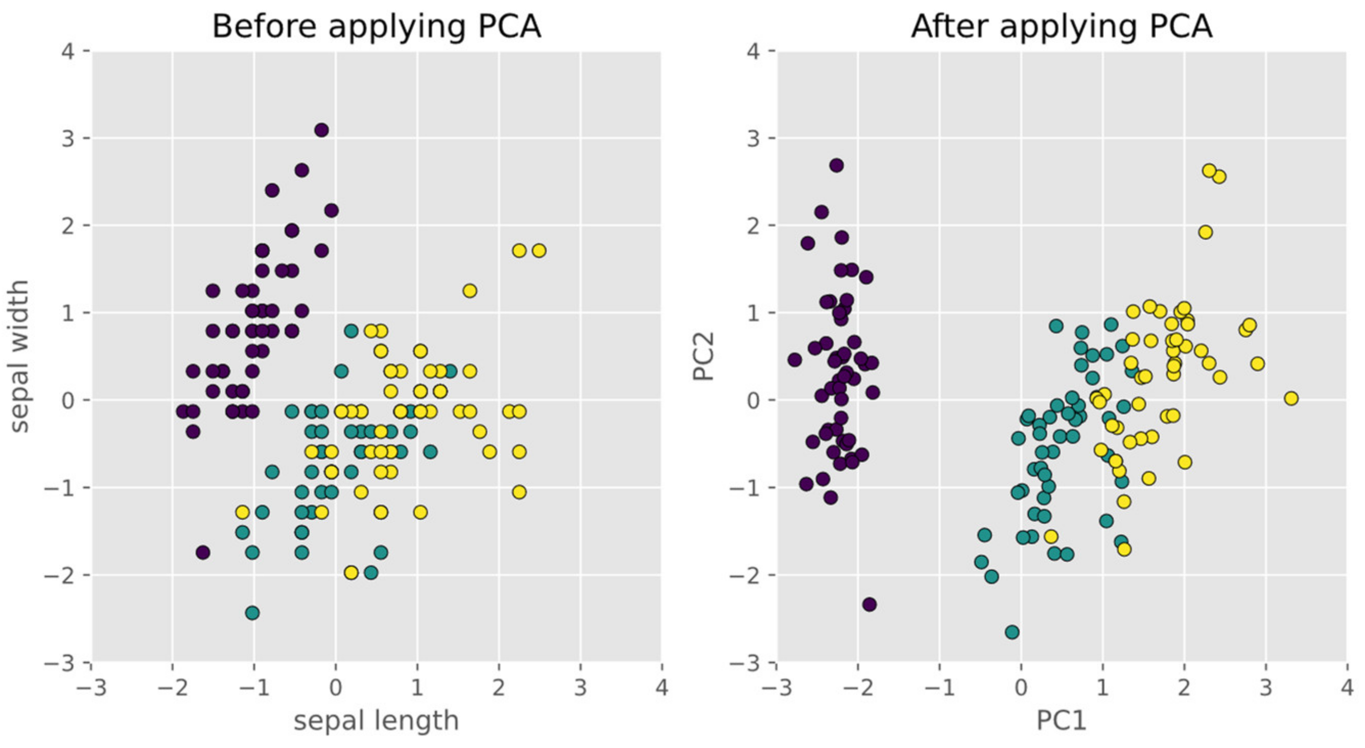
2. Principal Component Analysis (PCA)
3. EMOTHAW Databases
3.1. The DASS Scale
3.2. Subjects
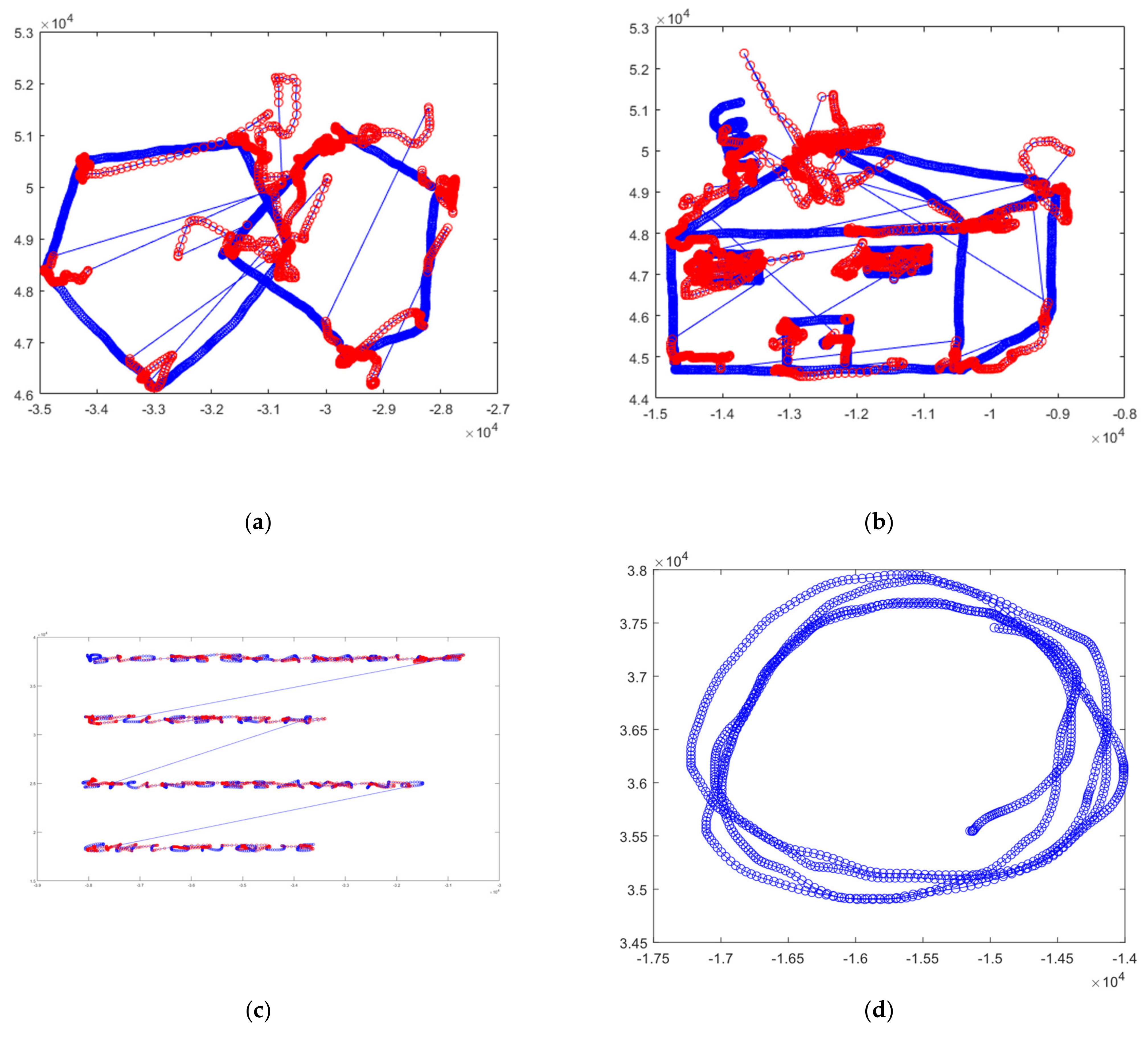
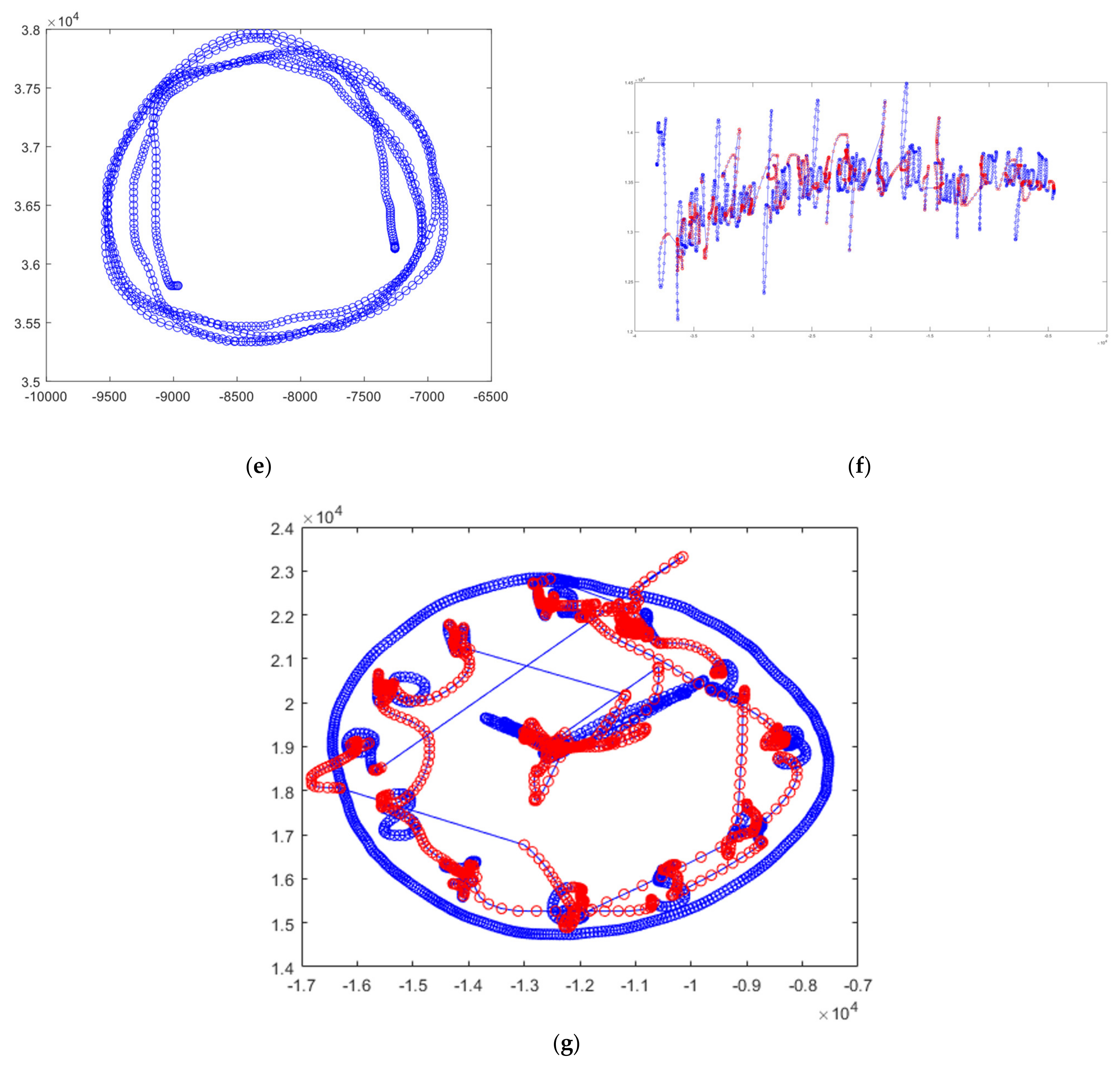
3.3. Tasks
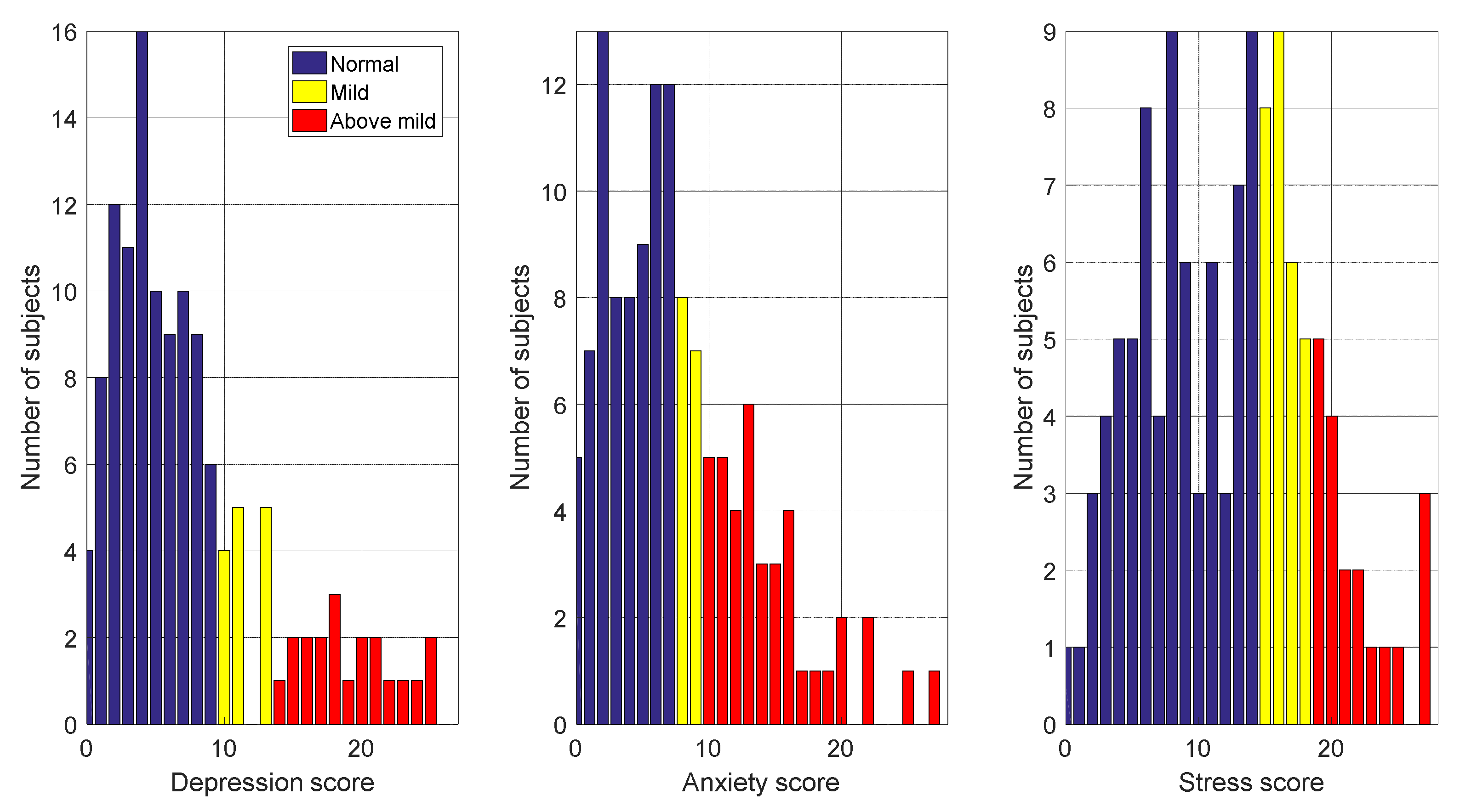
3.4. Distribution of Scores for Two and Three Mood States
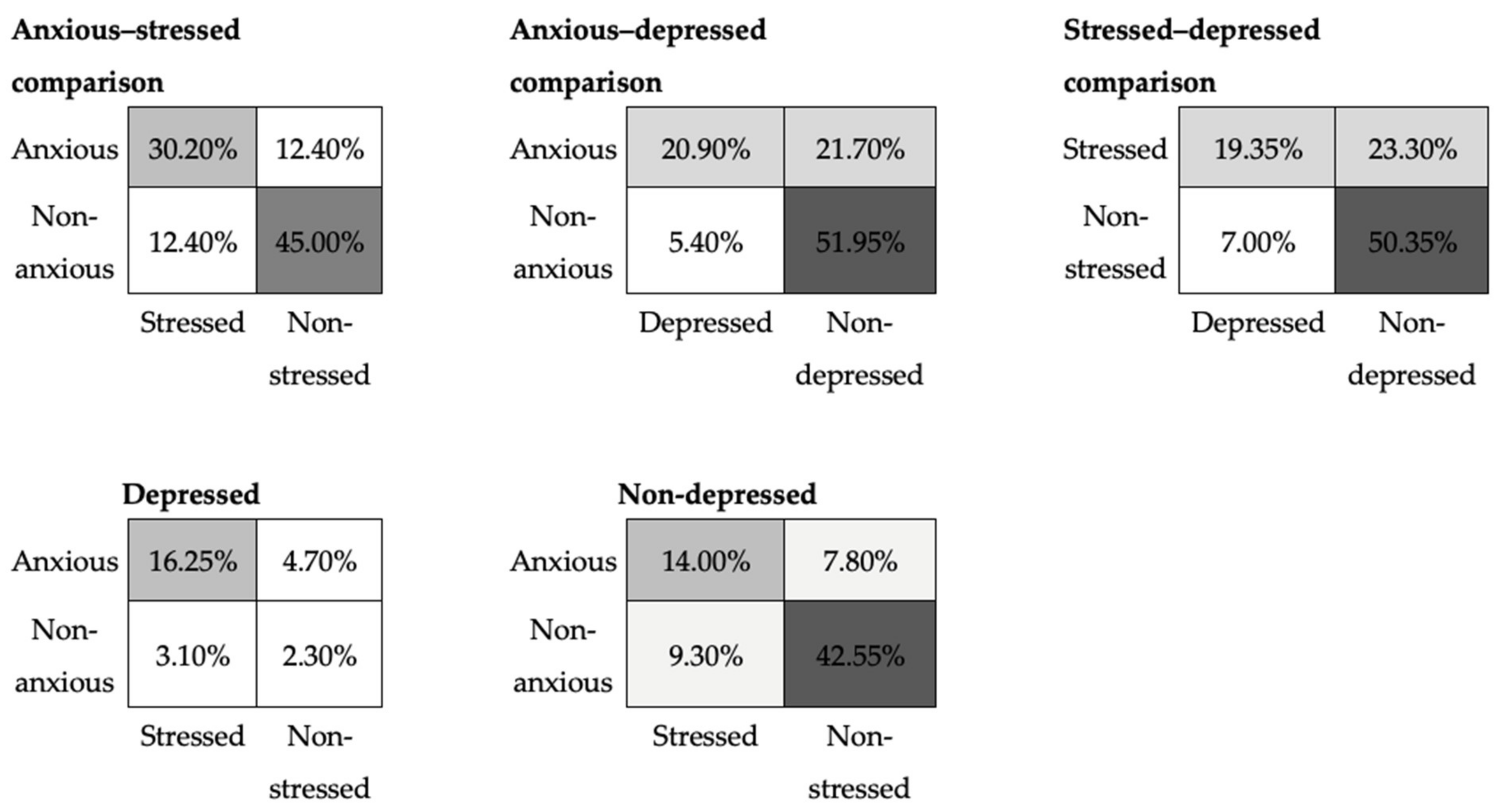
3.5. Overlapping of Mood States
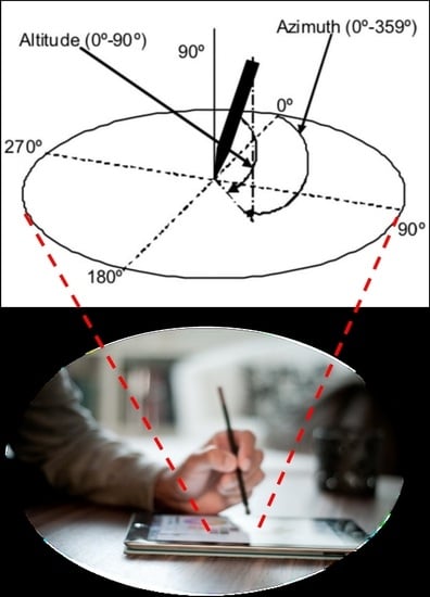
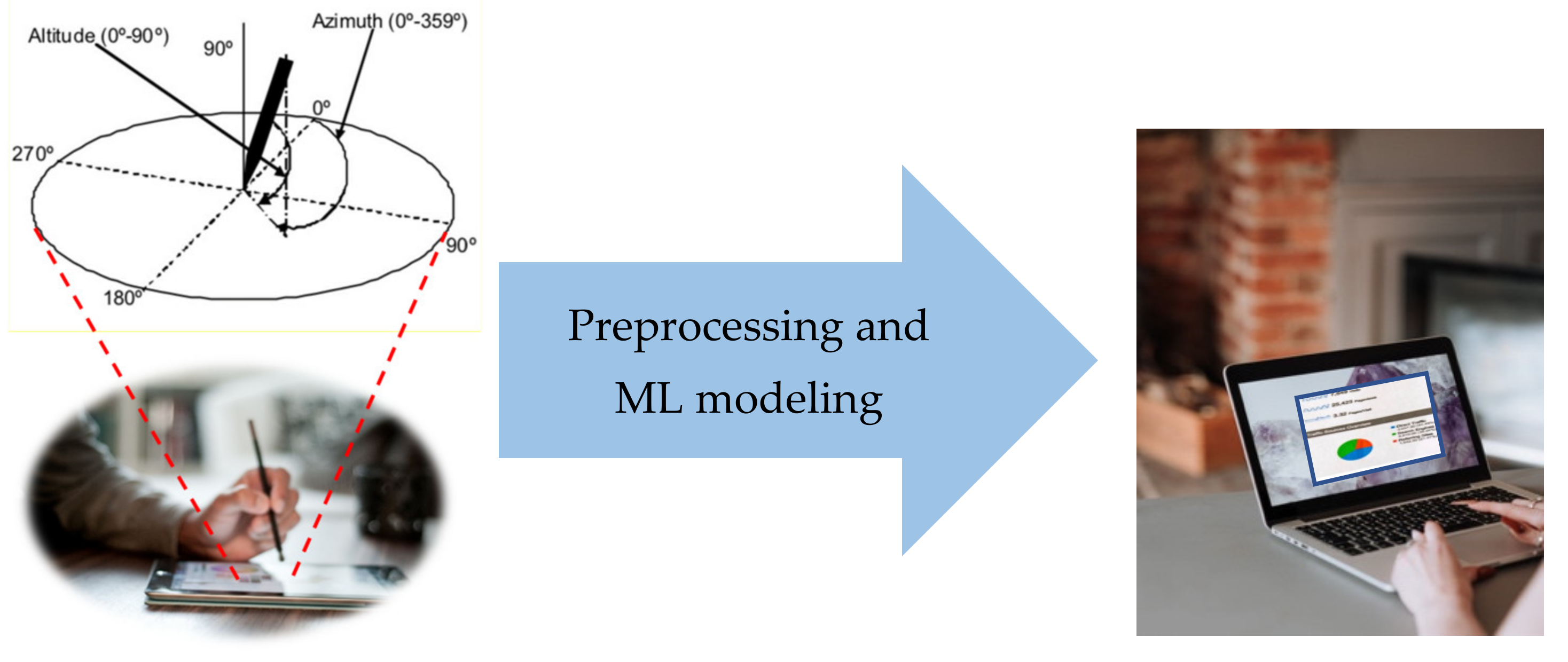
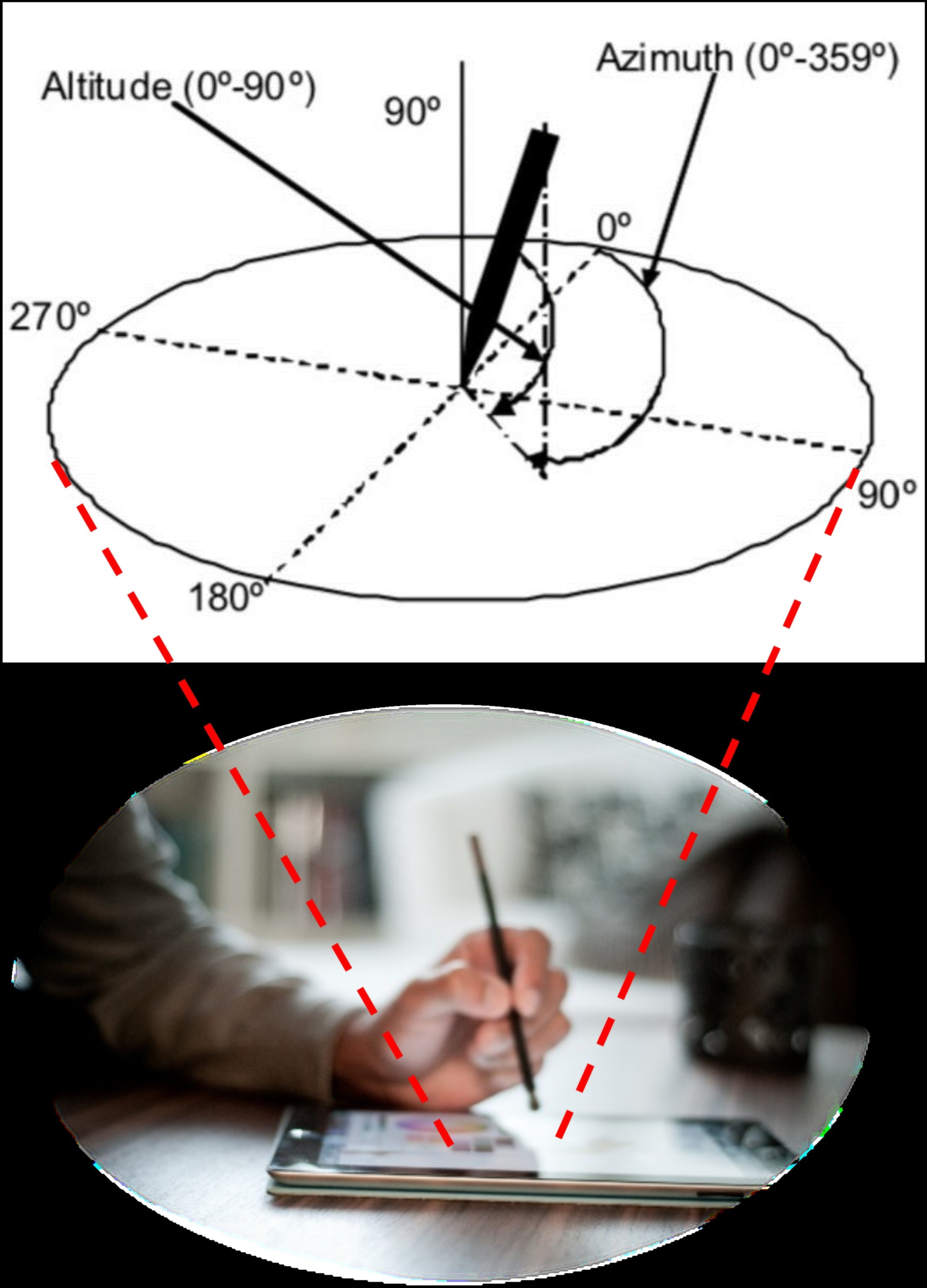
4. Sensors Data
- Horizontal position or displacement of the pen tip along the -axis, ;
- Vertical position or displacement of the pen tip along the -axis, ;
- Timestamps (in milliseconds), ;
- Pen status, that is, on-surface/in-air pen position status (touch/no-touch the paper),
- Altitude angle of the pen with respect to the tablet’s surface, ;
- Azimuth angle of the pen with respect to the tablet’s surface, ;
- Pressure applied by the pen tip on the tablet’s surface, .
Data Augmentation
- Identify the mood states having few observations,
- Calculate the number of samples required to make all the mood state observations of the same size,
- Randomly select observations from the original data and
- For each selected sample, calculate the new feature vector by adding the Gaussian random noise to the original features:
5. Feature Extraction
5.1. User’s Features
5.2. Detection Task
5.3. Features for Moods
6. Feature Selection
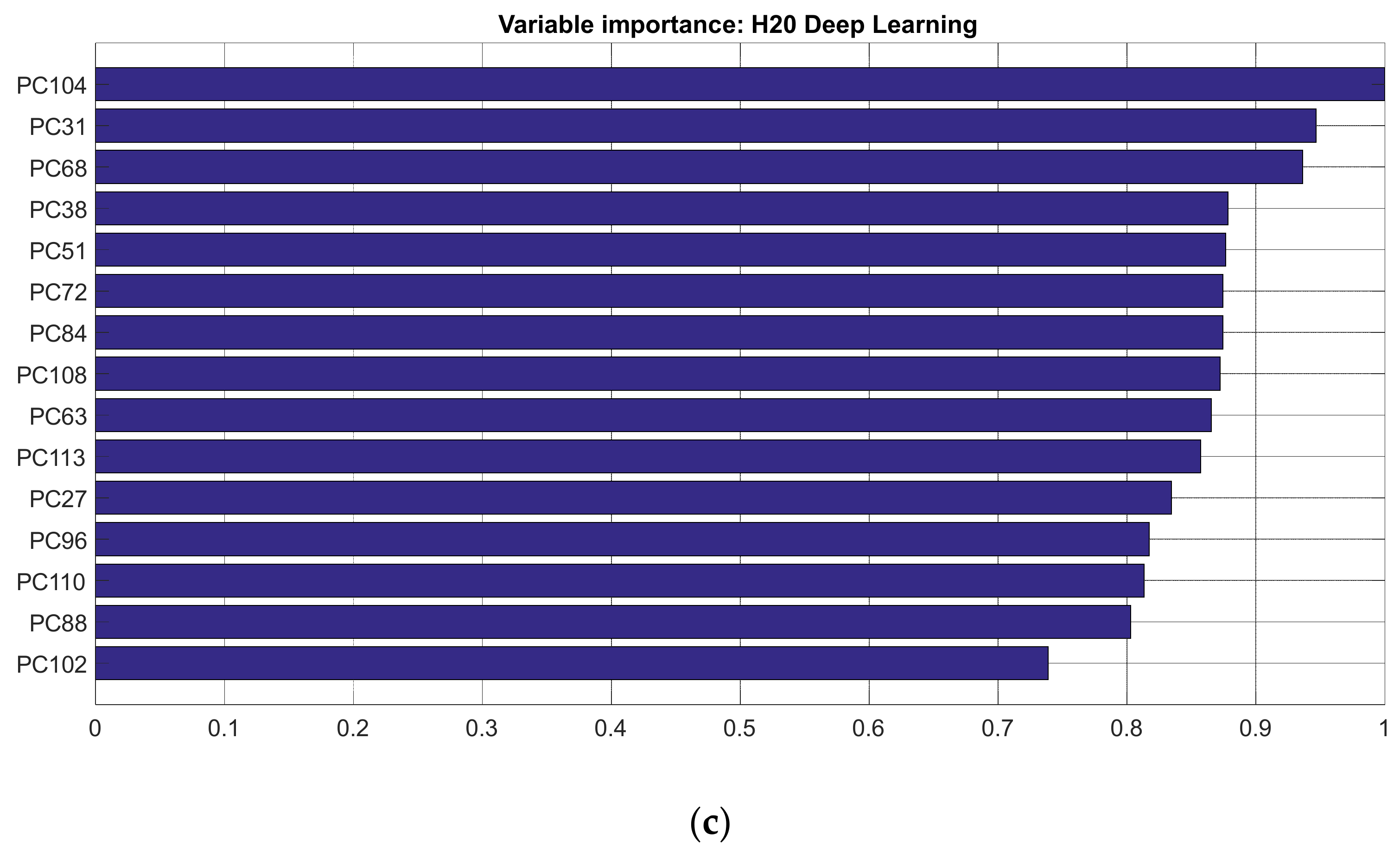
6.1. Principal Component Analysis (PCA)
6.2. Modified Fast Correlation-Based Filtering (mFCBF)
| Algorithm 1. The mFCBF algorithm receives the users’ feature matrix (), minimum correlation threshold () and the maximum correlation threshold () and returns the selected set of features. |
| 1: Function mFCBF (,, ) 2: Calculate corr () 3: Select columns whose correlation with the output is > 4: Calculate corr () 5: Select columns whose correlation with the input is < and with the highest correlation with the output. 6: Return () 7: End function |
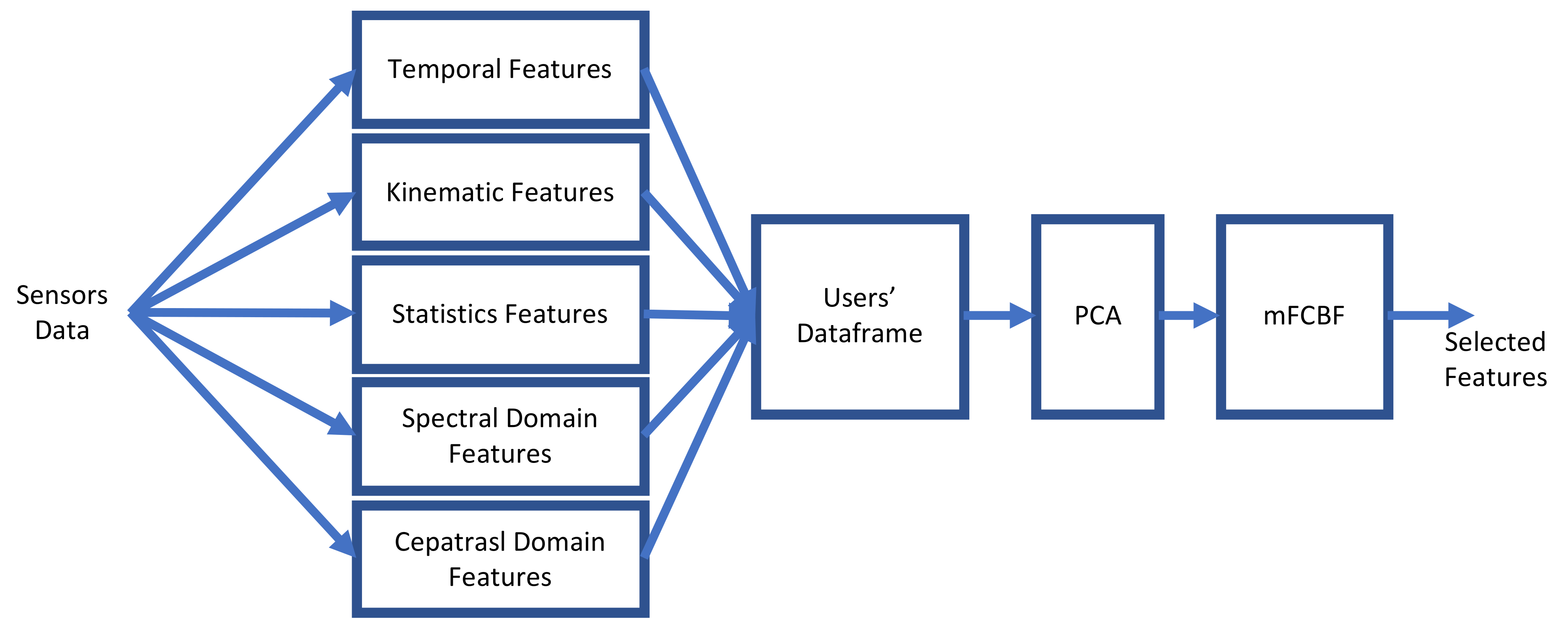
6.3. PCA-mFCBF Pipeline
7. Front-End Hyperparameters
8. ML Modelling to Maximise the Detection Task’s Accuracy
9. AutoML
AutoML H2O
10. Experiments and Results
11. Conclusions
Author Contributions
Funding
Institutional Review Board Statement
Informed Consent Statement
Data Availability Statement
Acknowledgments
Conflicts of Interest
References
- Plamondon, R.; Srihari, S. Online and off-line handwriting recognition: A comprehensive survey. IEEE Trans. Pattern Anal. Mach. Intell. 2000, 22, 63–84. [Google Scholar] [CrossRef] [Green Version]
- Li, S.Z.; Jain, A. Encyclopedia of Biometrics; Springer Publishing Company, Incorporated: New York, NY, USA, 2015. [Google Scholar]
- Faundez-Zanuy, M.; Fierrez, J.; Ferrer, M.A.; Diaz, M.; Tolosana, R.; Plamondon, R. Handwriting Biometrics: Applications and Future Trends in e-Security and e-Health. Cogn. Comput. 2020, 12, 940–953. [Google Scholar] [CrossRef]
- Stefano, C.D.; Fontanella, F.; Impedovo, D.; Pirlo, G.; Freca, A.S.D. Handwriting analysis to support neurodegenerative diseases diagnosis: A review. Pattern Recognit. Lett. 2019, 121, 37–45. [Google Scholar] [CrossRef]
- Depression and Other Common Mental Disorders, Global Health Estimates. Available online: https://apps.who.int/iris/bitstream/handle/10665/254610/WHO-MSD-MER-2017.2-eng.pdf (accessed on 14 December 2020).
- Scibelli, F.; Troncone, A.; Likforman-Sulem, L.; Vinciarelli, A.; Esposito, A. How Major Depressive Disorder Affects the Ability to Decode Multimodal Dynamic Emotional Stimuli. Front. ICT 2016, 3, 16. [Google Scholar] [CrossRef] [Green Version]
- Turner, A.I.; Smyth, N.; Hall, S.J.; Torres, S.J.; Hussein, M.; Jayasinghe, S.U.; Ball, K.; Clow, A.J. Psychological stress reactivity and future health and disease outcomes: A systematic review of prospective evidence. Psychoneuroendocrinology 2020, 114, 104599. [Google Scholar] [CrossRef] [PubMed]
- Esposito, A.; Raimo, G.; Maldonato, M.; Vogel, C.; Conson, M.; Cordasco, G. Behavioral Sentiment Analysis of Depressive States. In Proceedings of the 2020 11th IEEE International Conference on Cognitive Infocommunications (CogInfoCom), Mariehamn, Finland, 23–25 September 2020; pp. 209–214. [Google Scholar] [CrossRef]
- Beck, A.T.; Beamesderfer, A. Assessment of Depression: The Depression Inventory. Mod. Trends Pharm. Psychol. Meas. Psychopharmacol. 1974, 7, 151–169. [Google Scholar] [CrossRef]
- Schlenker, B.R.; Leary, M.R. Social anxiety and self-presentation: A conceptualization model. Psychol. Bull. 1982, 92, 641–669. [Google Scholar] [CrossRef] [PubMed]
- Spielberger, C.D. State-Trait Anxiety Inventory. In The Corsini Encyclopedia of Psychology, 4th ed.; John Wiley & Sons, Ltd.: Hoboken, NJ, USA, 2010. [Google Scholar] [CrossRef]
- Selye, H. The Stress of Life; McGraw-Hill: New York, NY, USA, 1984. [Google Scholar]
- Christensen, A.V.; Dixon, J.K.; Juel, K.; Ekholm, O.; Rasmussen, T.B.; Borregaard, B.; Mols, R.E.; Thrysøe, L.; Thorup, C.B.; Berg, S.K. Psychometric properties of the Danish Hospital Anxiety and Depression Scale in patients with cardiac disease: Results from the DenHeart survey. Health Qual. Life Outcomes 2020, 18, 1–13. [Google Scholar] [CrossRef] [PubMed]
- Tolosana, R.; Vera-Rodriguez, R.; Fierrez, J.; Morales, A.; Ortega-Garcia, J. Benchmarking desktop and mobile handwriting across COTS devices: The e-BioSign biometric database. PLoS ONE 2017, 12, e0176792. [Google Scholar] [CrossRef] [PubMed]
- Likforman-Sulem, L.; Esposito, A.; Faundez-Zanuy, M.; Clemencon, S.; Cordasco, G. EMOTHAW: A Novel Database for Emotional State Recognition from Handwriting and Drawing. IEEE Trans. Hum.-Mach. Syst. 2017, 47, 273–284. [Google Scholar] [CrossRef]
- Nolazco-Flores, J.A.; Faundez-Zanuy, M.; Velázquez-Flores, O.A.; Cordasco, G.; Esposito, A. Emotional State Recognition Performance Improvement on a Handwriting and Drawing Task. IEEE Access 2021, 9, 28496–28504. [Google Scholar] [CrossRef]
- Nolazco-Flores, J.A.; Faundez-Zanuy, M.; de la Cueva, V.M.; Mekyska, J. Exploiting Spectral and Cepstral Handwriting Features on Diagnosing Parkinson’s Disease. IEEE Access 2021, 9, 141599–141610. [Google Scholar] [CrossRef]
- Yu, L.; Liu, H. Feature selection for high-dimensional data: A fast correlation-based filter solution. In Proceedings of the 20th International Conference on Machine Learning (ICML-03), Washington, DC, USA, 21–24 August 2003; pp. 856–863. [Google Scholar]
- Rabus, D.G.; Rebener, K.; Sada, C. Optofluidics: Process Analytical Technology; Walter de Gruyter: Berlin, Germany, 2018; pp. vii–viii. [Google Scholar] [CrossRef]
- Guiot, J.; de Vernal, A. Chapter Thirteen Transfer Functions: Methods for Quantitative Paleoceanography Based on Microfossils. In Developments in Marine Geology; Hillaire–Marcel, C., de Vernal, A., Eds.; Elsevier: Amsterdam, The Netherlands, 2007; Volume 1, pp. 523–563. [Google Scholar] [CrossRef]
- Cochi, M.; Vigni, M.L.; Durante, C. Chemometrics—Bioinformatics. In Food Authentication: Management, Analysis and Regulation; Gerogious, C.A., Danezis, G.P., Eds.; John Wiley & Sons, Ltd.: Hoboken, NJ, USA, 2017; pp. 481–518. [Google Scholar] [CrossRef]
- Horn, R.A.; Johnson, C.R. Matrix Analysis; Cambridge University Press: Cambridge, UK, 1985; ISBN 978-0-521-38632-6. [Google Scholar]
- The Iris Dataset. Available online: https://scikit-learn.org/stable/auto_examples/datasets/plot_iris_dataset.html (accessed on 31 October 2021).
- Folstein, M.F.; Folstein, S.E.; Mchugh, P.R. Mini-mental state. J. Psychiatr. Res. 1975, 12, 189–198. [Google Scholar] [CrossRef]
- Kline, P. Handbook of Psychological Testing; Routlege: Abingdon-on-Thames, UK, 2013. [Google Scholar]
- Depression Anxiety Stress Scales (DASS). Available online: https://www.psytoolkit.org/survey-library/depression-anxiety-stress-dass.html (accessed on 10 November 2021).
- Severino Italian Translation. Available online: http://www2.psy.unsw.edu.au/dass/Italian/Severino.htm (accessed on 13 December 2020).
- H2O AutoML. Available online: https://www.h2o.ai/products/h2o-automl (accessed on 31 October 2021).
- The H2O Python Module. Available online: https://docs.h2o.ai/h2o/latest-stable/h2o-py/docs/intro.html (accessed on 30 November 2021).
- PyCaret. Available online: https://pycaret.org (accessed on 30 November 2021).
- PyCaret 2.3.6 is Here! Learn What’s New? Available online: https://towardsdatascience.com/pycaret-2-3-6-is-here-learn-whats-new-1479c8bab8ad (accessed on 2 January 2022).
- auto-sklearn. Available online: https://automl.github.io/auto-sklearn/master (accessed on 30 November 2021).
- Feurer, M.; Klein, A.; Eggensperger, K.; Springenberg, J.; Blum, M.; Hutter, F. Efficient and robust automated machine learning. In Advances in Neural Information Processing Systems 28; Cortes, C., Lawrence, N.D., Lee, D.D., Sugiyama, M., Garnett, R., Eds.; MIT Press: Cambridge, Massachusetts, USA, 2015; pp. 2962–2970. [Google Scholar]
- Le, T.T.; Fu, W.; Moore, J.H. Scaling tree-based automated machine learning to biomedical big data with a feature set selector. Bioinformatics 2020, 36, 250–256. [Google Scholar] [CrossRef] [PubMed] [Green Version]
- Olson, R.S.; Bartley, N.; Urbanowicz, R.J.; Moore, J.H. Evaluation of a tree-based pipeline optimization tool for automating data science. In Proceedings of the Genetic and Evolutionary Computation Conference 2016, GECCO’16, Denver, CO, USA, 20–24 July 2016; ACM: New York, NY, USA, 2016; pp. 485–492. [Google Scholar] [CrossRef] [Green Version]
- Olson, R.S.; Urbanowicz, R.J.; Andrews, P.C.; Lavender, N.A.; Kidd, L.C.; Moore, J.H. Automating Biomedical Data Science through Tree-Based Pipeline Optimization. In Applications of Evolutionary Computation, Proceedings of 19th European Conference, EvoApplications 2016, Porto, Portugal, 30 March–1 April 2016; Squillero, G., Burelli, P., Eds.; Springer: Cham, Switzerland; pp. 123–137. [CrossRef] [Green Version]
- MLBox, Machine Learning Box. Available online: https://mlbox.readthedocs.io/en/latest (accessed on 30 November 2021).
- SciKit-Learn, Machine Learning in Python. Available online: https://scikit-learn.org/stable (accessed on 30 November 2021).


| Binary Labeling Used in [15] | Trinary Labeling | Interpretation of DASS | Depression | Anxiety | Stress |
|---|---|---|---|---|---|
| Normal | Normal | Normal | 0–9 | 0–7 | 0–14 |
| Above normal | Mild | Mild | 10–13 | 8–9 | 15–18 |
| Above mild | Moderate | 14–20 | 10–14 | 19–25 | |
| Severe | 21–27 | 15–19 | 26–33 | ||
| Extremely severe | 28+ | 20+ | 34+ |
| Tasks |
|---|
|
|
|
|
|
|
|
| Notation | Definition |
|---|---|
| Pen’s displacement at the sample | |
| Trajectory taken during handwriting divided by the duration of writing | |
| On-air pen duration | |
| On-paper pen duration | |
| Duration of the stroke | |
| normalised to writing duration | |
| Ratio of time the pen spent in air or on the tablet’s surface | |
| Number of changes in the direction of the velocity vector | |
| Number of changes in direction of the acceleration vector | |
| relative to writing duration | |
| relative to writing duration |
| Notation | Definition |
|---|---|
| Notation | Definition | |
|---|---|---|
(basic statistics features) | ||
(mean features) | ||
(momentum features) | ||
| Classification Algorithms |
|---|
| Deep neural network (DNN) |
| Distributed random forest (DRF) |
| Extremely randomised trees (ERT) |
| Generalised linear model (GLM) |
| Gradient boosting machine (GBM) |
| Naïve Bayes classifier (NBC) |
| Rulefit (RF) |
| Stacked ensembles (SE) |
| XGBoost (XGB) |
| Support vector machine (SVM) |
| Parameter | Value |
|---|---|
| max_runtime_secs | 200 |
| max_models | 15 |
| exclude_algos | GBM |
| seed | 1 |
| nfolds | 2 |
| stopping_metric | logloss |
| [16] | ||
|---|---|---|
| Depression | 71.47 | 80.70 |
| Anxiety | 58.53 | 71.93 |
| Stress | 61.24 | 66.67 |
| [16] | ||||||
|---|---|---|---|---|---|---|
| Depression | 74.01 | 79.82 | 74.01 | 88.60 | 87.40 | 92.10 |
| Anxiety | 62.20 | 71.05 | 72.44 | 81.58 | 83.46 | 85.96 |
| Stress | 57.48 | 68.42 | 70.07 | 81.58 | 85.03 | 88.59 |
| Depression | 79.82 | 81.57 | 88.60 | 92.98 | 92.10 | 100.00 |
| Anxiety | 71.05 | 75.43 | 81.58 | 88.60 | 85.96 | 100.00 |
| Stress | 68.42 | 71.92 | 81.58 | 89.47 | 88.59 | 100.00 |
| Depression | 74.56 | 77.19 | 81.57 | 82.45 |
| Anxiety | 50.87 | 57.89 | 71.92 | 72.80 |
| Stress | 47.36 | 54.38 | 65.78 | 74.56 |
Publisher’s Note: MDPI stays neutral with regard to jurisdictional claims in published maps and institutional affiliations. |
© 2022 by the authors. Licensee MDPI, Basel, Switzerland. This article is an open access article distributed under the terms and conditions of the Creative Commons Attribution (CC BY) license (https://creativecommons.org/licenses/by/4.0/).
Share and Cite
Nolazco-Flores, J.A.; Faundez-Zanuy, M.; Velázquez-Flores, O.A.; Del-Valle-Soto, C.; Cordasco, G.; Esposito, A. Mood State Detection in Handwritten Tasks Using PCA–mFCBF and Automated Machine Learning. Sensors 2022, 22, 1686. https://doi.org/10.3390/s22041686
Nolazco-Flores JA, Faundez-Zanuy M, Velázquez-Flores OA, Del-Valle-Soto C, Cordasco G, Esposito A. Mood State Detection in Handwritten Tasks Using PCA–mFCBF and Automated Machine Learning. Sensors. 2022; 22(4):1686. https://doi.org/10.3390/s22041686
Chicago/Turabian StyleNolazco-Flores, Juan Arturo, Marcos Faundez-Zanuy, Oliver Alejandro Velázquez-Flores, Carolina Del-Valle-Soto, Gennaro Cordasco, and Anna Esposito. 2022. "Mood State Detection in Handwritten Tasks Using PCA–mFCBF and Automated Machine Learning" Sensors 22, no. 4: 1686. https://doi.org/10.3390/s22041686
APA StyleNolazco-Flores, J. A., Faundez-Zanuy, M., Velázquez-Flores, O. A., Del-Valle-Soto, C., Cordasco, G., & Esposito, A. (2022). Mood State Detection in Handwritten Tasks Using PCA–mFCBF and Automated Machine Learning. Sensors, 22(4), 1686. https://doi.org/10.3390/s22041686