
Smooth Complete Coverage Trajectory Planning Algorithm for a Nonholonomic Robot


Abstract
1. Introduction
2. Related Work
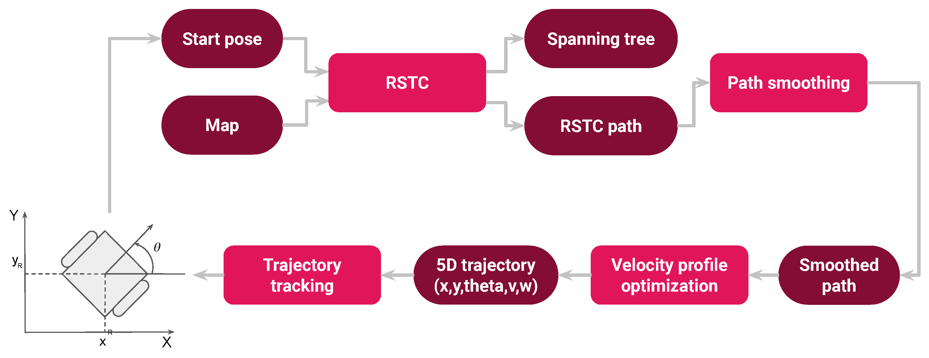
3. The Proposed Smooth Complete Coverage Path Planning Algorithm
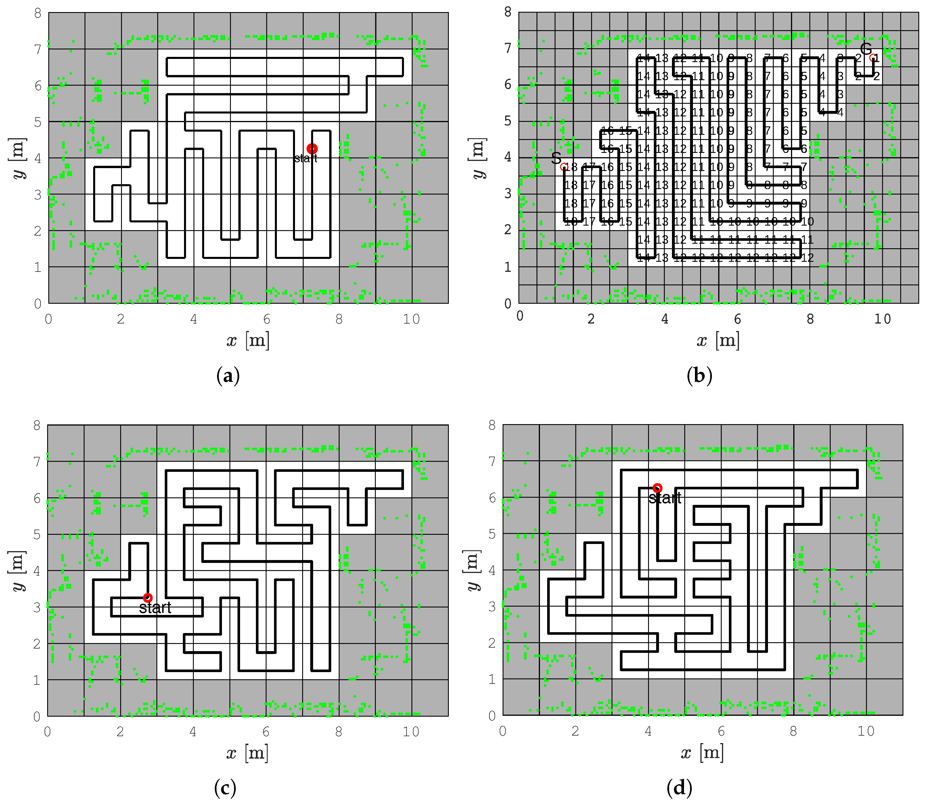
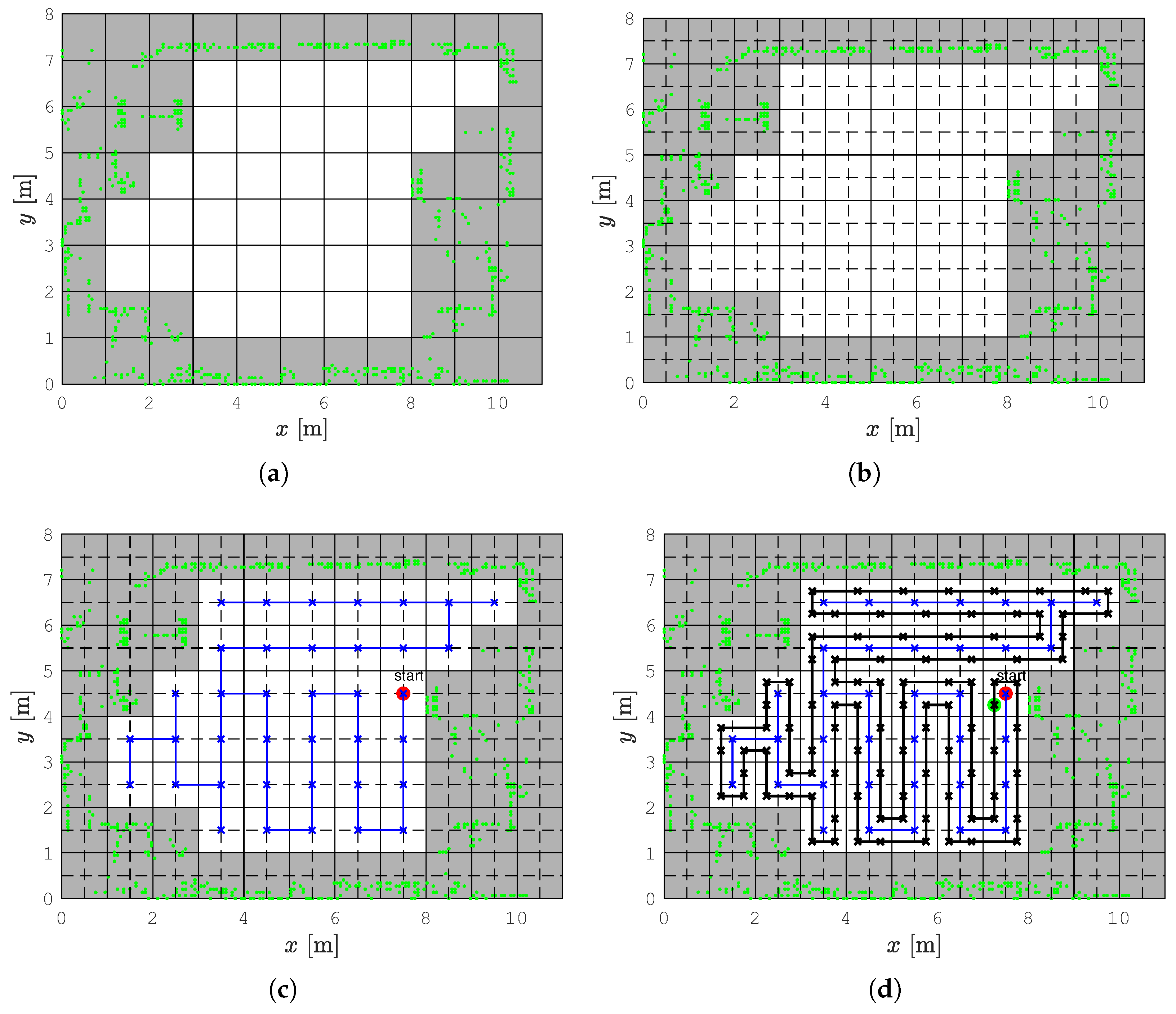
3.1. The Replanning Spanning Tree Coverage Algorithm
| Algorithm 1 Pseudocode for the spanning tree |
|
| Algorithm 2 Pseudocode for the path planning |
|
| Algorithm 3 Pseudocode for the complete coverage path planning |
|
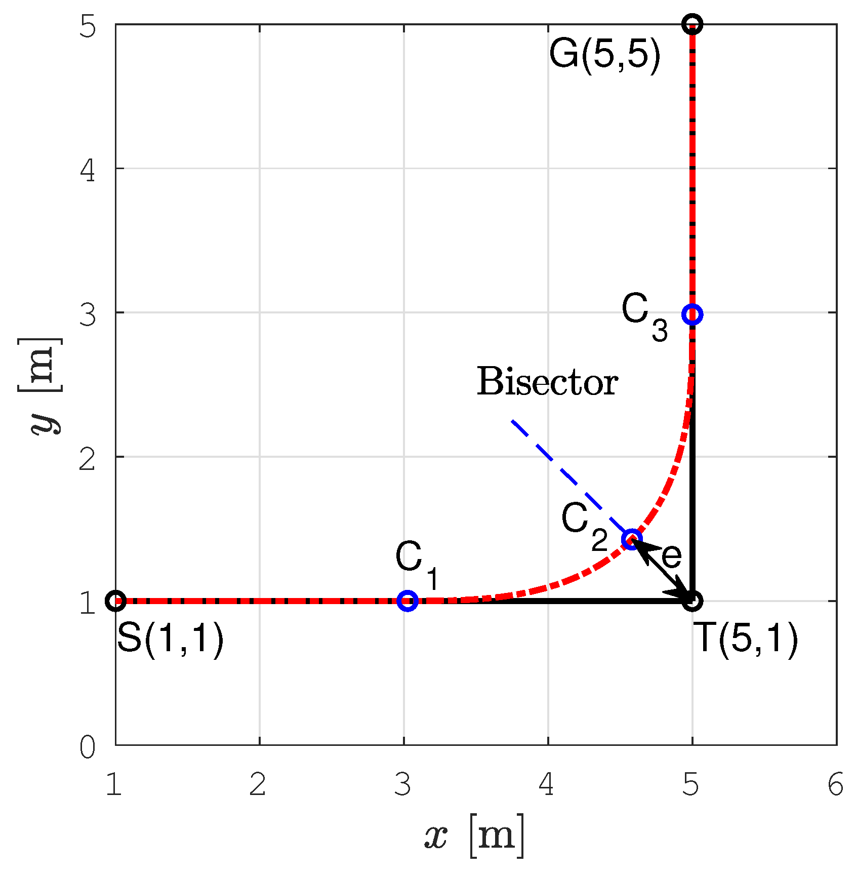
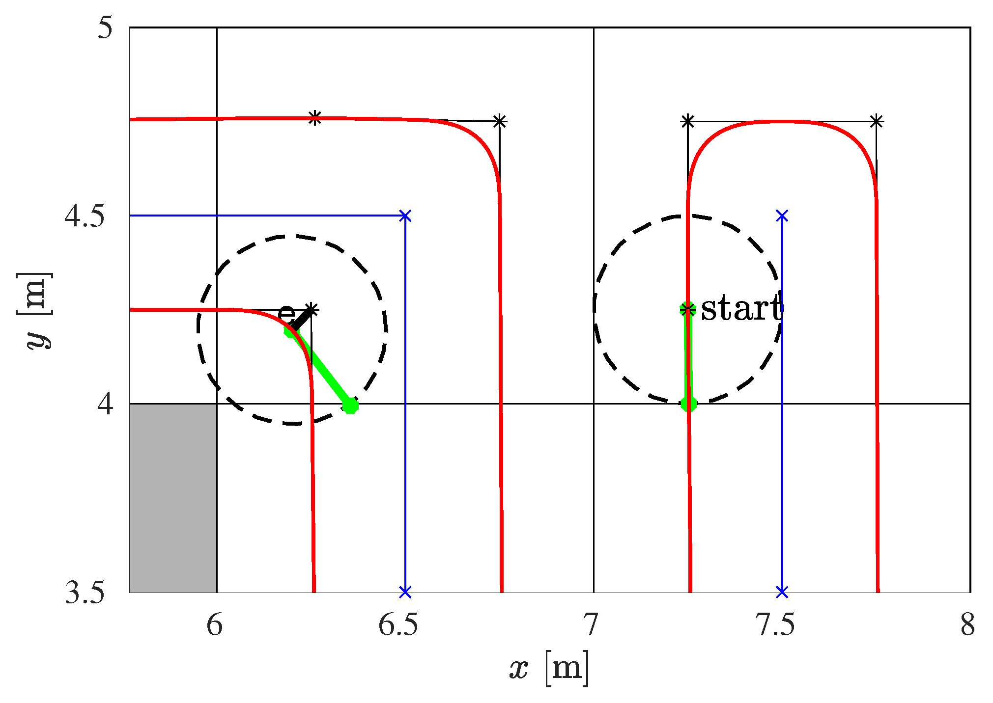
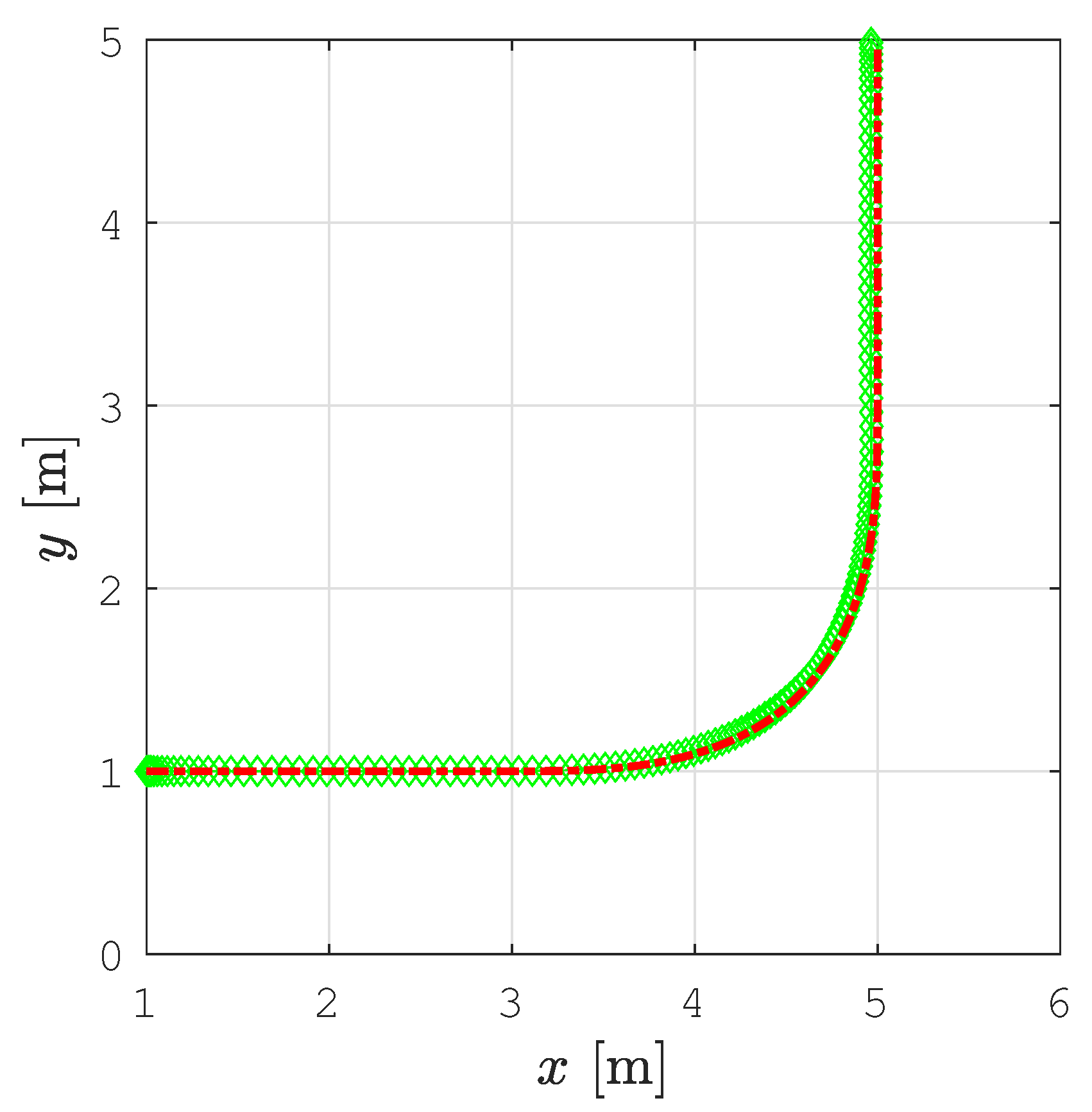
3.2. Path Smoothing
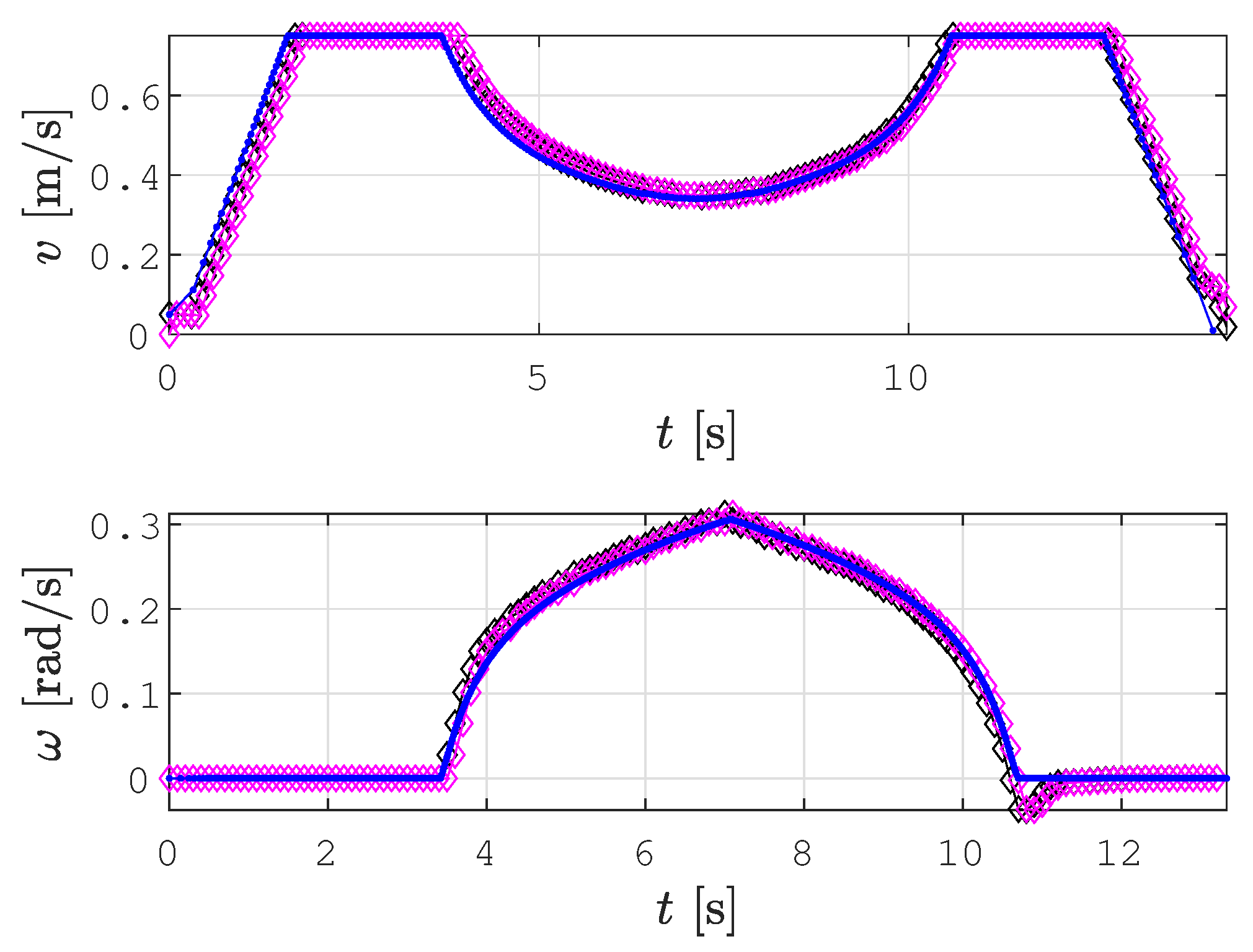
3.3. Velocity Profile Optimization and Trajectory Tracking
4. Simulation Results
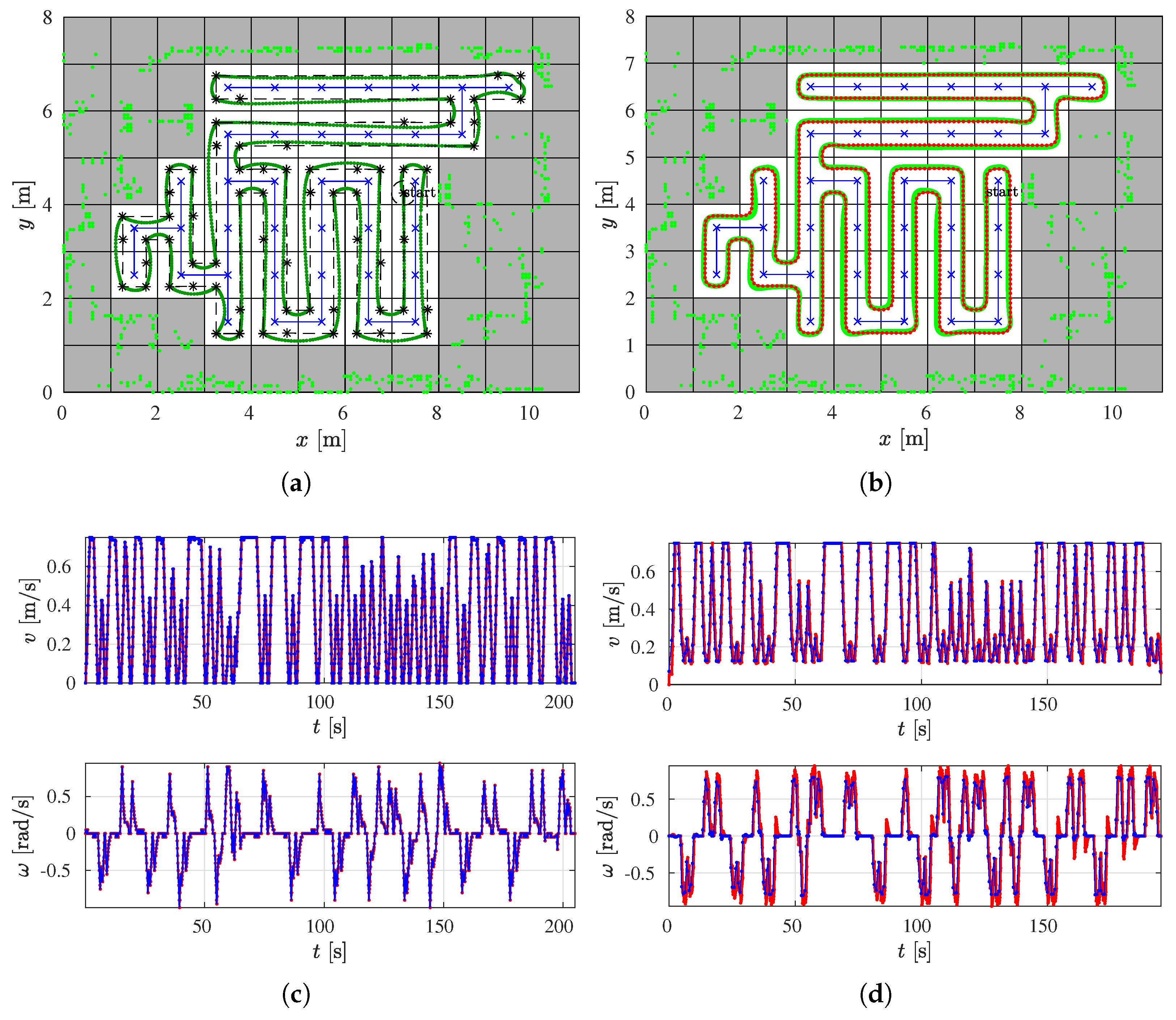
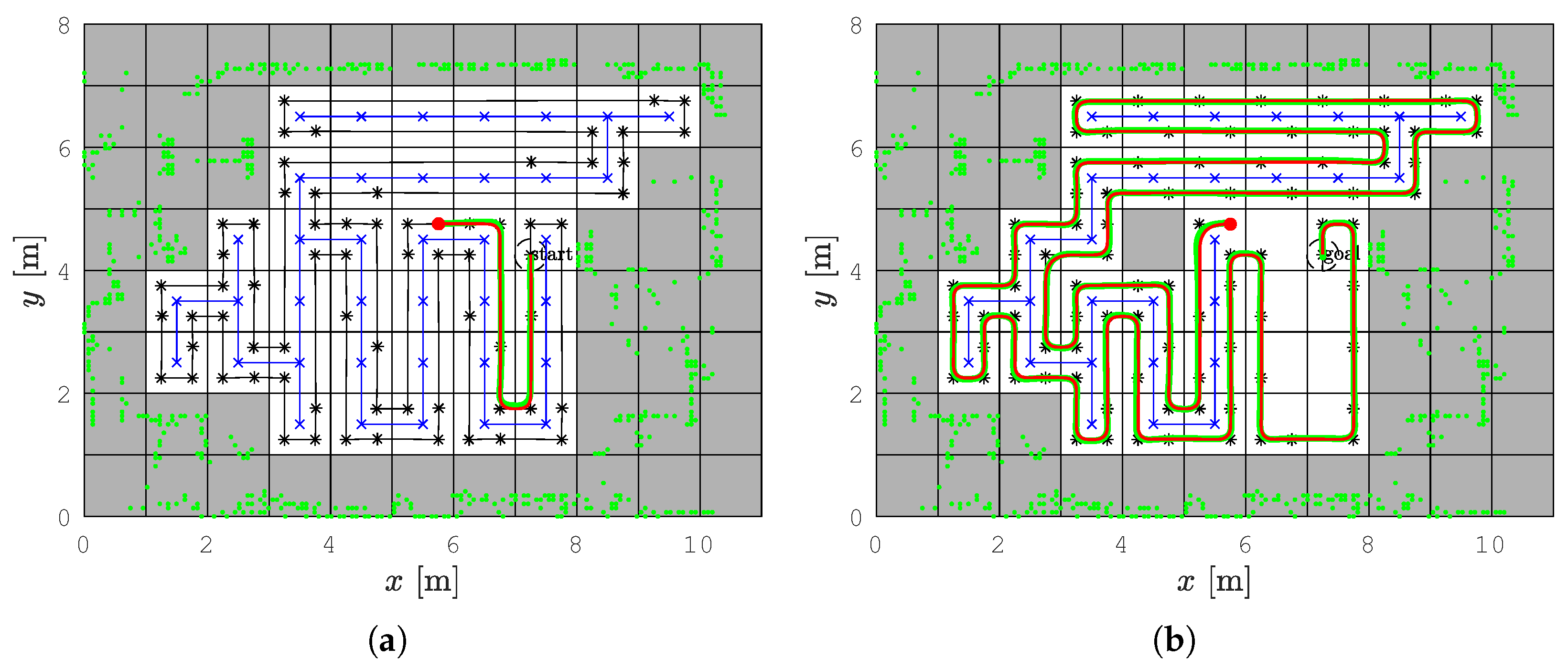
4.1. The Lab Scenario
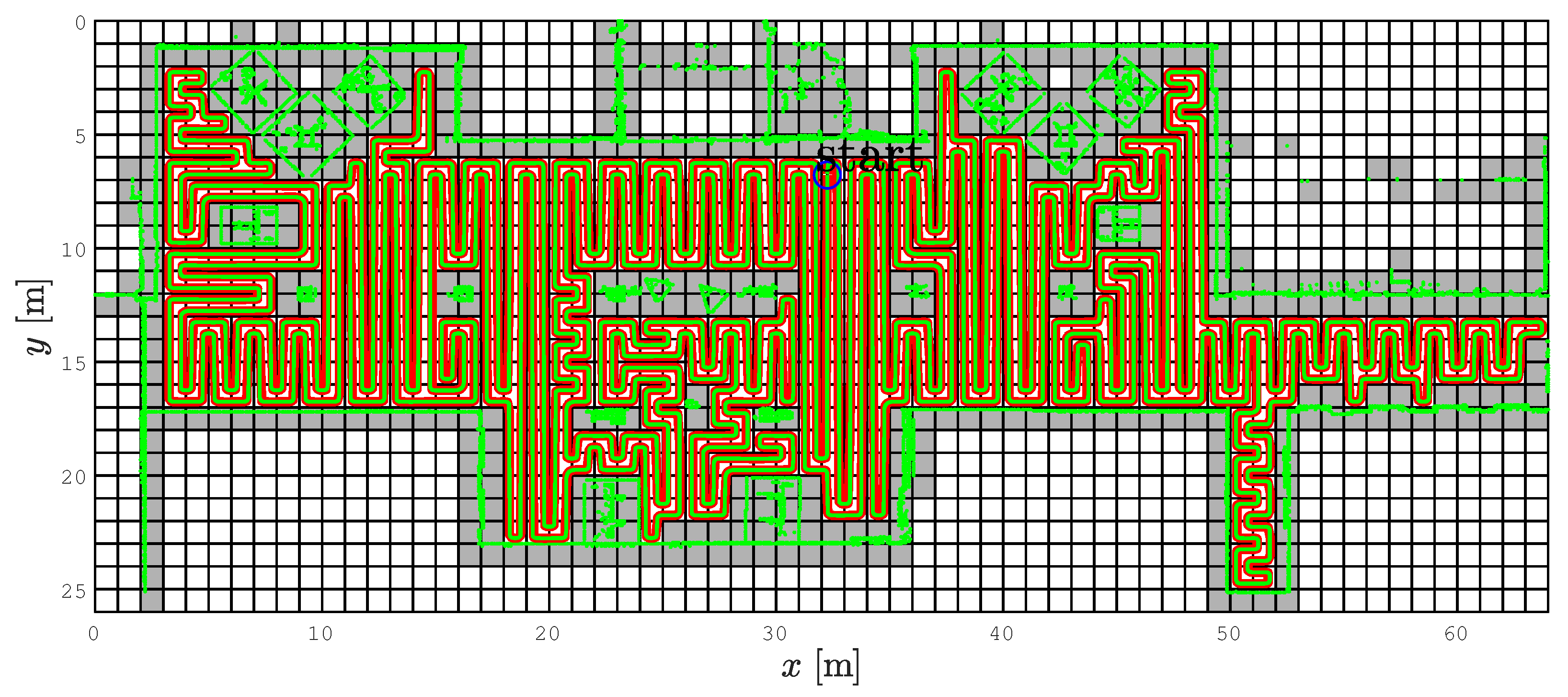
4.2. The Aula Scenario
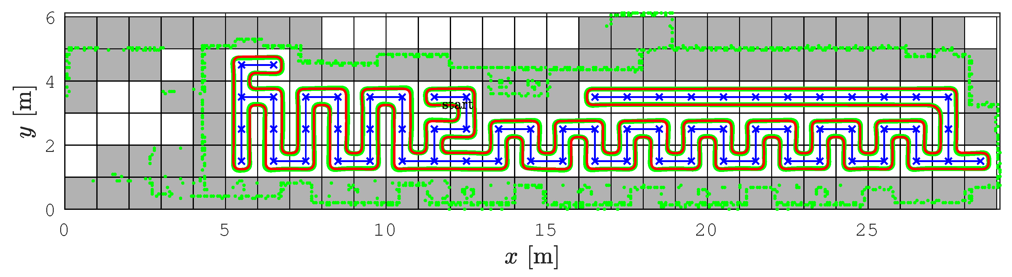
4.3. The Gallery Scenario
4.4. Discussion
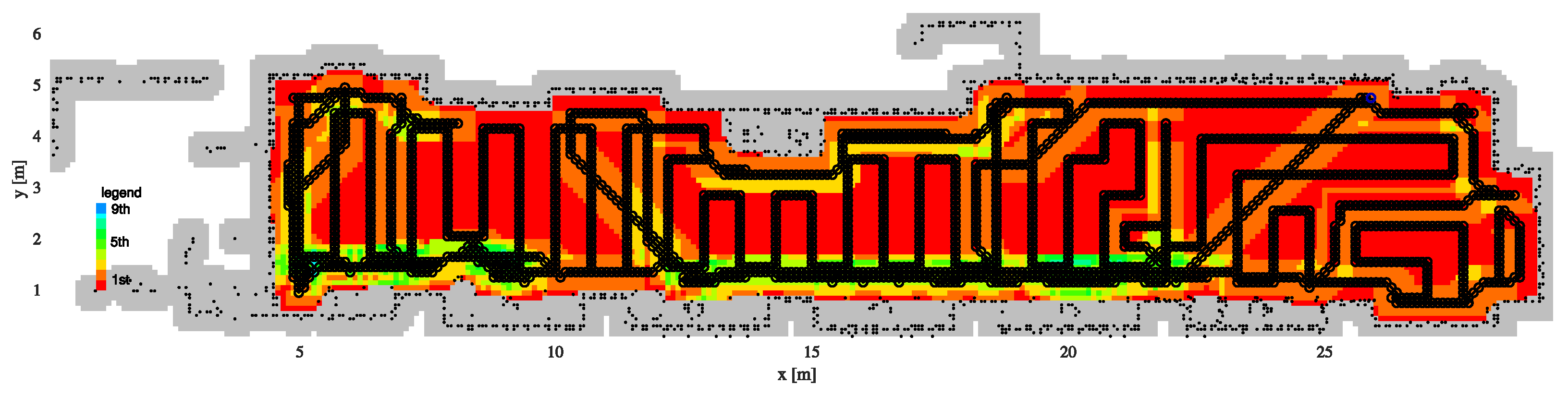
5. Experiments on a Real Robot
6. Conclusions
Author Contributions
Funding
Institutional Review Board Statement
Informed Consent Statement
Data Availability Statement
Conflicts of Interest
References
- Gao, X.S.; Xu, D.G.; Wang, Y. Omni-directional mobile robot for floor cleaning. Chin. J. Mech. Eng. 2008, 44, 228–233. [Google Scholar] [CrossRef]
- Dakulović, M.; Horvatić, S.; Petrović, I. Complete Coverage D* Algorithm for Path Planning of a Floor-Cleaning Mobile Robot. In Proceedings of the Preprints of the 18th IFAC World Congress, Milano, Italy, 28 August–2 September 2011; pp. 5950–5955. [Google Scholar] [CrossRef]
- Yang, S.X.; Luo, C. A neural network approach to complete coverage path planning. IEEE Trans. Syst. Man Cybern. Part B (Cybern.) 2004, 34, 718–724. [Google Scholar] [CrossRef] [PubMed]
- Acar, E.; Choset, H.; Zhang, Y.; Schervish, M. Path Planning for Robotic Demining: Robust Sensor-Based Coverage of Unstructured Environments and Probabilistic Methods. Int. J. Robot. Res. 2003, 22, 441–466. [Google Scholar] [CrossRef]
- Dakulović, M.; Petrović, I. Complete coverage path planning of mobile robots for humanitarian demining. Ind. Robot. Int. J. 2012, 39, 484–493. [Google Scholar] [CrossRef]
- Ollis, M.; Stentz, A. First results in vision-based crop line tracking. In Proceedings of the IEEE International Conference on Robotics and Automation, Minneapolis, MN, USA, 22–28 April 1996; pp. 951–956. [Google Scholar] [CrossRef]
- Weiss-Cohen, M.; Sirotin, I.; Rave, E. Lawn Mowing System for Known Areas. In Proceedings of the 2008 International Conference on Computational Intelligence for Modelling Control & Automation, Vienna, Austria, 10–12 December 2008; pp. 539–544. [Google Scholar] [CrossRef]
- Kapoutsis, A.C.; Chatzichristofis, S.A.; Doitsidis, L.; de Sousa, J.B.; Kosmatopoulos, E.B. Autonomous navigation of teams of Unmanned Aerial or Underwater Vehicles for exploration of unknown static dynamic environments. In Proceedings of the 21st Mediterranean Conference on Control and Automation, Platanias, Greece, 25–28 June 2013; pp. 1181–1188. [Google Scholar] [CrossRef]
- Kapoutsis, A.; Chatzichristofis, S.; Doitsidis, L.; Sousa, J.; Pinto, J.; Braga, J.; Kosmatopoulos, E. Real-time adaptive multi-robot exploration with application to underwater map construction. Auton. Robot. 2015, 40, 987–1015. [Google Scholar] [CrossRef]
- Šelek, A.; Seder, M.; Petrović, I. Mobile robot navigation for complete coverage of an environment. IFAC-PapersOnLine 2018, 51, 512–517. [Google Scholar] [CrossRef]
- Brezak, M.; Petrović, I. Path smoothing using clothoids for differential drive mobile robots. IFAC Proc. Vol. 2011, 44, 1133–1138. [Google Scholar] [CrossRef]
- Cao, Z.L.; Huang, Y.; Hall, E.L. Region filling operations with random obstacle avoidance for mobile robotics. J. Robot. Syst. 1988, 5, 87–102. [Google Scholar] [CrossRef]
- Galceran, E.; Carreras, M. A Survey on Coverage Path Planning for Robotics. Robot. Auton. Syst. 2013, 61, 1258–1276. [Google Scholar] [CrossRef]
- An, V.; Qu, Z.; Roberts, R. A Rainbow Coverage Path Planning for a Patrolling Mobile Robot With Circular Sensing Range. IEEE Trans. Syst. Man Cybern. Syst. 2017, 48, 1238–1254. [Google Scholar] [CrossRef]
- An, V.; Qu, Z.; Crosby, F.; Roberts, R.; An, V. A Triangulation-Based Coverage Path Planning. IEEE Trans. Syst. Man Cybern. Syst. 2020, 50, 2157–2169. [Google Scholar] [CrossRef]
- Zelinsky, A.; Jarvis, R.; Byrne, J.C.; Yuta, S. Planning Paths of Complete Coverage of an Unstructured Environment by a Mobile Robot. In Proceedings of the International Conference on Advanced Robotics, Tokyo, Japan, 26–30 July 1993; pp. 533–538. [Google Scholar]
- Gabriely, Y.; Rimon, E. Competitive online coverage of grid environments by a mobile robot. Comput. Geom. 2003, 24, 197–224. [Google Scholar] [CrossRef]
- Dakulović, M.; Čikeš, M.; Petrović, I. Efficient Interpolated Path Planning of Mobile Robots based on Occupancy Grid Maps. IFAC Proc. Vol. 2012, 45, 349–354. [Google Scholar] [CrossRef]
- Klančar, G.; Seder, M.; Blažič, S.; Škrjanc, I.; Petrović, I. Drivable Path Planning Using Hybrid Search Algorithm Based on E* and Bernstein-Bézier Motion Primitives. IEEE Trans. Syst. Man Cybern. Syst. 2019, 51, 4868–4882. [Google Scholar] [CrossRef]
- Le, A.V.; Prabakaran, V.; Sivanantham, V.; Mohan, R.E. Modified A-Star Algorithm for Efficient Coverage Path Planning in Tetris Inspired Self-Reconfigurable Robot with Integrated Laser Sensor. Sensors 2018, 18, 2585. [Google Scholar] [CrossRef] [PubMed]
- Lui, Y.T.; Sun, R.Z.; Zhang, T.Y.; Zhang, X.N.; Li, L.; Shi, G.Q. Warehouse-Oriented Optimal Path Planning for Autonomous Mobile Fire-Fighting Robots. Secur. Commun. Netw. 2020, 2020, 6371814. [Google Scholar] [CrossRef]
- LaValle, S.M. Planning Algorithms; Cambridge University Press: Cambridge, MA, USA, 2006; p. 1007. [Google Scholar]
- Shrivastava, K.; Kumar, S. The Effectiveness of Parameter Tuning on Ant Colony Optimization for Solving the Travelling Salesman Problem. In Proceedings of the 8th International Conference on Communication Systems and Network Technologies, Bhopal, India, 24–26 November 2018. [Google Scholar] [CrossRef]
- Shweta, K.; Singh, A. An Effect and Analysis of Parameter on Ant Colony Optimization for Solving Travelling Salesman Problem. Int. J. Comput. Sci. Mob. Comput. 2013, 2, 222–229. [Google Scholar]
- Hopfield, J.; Tank, D. Neural Computation of Decisions in Optimization Problems. Biol. Cybern. 1985, 52, 141–152. [Google Scholar] [CrossRef]
- García, L.; Talaván, P.; Yáñez, J. Improving the Hopfield model performance when applied to the traveling salesman problem. Soft Comput. 2017, 21, 3891–3905. [Google Scholar] [CrossRef]
- Shi, Y.; Zhang, Y. The neural network methods for solving Traveling Salesman Problem. Procedia Comput. Sci. 2022, 199, 681–686. [Google Scholar] [CrossRef]
- Gabriely, Y.; Rimon, E. Spiral-STC: An On-Line Coverage Algorithm of Grid Environments by a Mobile Robot. In Proceedings of the IEEE International Conference on Robotics and Automation, ICRA’02, Washington, DC, USA, 11–15 May 2002; Volume 1, pp. 954–960. [Google Scholar] [CrossRef]
- Kan, X.; Teng, H.; Karydis, K. Online Exploration and Coverage Planning in Unknown Obstacle-Cluttered Environments. IEEE Robot. Autom. Lett. 2020, 5, 5969–5976. [Google Scholar] [CrossRef]
- Hassan, M.; Liu, D. PPCPP: A Predator–Prey-Based Approach to Adaptive Coverage Path Planning. IEEE Trans. Robot. 2020, 36, 284–301. [Google Scholar] [CrossRef]
- Yang, C.; Tang, Y.; Zhou, L.; Ma, X. Complete Coverage Path Planning Based on Bioinspired Neural Network and Pedestrian Location Prediction. In Proceedings of the 2018 IEEE 8th Annual International Conference on CYBER Technology in Automation, Control, and Intelligent Systems (CYBER), Tianjin, China, 19–23 July 2018; pp. 528–533. [Google Scholar] [CrossRef]
- Dogru, S.; Marques, L. ECO-CPP: Energy constrained online coverage path planning. Robot. Auton. Syst. 2022, 157, 104242. [Google Scholar] [CrossRef]
- Di Franco, C.; Buttazzo, G. Energy-Aware Coverage Path Planning of UAVs. In Proceedings of the 2015 IEEE International Conference on Autonomous Robot Systems and Competitions, Vila Real, Portugal, 8–10 April 2015; pp. 111–117. [Google Scholar] [CrossRef]
- Savkin, A.V.; Huang, H. Asymptotically Optimal Path Planning for Ground Surveillance by a Team of UAVs. IEEE Syst. J. 2022, 16, 3446–3449. [Google Scholar] [CrossRef]
- Dubin, L.E. On curves of minimal length with constraint on average curvature, and with prescribed initial and terminal positions and tangents. Am. J. Math. 1957, 79, 497–516. [Google Scholar] [CrossRef]
- Backman, J.; Piirainen, P.; Oksanen, T. Smooth turning path generation for agricultural vehicles in headlands. Biosyst. Eng. 2015, 139, 76–86. [Google Scholar] [CrossRef]
- Yu, X.; Roppel, T.A.; Hung, J.Y. An Optimization Approach for Planning Robotic Field Coverage. In Proceedings of the 41st Annual Conference of the IEEE Inductrial Electronics Society, Yokohama, Japan, 9–12 November 2015. [Google Scholar] [CrossRef]
- Jin, J.; Tang, L. Optimal Coverage Path Planning for Arable Farming on 2D Surfaces. Trans. ASABE 2010, 53, 283–295. [Google Scholar] [CrossRef]
- Lee, T.K.; Baek, S.; Choi, Y.H.; Oh, S.Y. Smooth coverage path planning and control of mobile robots based on high-resolution grid map representation. Robot. Auton. Syst. 2011, 59, 801–812. [Google Scholar] [CrossRef]
- Brezak, M.; Petrović, I. Real-time Approximation of Clothoids With Bounded Error for Path Planning Applications. IEEE Trans. Robot. 2014, 30, 507–515. [Google Scholar] [CrossRef]
- Lepetič, M.; Klančar, G.; Škrjanc, I.; Matko, D.; Potočnik, B. Time optimal path planning considering acceleration limits. Robot. Auton. Syst. 2003, 45, 199–210. [Google Scholar] [CrossRef]
- Kanayama, Y.; Kimura, Y.; Miyazaki, F.; Noguchi, T. A stable tracking control method for an autonomous mobile robot. In Proceedings of the IEEE International Conference on Robotics and Automation, Cincinnati, OH, USA, 13–18 May 1990; Volume 1, pp. 384–389. [Google Scholar] [CrossRef]
- Seder, M.; Baotić, M.; Petrović, I. Receding Horizon Control for Convergent Navigation of a Differential Drive Mobile Robot. IEEE Trans. Control. Syst. Technol. 2017, 25, 653–660. [Google Scholar] [CrossRef]


| Lab CCPP | Lab SCCPP | Gallery CCPP | Gallery SCCPP | Aula CCPP | Aula SCCPP | |
|---|---|---|---|---|---|---|
| Coverage path length | 77.22 m | 72.46 m | 141.04 m | 129.44 m | 1255.91 m | 1191.22 m |
| Coverage time | 217.30 s | 193.26 s | 453.99 s | 409.58 s | 3479.51 s | 2834.23 s |
| Coverage rate | 71.48% | 74.42% | 66.37% | 72.11% | 79.03% | 79.84% |
| Coverage redundancy | 35.53% | 7.89% | 48.19% | 5.79% | 39.23% | 3.37% |
| Nodes number | 61 | 61 | 97 | 97 | 744 | 744 |
| Path calculation time | 0.5 ms | 0.9 ms | 0.6 ms | 1.2 ms | 5 ms | 10 ms |
| SCCPP | CCD* | HDCP | |
|---|---|---|---|
| Coverage path length | 129.44 m | m | 163.48 m |
| Coverage time | 409.58 s | 768.22 s | 879.65 s |
| Coverage rate | 72.11% | 98.85% | 57.38% |
| Coverage redundancy | 5.79% | 87.48% | 46.15% |
| SCCPP | |
|---|---|
| Coverage path length | 53.85 m |
| Coverage time | 179.5 s |
| Coverage rate | 77.7% |
| Coverage redundancy | 12.96% |
| Tracking error | 6.43 |
Publisher’s Note: MDPI stays neutral with regard to jurisdictional claims in published maps and institutional affiliations. |
© 2022 by the authors. Licensee MDPI, Basel, Switzerland. This article is an open access article distributed under the terms and conditions of the Creative Commons Attribution (CC BY) license (https://creativecommons.org/licenses/by/4.0/).
Share and Cite
Šelek, A.; Seder, M.; Brezak, M.; Petrović, I. Smooth Complete Coverage Trajectory Planning Algorithm for a Nonholonomic Robot. Sensors 2022, 22, 9269. https://doi.org/10.3390/s22239269
Šelek A, Seder M, Brezak M, Petrović I. Smooth Complete Coverage Trajectory Planning Algorithm for a Nonholonomic Robot. Sensors. 2022; 22(23):9269. https://doi.org/10.3390/s22239269
Chicago/Turabian StyleŠelek, Ana, Marija Seder, Mišel Brezak, and Ivan Petrović. 2022. "Smooth Complete Coverage Trajectory Planning Algorithm for a Nonholonomic Robot" Sensors 22, no. 23: 9269. https://doi.org/10.3390/s22239269
APA StyleŠelek, A., Seder, M., Brezak, M., & Petrović, I. (2022). Smooth Complete Coverage Trajectory Planning Algorithm for a Nonholonomic Robot. Sensors, 22(23), 9269. https://doi.org/10.3390/s22239269