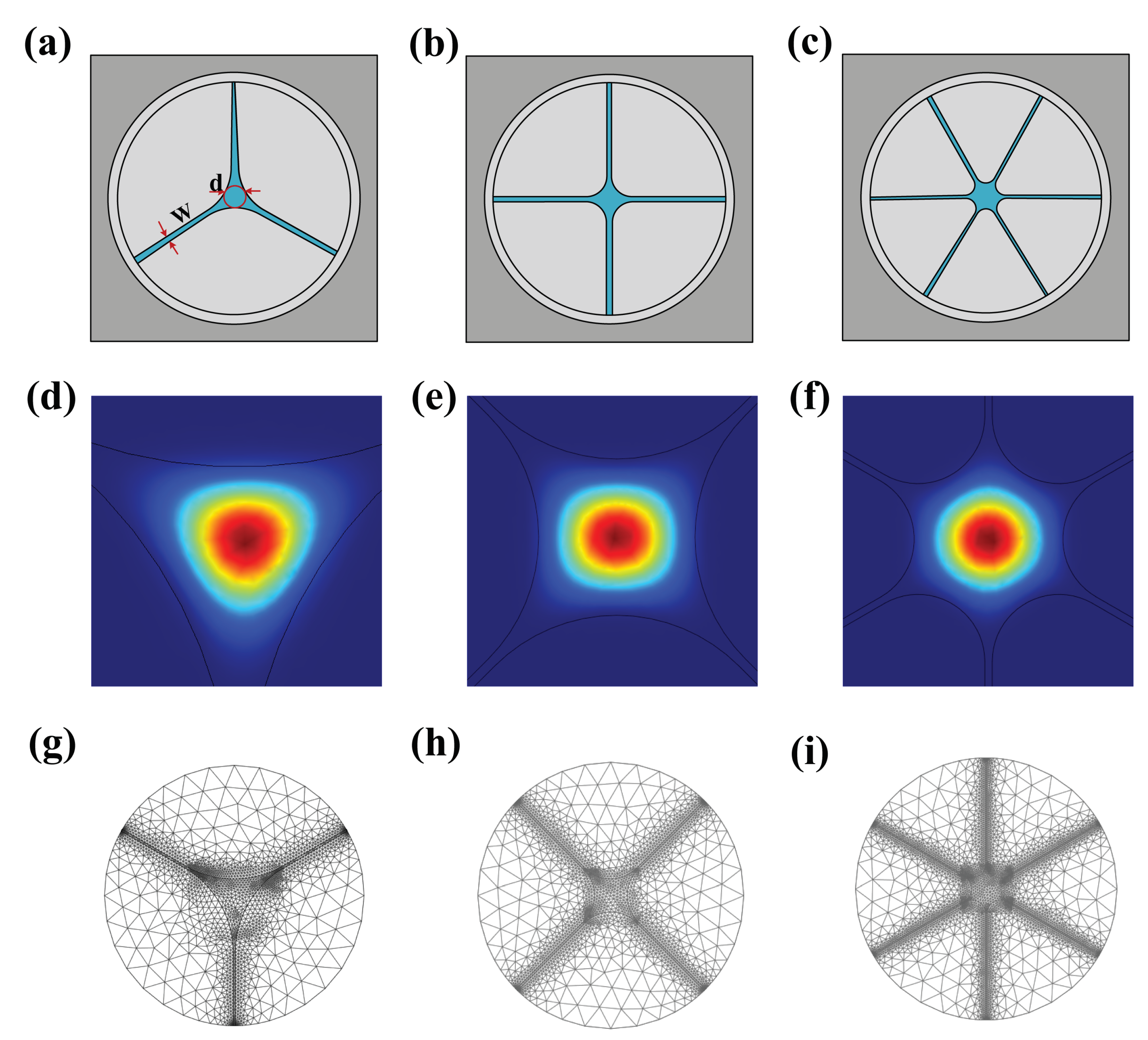
Figure 1.
(a–c) Cross section of the core area for simulation with three bridges, four bridges, and six bridges, respectively. (d–f) Fundamental optical mode field distribution of three bridges, four bridges, and six bridges, respectively. (g–i) Triangular mesh of finite element for the three brigades, four bridges, and six bridges SCF, respectively.
Figure 2.
(a) Computational flow of the proposed model. (b) Processing flow and structure diagram of a generative adversarial network for data augmentation, G is a typical encoder-decoder structure with 512, 256, 128, 128, 256, 512 neurons per layer (full-connection layer, from left to right), and D with 512, 256, 128, 64, 32, 1 neuron per layer (full-connection layer, from left to the right). (c) The structure of the back-propagation neural network for optical properties calculation has three hidden layers with 512 neurons each, one input layer and one output layer, the input layer corresponds to the four geometric features of the SCF, and the output layer corresponds to the optical properties to be calculated.
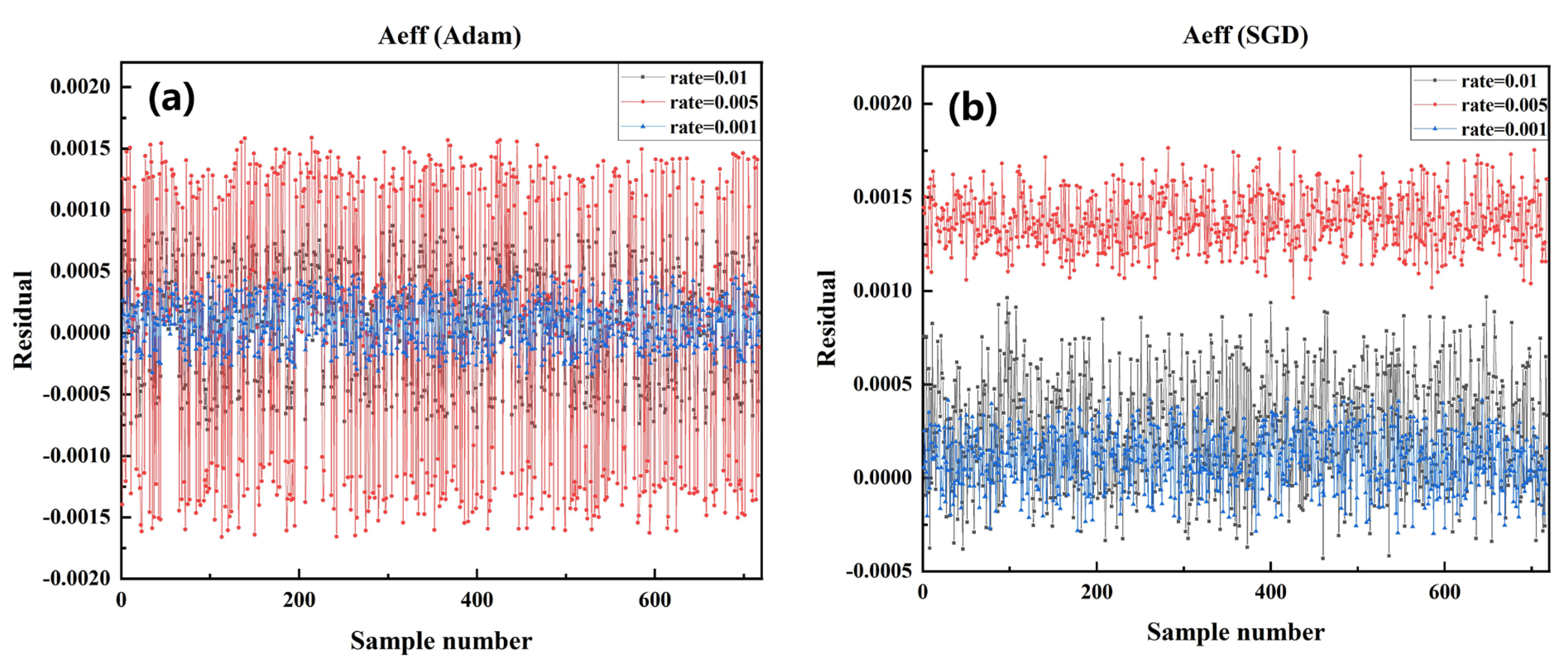
Figure 3.
Comparison of the residual between the predicted value and the actual value of in the test data set of the model trained by each algorithm under different learning rates in SGD optimizer and Adam optimizer. (a) Adam optimizer, LR: 0.01, 0.001, 0.005 (b) SGD optimizer, LR: 0.01, 0.001, 0.005.
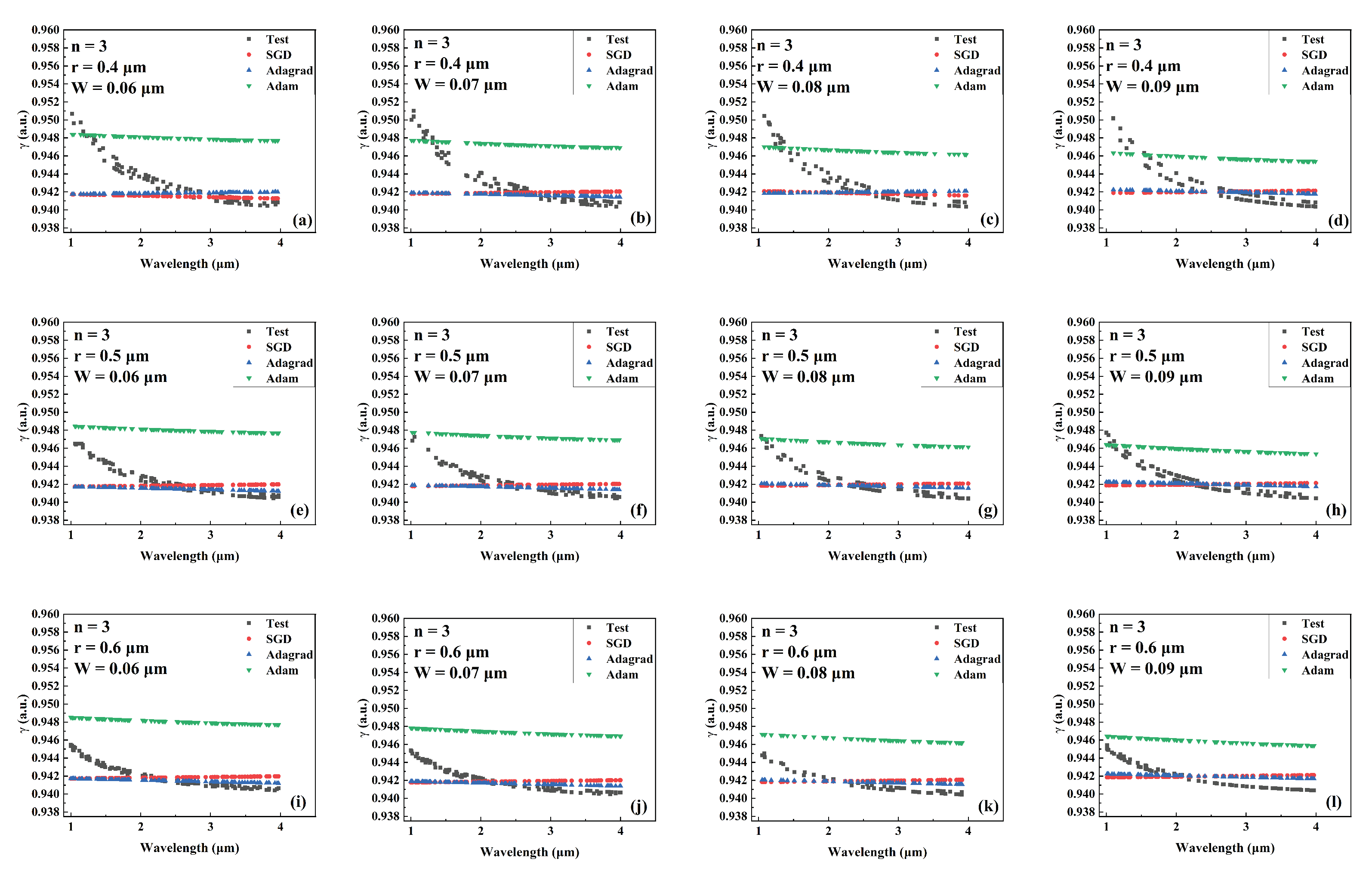
Figure 4.
Comparison of the predicted and actual values of in the test data set of the network model trained by different optimizers for different combinations of core radius and cantilever width (number of cantilevers: 3). (a) r = 0.4 m, W = 0.06 m. (b) r = 0.4 m, W = 0.07 m. (c) r = 0.4 m, W = 0.08 m. (d) r = 0.4 m, W = 0.09 m. (e) r = 0.5 m, W = 0.06 m. (f) r = 0.5 m, W = 0.07 m. (g) r = 0.5 m, W = 0.08 m. (h) r = 0.5 m, W = 0.09 m. (i) r = 0.6 m, W = 0.06 m. (j) r = 0.6 m, W = 0.07 m. (k) r = 0.6 m, W = 0.08 m. (l) r = 0.6 m, W = 0.09 m.
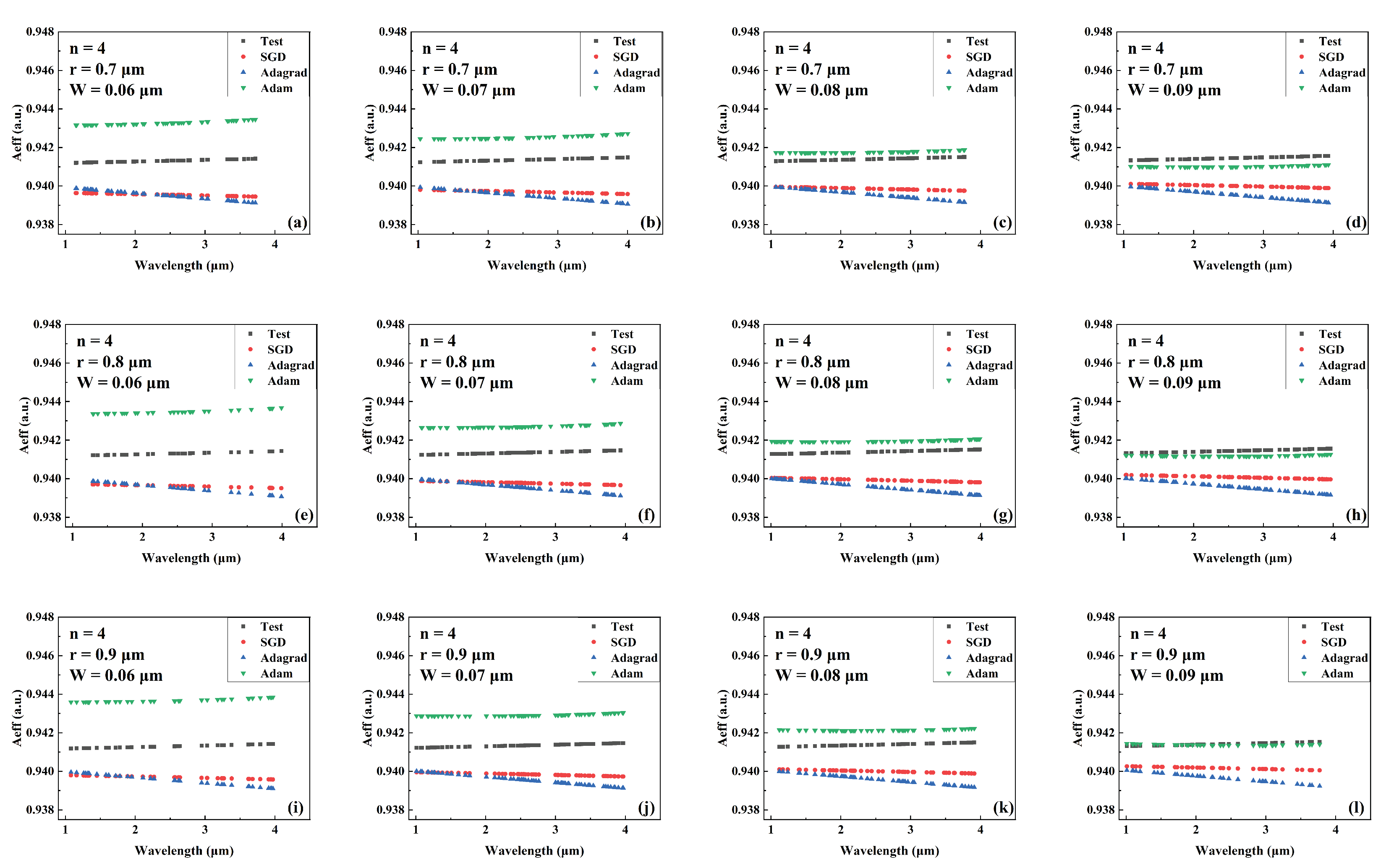
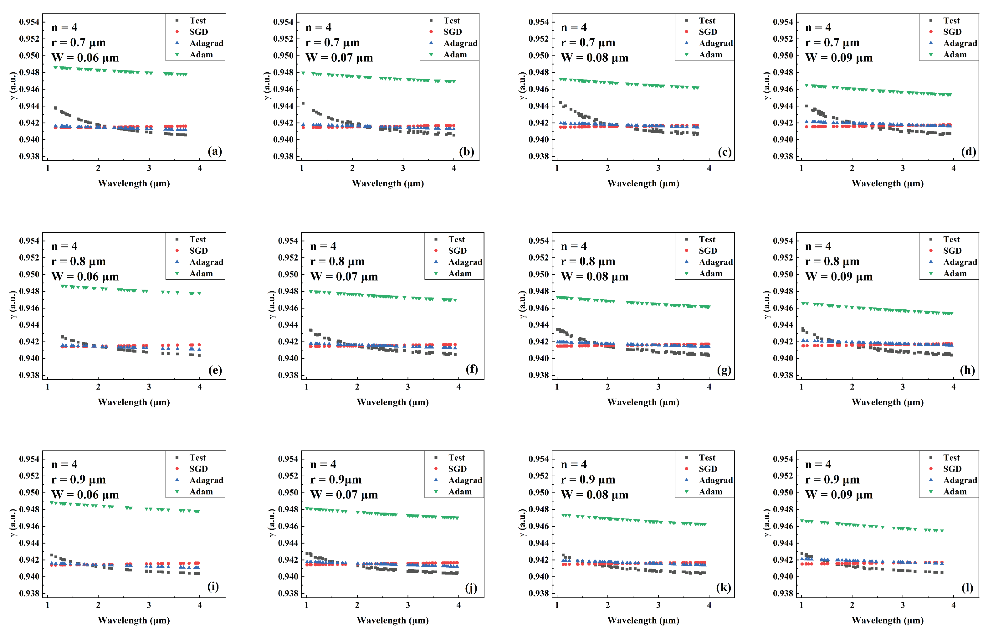
Figure 5.
Comparison of the predicted and actual values of in the test data set of the network model trained by different optimizers for different combinations of core radius and cantilever width (number of cantilevers: 4). (a) r = 0.7 m, W = 0.06 m. (b) r = 0.7 m, W = 0.07 m. (c) r = 0.7 m, W = 0.08 m. (d) r = 0.7 m, W = 0.09 m. (e) r = 0.8 m, W = 0.06 m. (f) r = 0.8 m, W = 0.07 m. (g) r = 0.8 m, W = 0.08 m. (h) r = 0.8 m, W = 0.09 m. (i) r = 0.9 m, W = 0.06 m. (j) r = 0.9 m, W = 0.07 m. (k) r = 0.9 m, W = 0.08 m. (l) r = 0.9 m, W = 0.09 m.
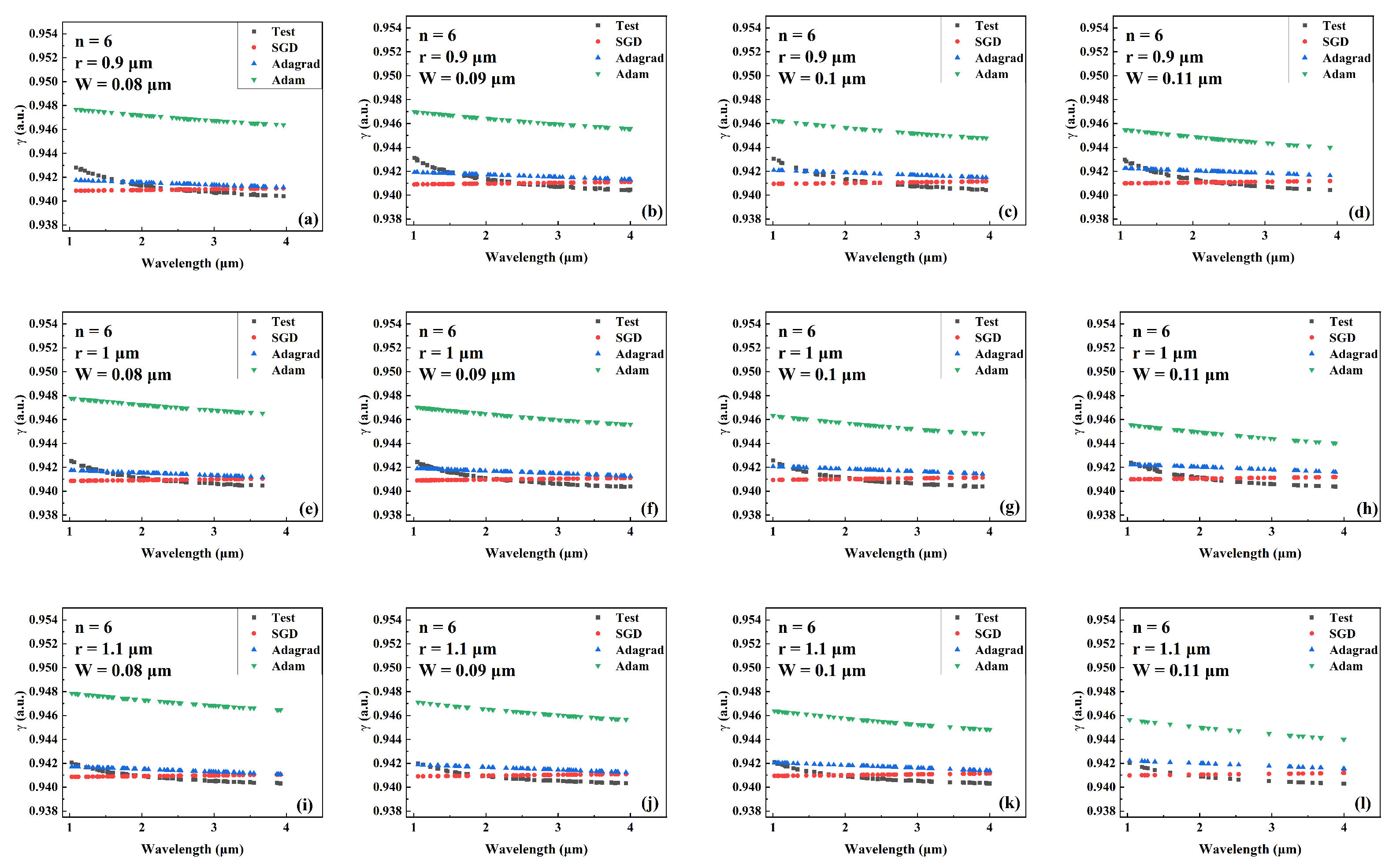
Figure 6.
Comparison of the predicted and actual values of in the test data set of the network model trained by different optimizers for different combinations of core radius and cantilever width (number of cantilevers: 6). (a) r = 0.9 m, W = 0.08 m. (b) r = 0.9 m, W = 0.09 m. (c) r = 0.9 m, W = 0.1 m. (d) r = 0.9 m, W = 0.11 m. (e) r = 1 m, W = 0.08 m. (f) r = 1 m, W = 0.09 m. (g) r = 1 m, W = 0.1 m. (h) r = 1 m, W = 0.11 m. (i) r = 1.1 m, W = 0.08 m. (j) r = 1.1 m, W = 0.09 m. (k) r = 1.1 m, W = 0.1 m. (l) r = 1.1 m, W = 0.11 m.
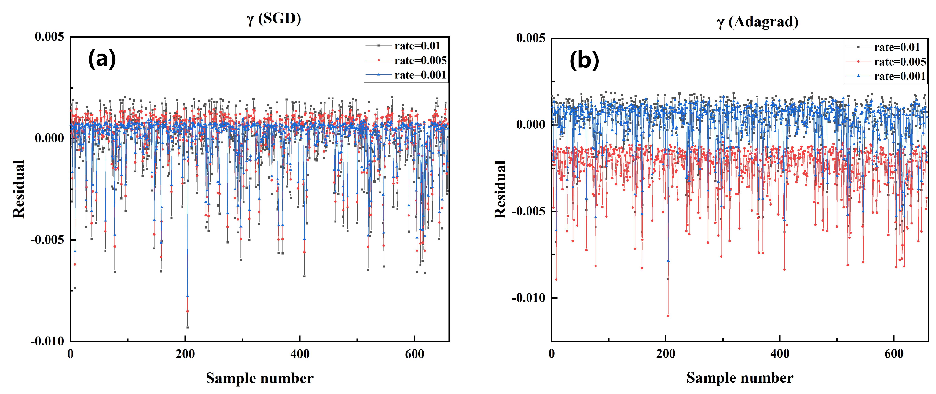
Figure 7.
Comparison of the residual between the predicted value and the actual value of in the test data set of the model trained by each algorithm under different learning rates in SGD optimizer and Adam optimizer. (a) SGD optimizer, LR: 0.01, 0.001, 0.005 (b) Adagrad optimizer, LR: 0.01, 0.001, 0.005.
Figure 8.
Comparison the predicted and actual values of in the test data set of the network model trained by different optimizers for different combinations of core radius and cantilever width (number of cantilevers: 3). (a) r = 0.4 m, W = 0.06 m. (b) r = 0.4 m, W = 0.07 m. (c) r = 0.4 m, W = 0.08 m. (d) r = 0.4 m, W = 0.09 m. (e) r = 0.5 m, W = 0.06 m. (f) r = 0.5 m, W = 0.07 m. (g) r = 0.5 m, W = 0.08 m. (h) r = 0.5 m, W = 0.09 m. (i) r = 0.6 m, W = 0.06 m. (j) r = 0.6 m, W = 0.07 m. (k) r = 0.6 m, W = 0.08 m. (l) r = 0.6 m, W = 0.09 m.
Figure 9.
Comparision the predicted and actual values of in the test data set of the network model trained by different optimizers for different combinations of core radius and cantilever width (number of cantilevers: 4). (a) r = 0.7 m, W = 0.06 m. (b) r = 0.7 m, W = 0.07 m. (c) r = 0.7 m, W = 0.08 m. (d) r = 0.7 m, W = 0.09 m. (e) r = 0.8 m, W = 0.06 m. (f) r = 0.8 m, W = 0.07 m. (g) r = 0.8 m, W = 0.08 m. (h) r = 0.8 m, W = 0.09 m. (i) r = 0.9 m, W = 0.06 m. (j) r = 0.9 m, W = 0.07 m. (k) r = 0.9 m, W = 0.08 m. (l) r = 0.9 m, W = 0.09 m.
Figure 10.
Comparison the predicted and actual values of in the test data set of the network model trained by different optimizers for different combinations of core radius and cantilever width (number of cantilevers: 6). (a) r = 0.9 m, W = 0.08 m. (b) r= 0.9 m, W = 0.09 m. (c) r = 0.9 m, W = 0.1 m. (d) r = 0.9 m, W = 0.11 m. (e) r = 1 m, W = 0.08 m. (f) r = 1 m, W = 0.09 m. (g) r = 1 m, W = 0.1 m. (h) r = 1 m, W = 0.11 m. (i) r = 1.1 m, W = 0.08 m. (j) r = 1.1 m, W = 0.09 m. (k) r = 1.1 m, W = 0.1 m. (l) r = 1.1 m, W = 0.11 m.
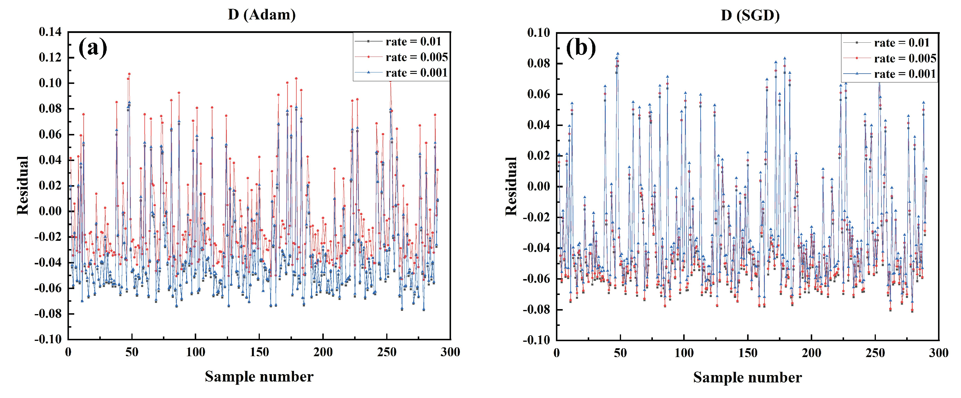
Figure 11.
Comparison of the residual between the predicted value and the actual value of D in the test data set of the model trained by each algorithm under different learning rates in SGD optimizer and Adam optimizer. (a) SGD optimizer, LR: 0.01, 0.001, 0.005 (b) Adam optimizer, LR: 0.01, 0.001, 0.005.
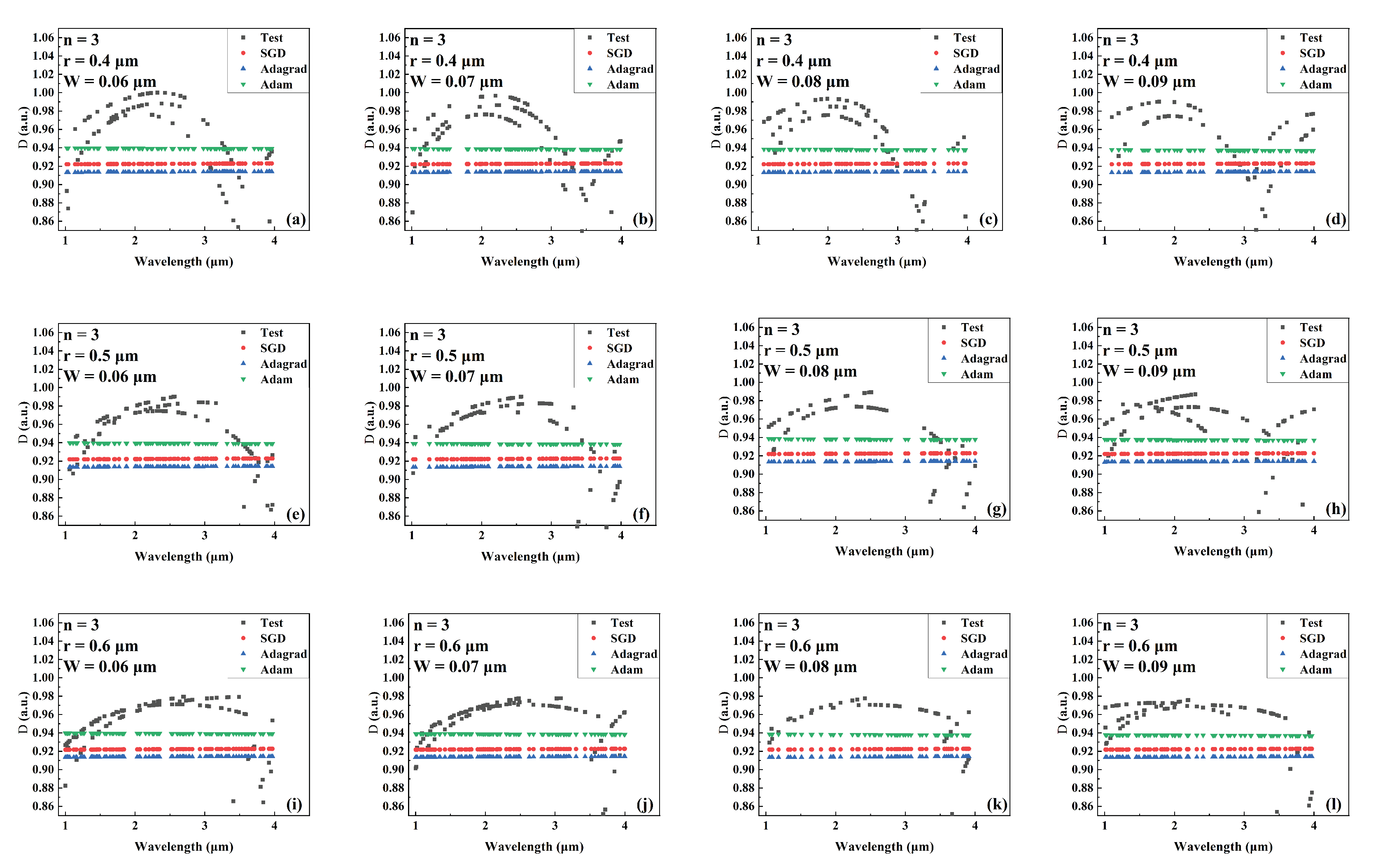
Figure 12.
Comparison the predicted and actual values of D in the test data set of the network model trained by different optimizers for different combinations of core radius and cantilever width (number of cantilevers: 3). (a) r = 0.4 m, W = 0.06 m. (b) r = 0.4 m, W = 0.07 m. (c) r = 0.4 m, W = 0.08 m. (d) r = 0.4 m, W = 0.09 m. (e) r = 0.5 m, W = 0.06 m. (f) r = 0.5 m, W = 0.07 m. (g) r = 0.5 m, W = 0.08 m. (h) r = 0.5 m, W = 0.09 m. (i) r = 0.6 m, W = 0.06 m. (j) r = 0.6 m, W = 0.07 m. (k) r = 0.6 m, W = 0.08 m. (l) r = 0.6 m, W = 0.09 m.
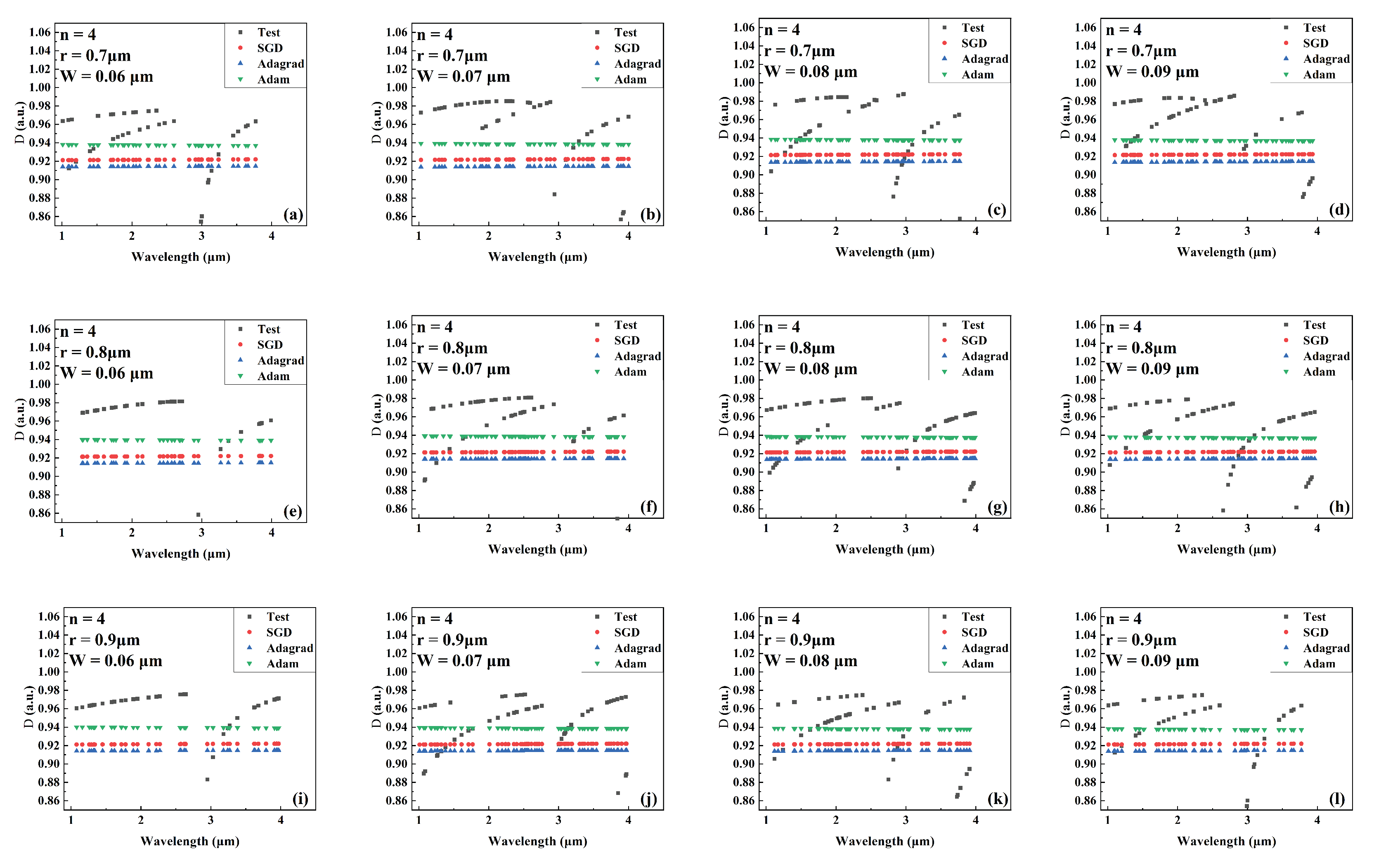
Figure 13.
Comparison the predicted and actual values of D in the test data set of the network model trained by different optimizers for different combinations of core radius and cantilever width (number of cantilevers: 4). (a) r = 0.7 m, W = 0.06 m. (b) r = 0.7 m, W = 0.07 m. (c) r = 0.7 m, W = 0.08 m. (d) r = 0.7 m, W = 0.09 m. (e) r = 0.8 m, W = 0.06 m. (f) r = 0.8 m, W = 0.07 m. (g) r = 0.8 m, W = 0.08 m. (h) r = 0.8 m, W = 0.09 m. (i) r = 0.9 m, W = 0.06 m. (j) r = 0.9 m, W = 0.07 m. (k) r = 0.9 m, W = 0.08 m. (l) r = 0.9 m, W = 0.09 m.
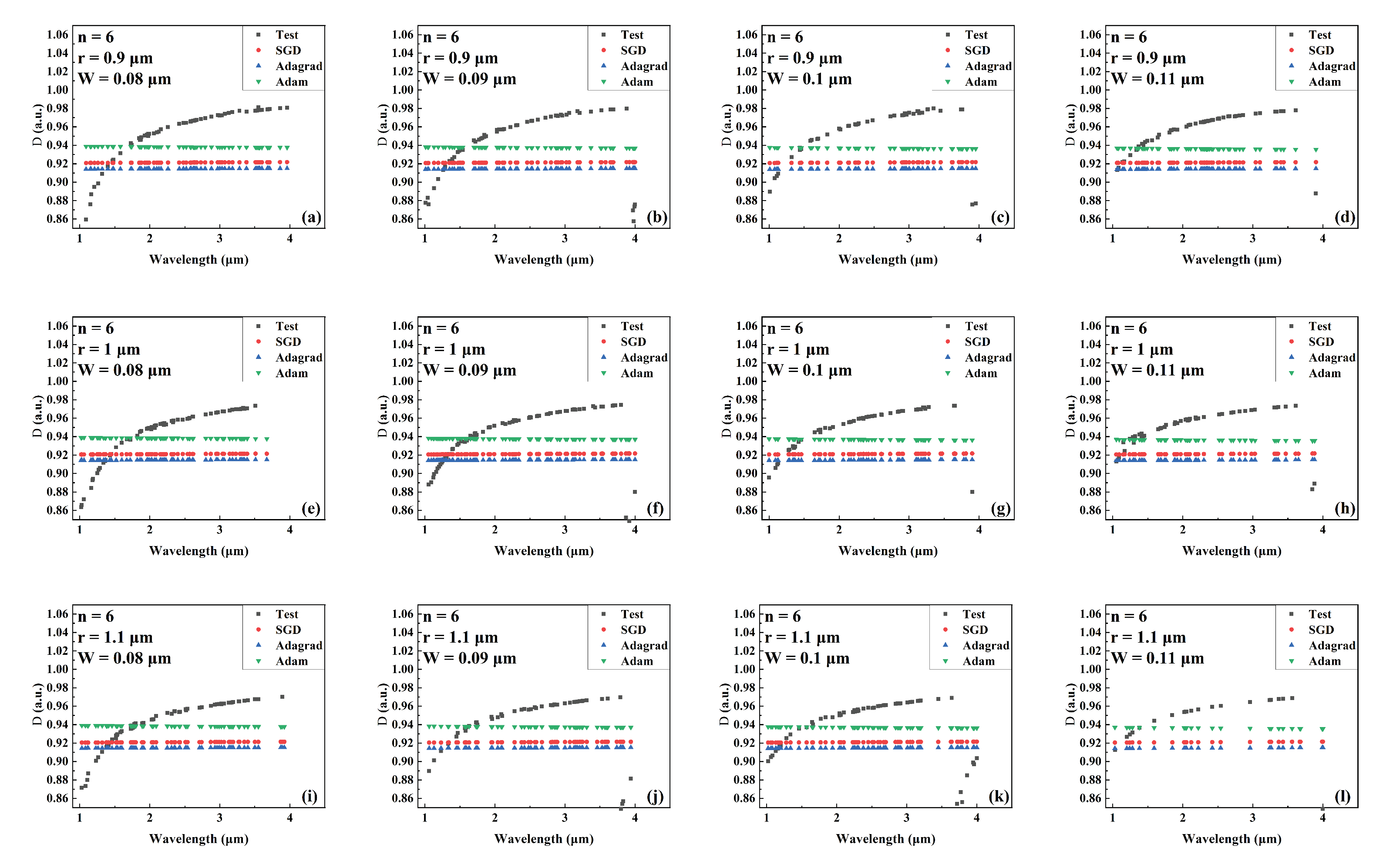
Figure 14.
Comparision the predicted and actual values of D in the test data set of the network model trained by different optimizers for different combinations of core radius and cantilever width (number of cantilevers: 6). (a) r = 0.9 m, W = 0.08 m. (b) r = 0.9 m, W = 0.09 m. (c) r = 0.9 m, W = 0.1 m. (d) r = 0.9 m, W = 0.11 m. (e) r = 1 m, W = 0.08 m. (f) r = 1 m, W = 0.09 m. (g) r = 1 m, W = 0.1 m. (h) r = 1 m, W = 0.11 m. (i) r = 1.1 m, W = 0.08 m. (j) r = 1.1 m, W = 0.09 m. (k) r = 1.1 m, W = 0.1 m. (l) r = 1.1 m, W = 0.11 m.
Table 1.
Average mean square deviation of a neural network model of training process and verification process under different learning rates and optimizers.
Table 1.
Average mean square deviation of a neural network model of training process and verification process under different learning rates and optimizers.
| Optimizer | LR | MSE (Training, a.u.) | MSE (Validation, a.u.) |
|---|
| SGD | 0.01 | 0.0061 | 0.0043 |
| 0.005 | 0.0058 | 0.0043 |
| 0.001 | 0.0064 | 0.0043 |
| Adagrad | 0.01 | 0.0054 | 0.0043 |
| 0.005 | 0.0069 | 0.0046 |
| 0.001 | 0.0008 | 0.0044 |
| Adam | 0.01 | 0.0108 | 0.0044 |
| 0.005 | 0.0057 | 0.0046 |
| 0.001 | 0.0052 | 0.0043 |
Table 2.
Performance evaluation results for predictions of on the test dataset with models trained with different training configuration.
Table 2.
Performance evaluation results for predictions of on the test dataset with models trained with different training configuration.
| Optimizer | LR | MSE (×, a.u.) | RMSE (a.u.) | MAE (a.u.) |
|---|
| SGD | 0.01 | 1.63 | 0.0004 | 0.0003 |
| 0.005 | 1.91 | 0.0014 | 0.0014 |
| 0.001 | 3.78 | 0.0002 | 0.0002 |
| Adagrad | 0.01 | 2.38 | 0.0049 | 0.0049 |
| 0.005 | 4.92 | 0.0022 | 0.0022 |
| 0.001 | 8.01 | 0.0028 | 0.0028 |
| Adam | 0.01 | 2.17 | 0.0005 | 0.0004 |
| 0.005 | 1.13 | 0.0011 | 0.0009 |
| 0.001 | 0.51 | 0.0002 | 0.0002 |
Table 3.
Average of each model on evaluation metrics when predicting in the test dataset under different combinations of parameters.
Table 3.
Average of each model on evaluation metrics when predicting in the test dataset under different combinations of parameters.
| Optimizer | MSE (×, a.u.) | RMSE (a.u.) | MAE (a.u.) |
|---|
| SGD | 0.0704 | 0.00066 | 0.00062 |
| Adagrad | 5.10 | 0.0033 | 0.0033 |
| Adam | 0.467 | 0.00058 | 0.0005 |
Table 4.
Performance evaluation results for predictions of on test datasets with models trained with different optimizers and different LRs.
Table 4.
Performance evaluation results for predictions of on test datasets with models trained with different optimizers and different LRs.
| Optimizer | LR | MSE (×, a.u.) | RMSE (a.u.) | MAE (a.u.) |
|---|
| SGD | 0.01 | 2.87 | 0.0017 | 0.0012 |
| 0.005 | 1.85 | 0.0014 | 0.0010 |
| 0.001 | 1.2 | 0.0011 | 0.0007 |
| Adagrad | 0.01 | 2.39 | 0.0015 | 0.0011 |
| 0.005 | 7.82 | 0.0028 | 0.0024 |
| 0.001 | 1.66 | 0.0013 | 0.0010 |
| Adam | 0.01 | 6.92 | 0.0026 | 0.0025 |
| 0.005 | 8.06 | 0.0028 | 0.0025 |
| 0.001 | 4.37 | 0.0021 | 0.0016 |
Table 5.
Average of each model on evaluation metrics when predicting in the test dataset under different combinations of parameters.
Table 5.
Average of each model on evaluation metrics when predicting in the test dataset under different combinations of parameters.
| Optimizer | MSE (×, a.u.) | RMSE (a.u.) | MAE (a.u.) |
|---|
| SGD | 1.97 | 0.0014 | 0.001 |
| Adagrad | 3.96 | 0.0019 | 0.0015 |
| Adam | 6.45 | 0.0025 | 0.0022 |
Table 6.
Performance evaluation results for predictions of D on the test dataset with models trained with different optimizers and different LRs.
Table 6.
Performance evaluation results for predictions of D on the test dataset with models trained with different optimizers and different LRs.
| Optimizer | LR | MSE (a.u.) | RMSE (a.u.) | MAE (a.u.) |
|---|
| SGD | 0.01 | 0.01366 | 0.11686 | 0.06026 |
| 0.005 | 0.01421 | 0.11920 | 0.08287 |
| 0.001 | 0.01349 | 0.11614 | 0.06438 |
| Adagrad | 0.01 | 0.01455 | 0.12061 | 0.05501 |
| 0.005 | 0.01350 | 0.11617 | 0.06380 |
| 0.001 | 0.01367 | 0.11692 | 0.07498 |
| Adam | 0.01 | 0.01354 | 0.011638 | 0.06264 |
| 0.005 | 0.01347 | 0.11604 | 0.06417 |
| 0.001 | 0.01345 | 0.11602 | 0.06414 |
Table 7.
Average of each model on evaluation metrics when predicting D in the test dataset under different combinations of parameters.
Table 7.
Average of each model on evaluation metrics when predicting D in the test dataset under different combinations of parameters.
| Optimizer | MSE (a.u.) | RMSE (a.u.) | MAE (a.u.) |
|---|
| SGD | 0.01378 | 0.11740 | 0.06917 |
| Adagrad | 0.01390 | 0.11790 | 0.06460 |
| Adam | 0.01350 | 0.11617 | 0.06445 |
Table 8.
MSE averages for models trained using different training configurations (optimizer and LR) predict different optical properties, the bold denotes the optimal in this prediction.
Table 8.
MSE averages for models trained using different training configurations (optimizer and LR) predict different optical properties, the bold denotes the optimal in this prediction.
| Optimizer | LR | (× ) | (× ) | D (× ) |
|---|
| SGD | 0.01 | 1.63 | 2.87 | 1.366 |
| 0.005 | 1.91 | 1.85 | 1.421 |
| 0.001 | 3.78 | 1.2 | 1.349 |
| Adagrad | 0.01 | 2.38 | 2.39 | 1.455 |
| 0.005 | 4.92 | 7.82 | 1.350 |
| 0.001 | 8.01 | 1.66 | 1.367 |
| Adam | 0.01 | 2.17 | 6.92 | 1.354 |
| 0.005 | 1.13 | 8.06 | 1.347 |
| 0.001 | 0.51 | 4.37 | 1.345 |


