
A Universal Testbed for IoT Wireless Technologies: Abstracting Latency, Error Rate and Stability from the IoT Protocol and Hardware Platform

 ,
,  ,
,  and
and 
Abstract
:1. Introduction
2. Universal Testbed
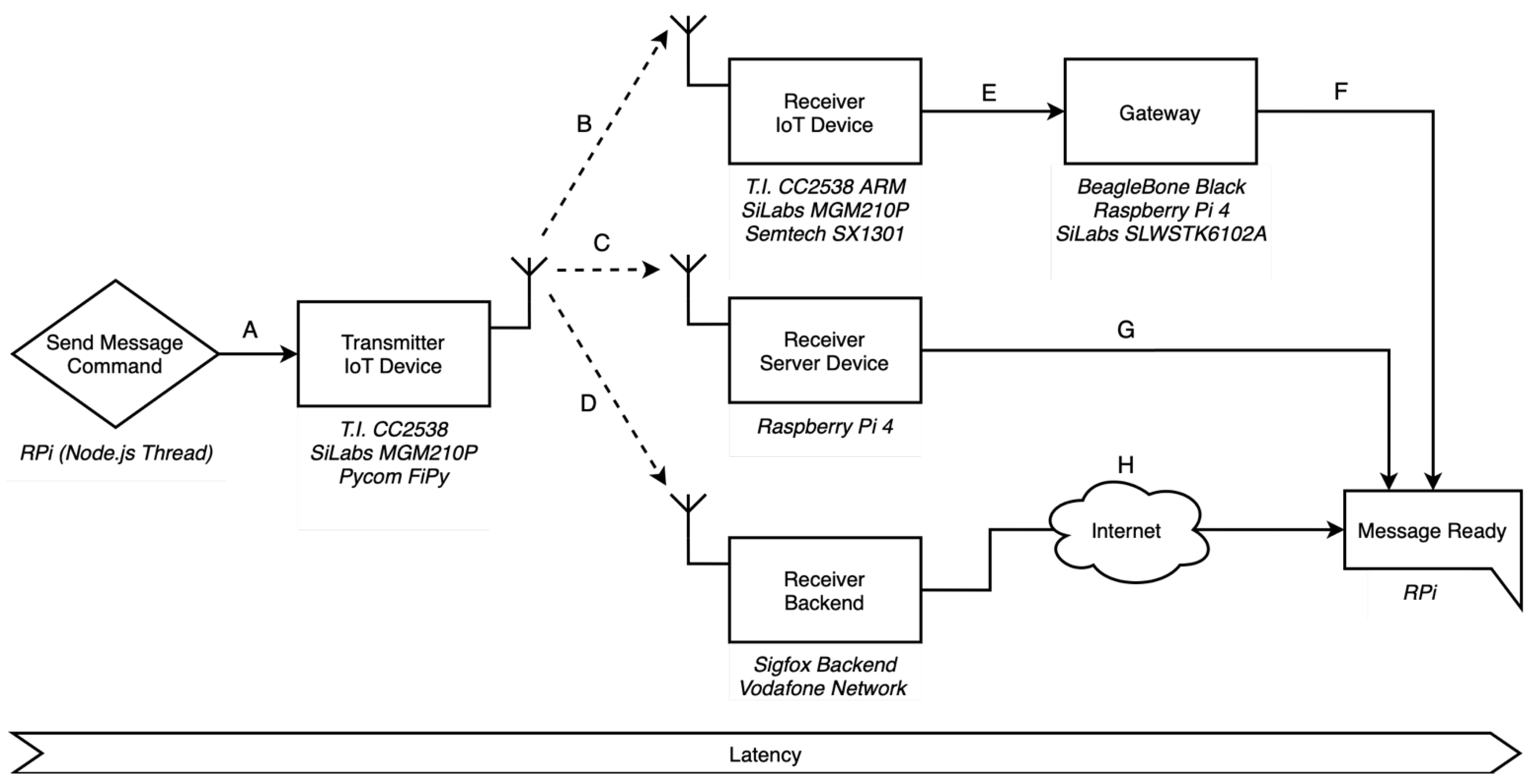
2.1. Latency and Laboratory Workaround
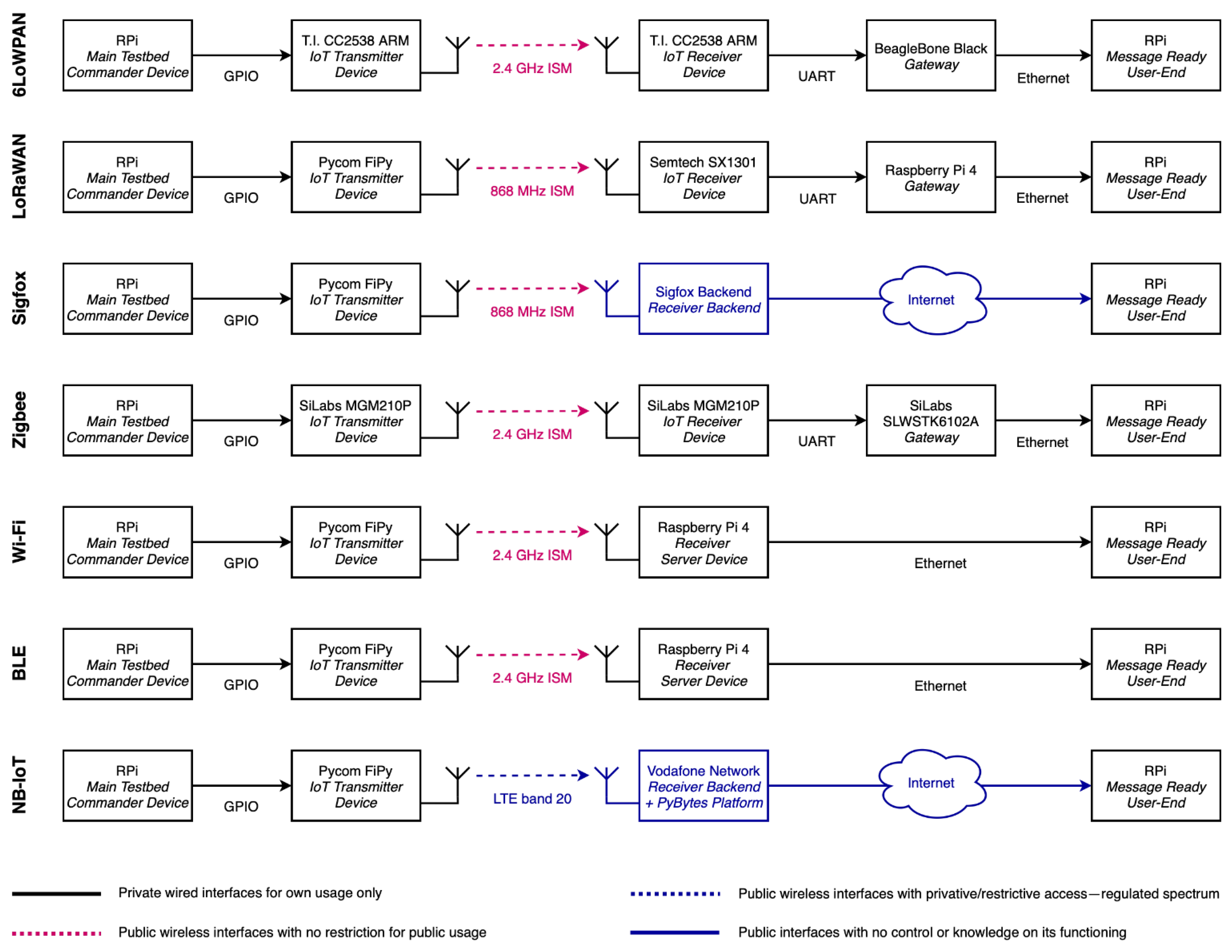
- A-B-E-F: 6LoWPAN, ZigBee, LoRaWAN
- A-D-H: Sigfox, NB-IoT
- A-C-G: Wi-Fi, BLE
The Transmitter IoT Device’s Firmware
2.2. Considerations Regarding Different Wireless Technologies
- Sigfox: The message payload was always set to be 12 bytes—the maximum allowed;
- LoRaWAN: is the most common configuration of Spreading Factor (SF7), and bandwidth (125 kHz) was used;
- BLE: We used advertisements to spread the message (two transmissions for each message). We did this because several problems were encountered in timing, and too many losses appeared when advertising only once—too many even to consider BLE an IoT technology. However, we attribute this to the fact of not being able to use point-to-point messages and only advertisements, and advertisements were the only BL- supported feature by Pycom at the time of doing this work;
- NB-IoT: We used Vodafone SIM card, i.e., Vodafone LTE network, with the layer of Pycom Pybytes as a backend for receiving messages;
- Wi-Fi: Hypertext transfer protocol (HTTP) was used as the application layer to send messages as it is an utterly common layer in Wi-Fi utilisation;
- 6LoWPAN: User datagram protocol (UPD) was used as the top layer to send messages;
- Zigbee: The clean Zigbee stack was used.
2.3. The Testbed’s Interface
2.3.1. Start Test (Route: POST /start/{idtech}/period/{period}/limit/{limit})
- idtech is an integer designating the wireless IoT technology under test (required);
- period is the period between transmissions in milliseconds (defaults to 10,000);
- limit is the message limit (defaults to 100).
2.3.2. Print Current Results (Route: GET /print)
2.3.3. Stop Test (Route: PUT/stop)
- Individual message data (fields identified by a numeral, from “0” to “999” in this example):
- start is the timestamp when the IoT transmitter device was called to send the message;
- successful is a Boolean indicating if the message properly arrived at its destination;
- end is the timestamp when the RPi received the call-back from the IoT receiver device—the moment when the latency trip is completed;
- timestamp is a timestamp recorded by some gateways when processing the messages (only for 6LoWPAN and LoRaWAN);
- latency is the difference between end and start, i.e., the latency of the message.
- Whole test data (field “testInfo”):
- testStart is the timestamp of the moment when the test began;
- testEnd is the timestamp of the moment when the test finished;
- limit is an integer indicating the number of messages defined in the test;
- top is the maximum sequence number achieved when performing the test—it should be limit–1 if the test goes well;
- period is the period between messages defined in the test configuration;
- idtech is an integer designating the wireless technology;
- avgLatency is the average latency for the whole test;
- minLatency is the minimum registered latency;
- maxLatency is the maximum registered latency;
- stdDev is the standard deviation for the cluster of latencies recorded in the test;
- outliers is the count of latencies out of avgLatency ±10%;
- outliersRel is the relative number of outliers with respect to top+1;
- errorCount is the messages lost count during the test;
- errorRate is the relative error rate—errorCount with respect to top+1;
- finishReason is the reason the test finished; usually, the test finishes because the message count (top) reaches its limit.
2.3.4. Callback (Route: POST /callback)
- idtech is an integer designating the wireless technology;
- seq is the message sequence number, useful to sort messages upon arrival, measure latency and determine losses;
- epoch_ms is the timestamp of the device under characterisation in milliseconds—however, this time is not used to calculate this kind of latency as the Testbed device uses its own time reference for that.
3. The Testbed’s Temporal Characterisation
- Stability responding to external interrupts (Section 3.1);
- Temporal stability of the internal clock (Section 3.2);
- Auto-delay when responding to self-events (Section 3.3).
3.1. The Testbed’s Reaction to External Interrupts
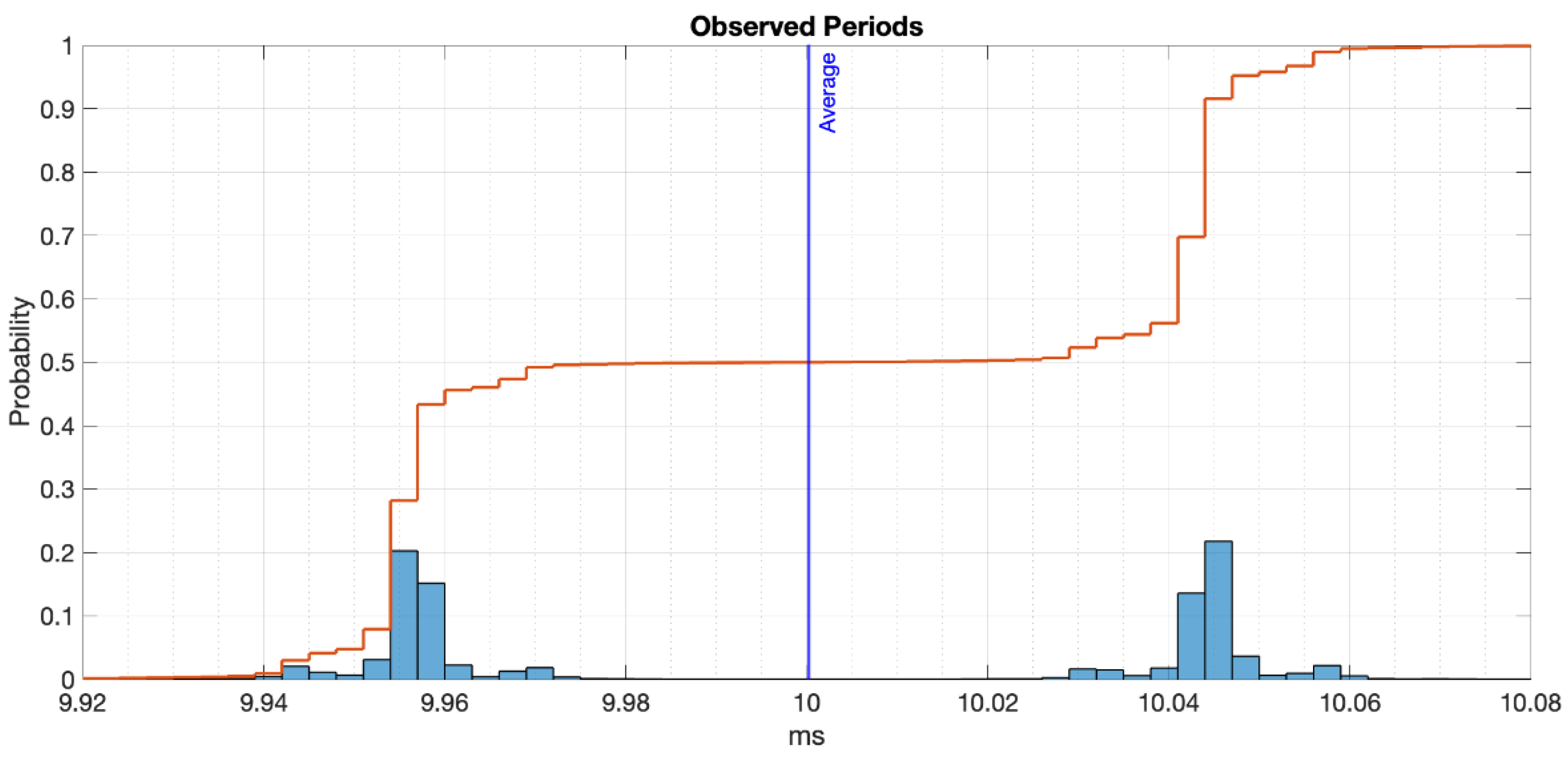
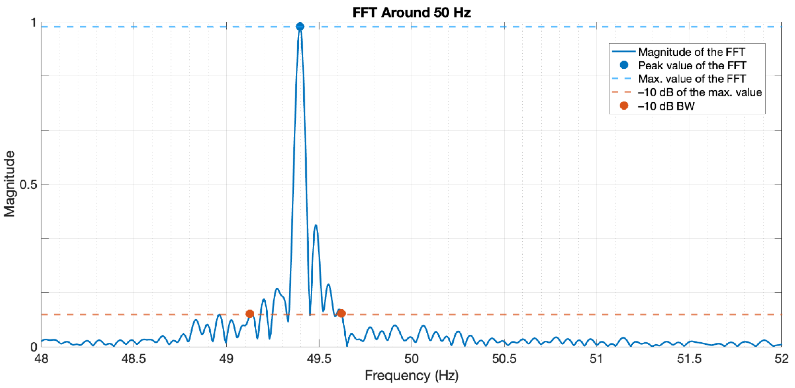
3.2. Temporal Stability of the Internal Clock
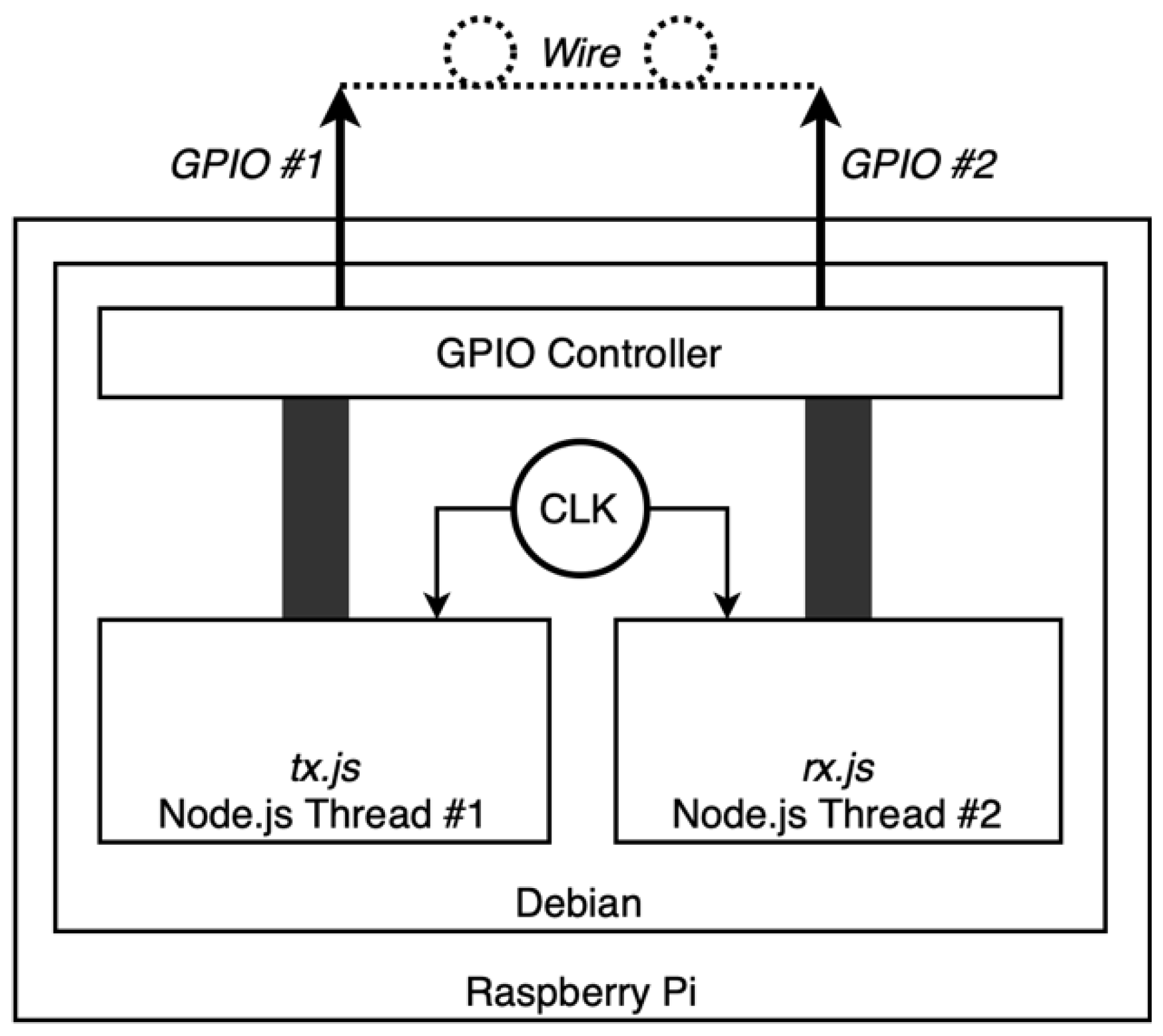
3.3. Self-Delay
- tx.js: this process toggles a GPIO digital state, which is connected to another GPIO of the RPi, firing the interrupt; it stores the timestamp of the toggling process as well in microseconds;
- rx.js: this process reacts to both rising and falling edge interrupts on the GPIO and stores the timestamp of the event in microseconds.
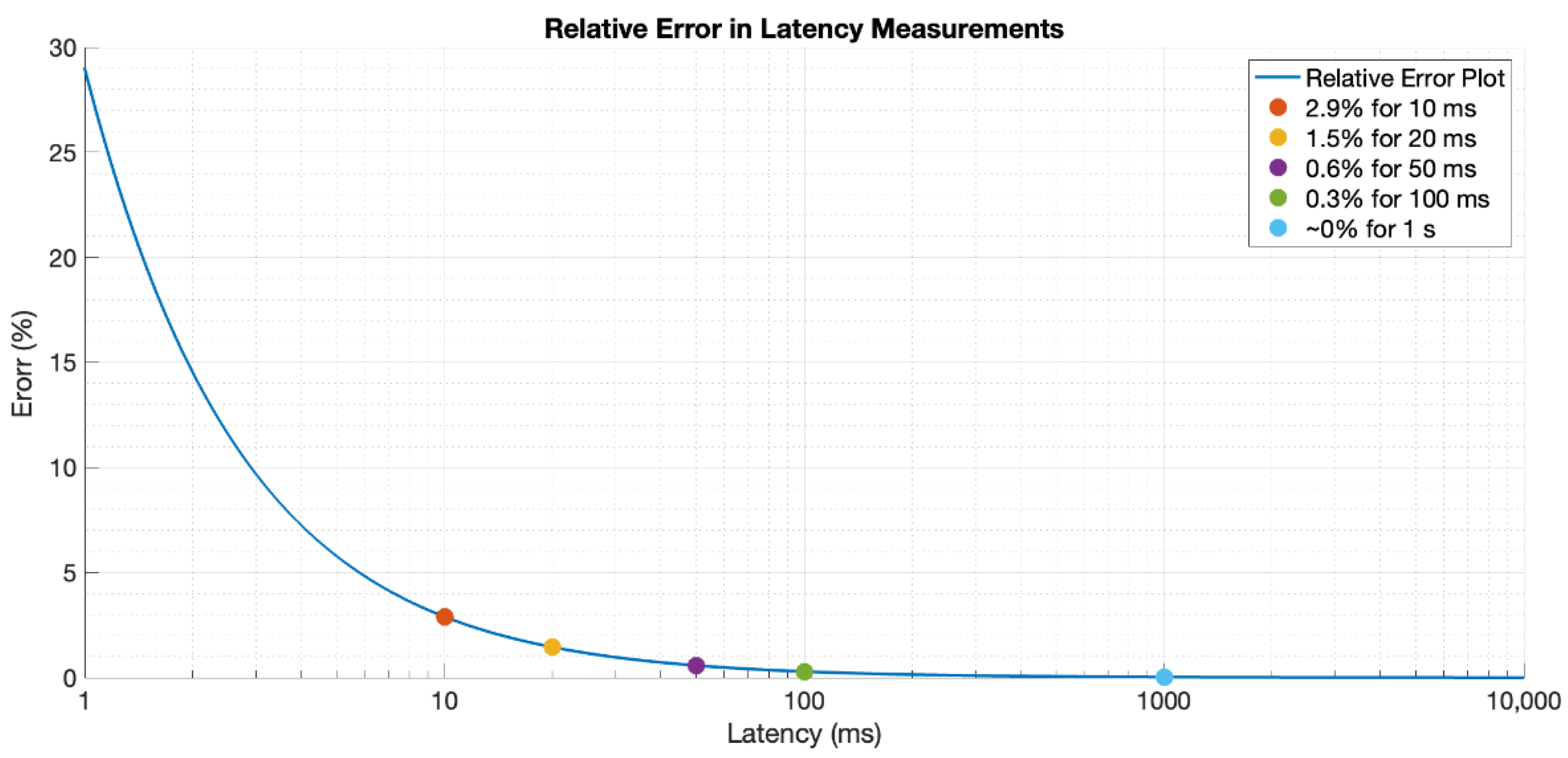
3.4. Testbed’s Error Range Validation
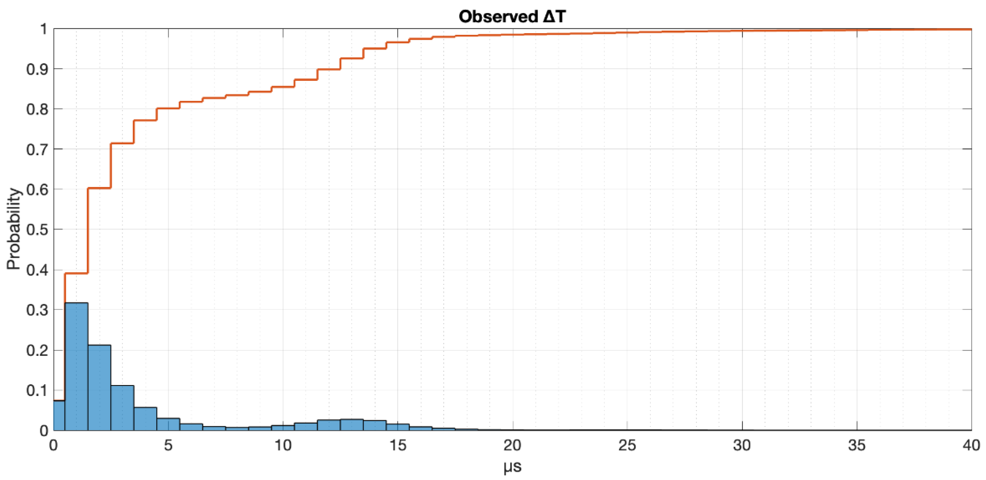
- External interrupts: the response to external interrupts seems to be very accurate and precise, with 90 % of drifting within 12 µs. Since we are working with latencies on the order of tens of milliseconds, we can consider this influence negligible (~0.1%).
- Internal clock: the internal clock presents an error in the order of hundreds of microseconds (240 µs), with 90% confidence values between 160 µs and 370 µs.
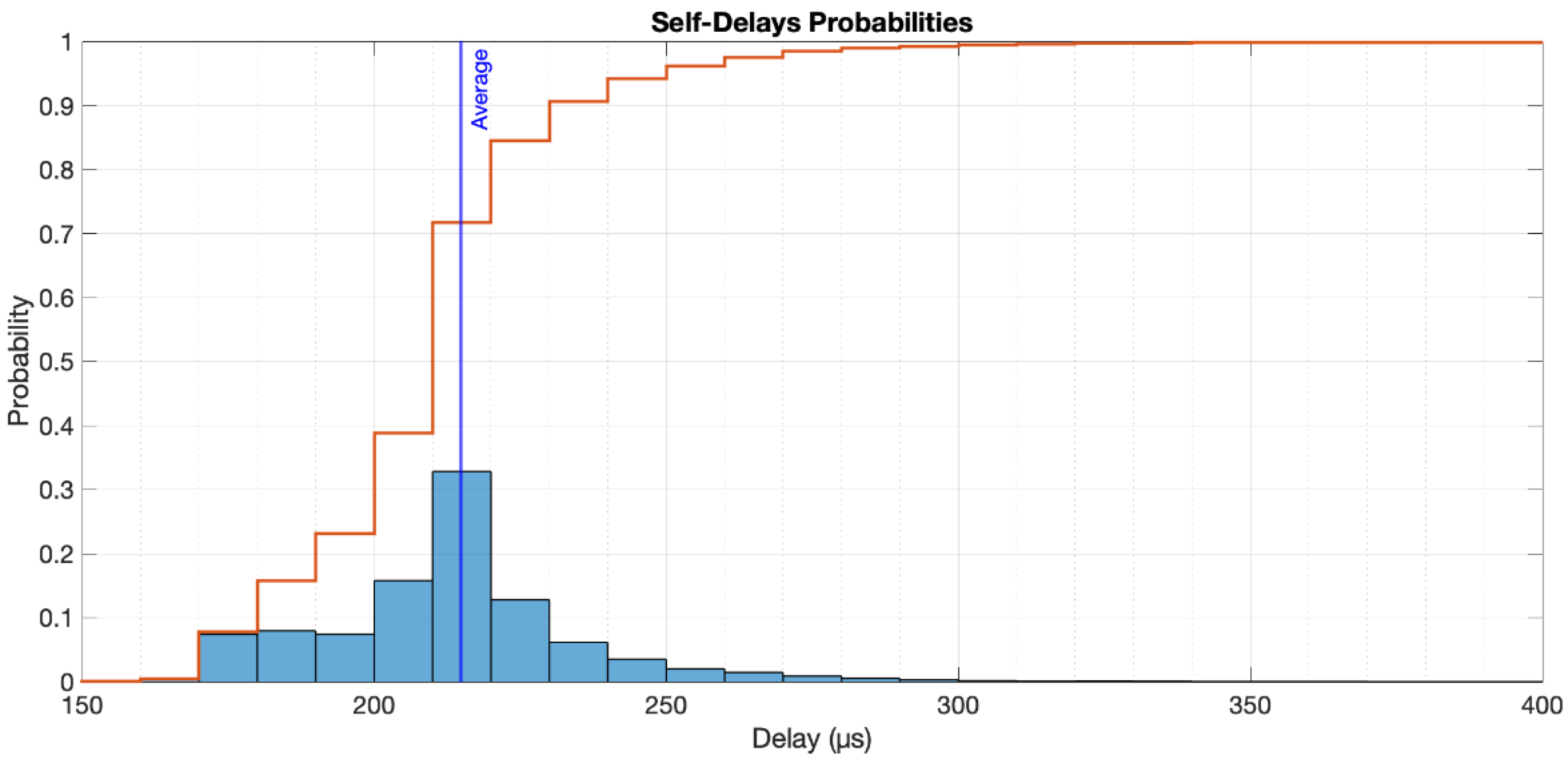
- Self-delay: the self-delay, which is probably the most important factor in our system since we are using the same Testbed to command external devices and measure time, has an average value around 215 µs, with a 90% confidence delay <240 µs and no values less than 160 µs.
- γ is the actual latency;
- φ is the measured latency;
- δ is the introduced metering error, which is, according to our characterisation, a value in the range of 320 µs and 610 µs.
4. Measurements and Results
4.1. Parameters: Latency, Error, Stability
- Latency: minimum, average, maximum;
- Error rate: message loss count (), relative error rate (E);
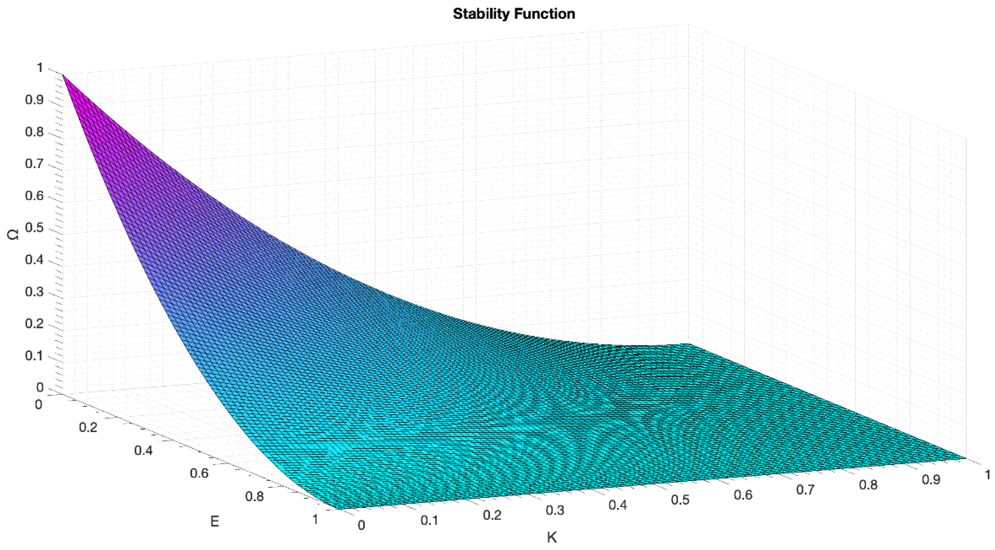
- Stability: standard deviation of latency (), messages out of average latency ± 10%—outliers, both in absolute count () and relative (K)—and a factor indicating a quality of stability () defined as in Equation (3) and Figure 8.
4.2. Real Tests
- 6LoWPAN: ML 10,000; PT 1
- LoRaWAN: ML 10,000; PT 1
- Sigfox: ML 100; PT 15
- Zigbee: ML 10,000; PT 1
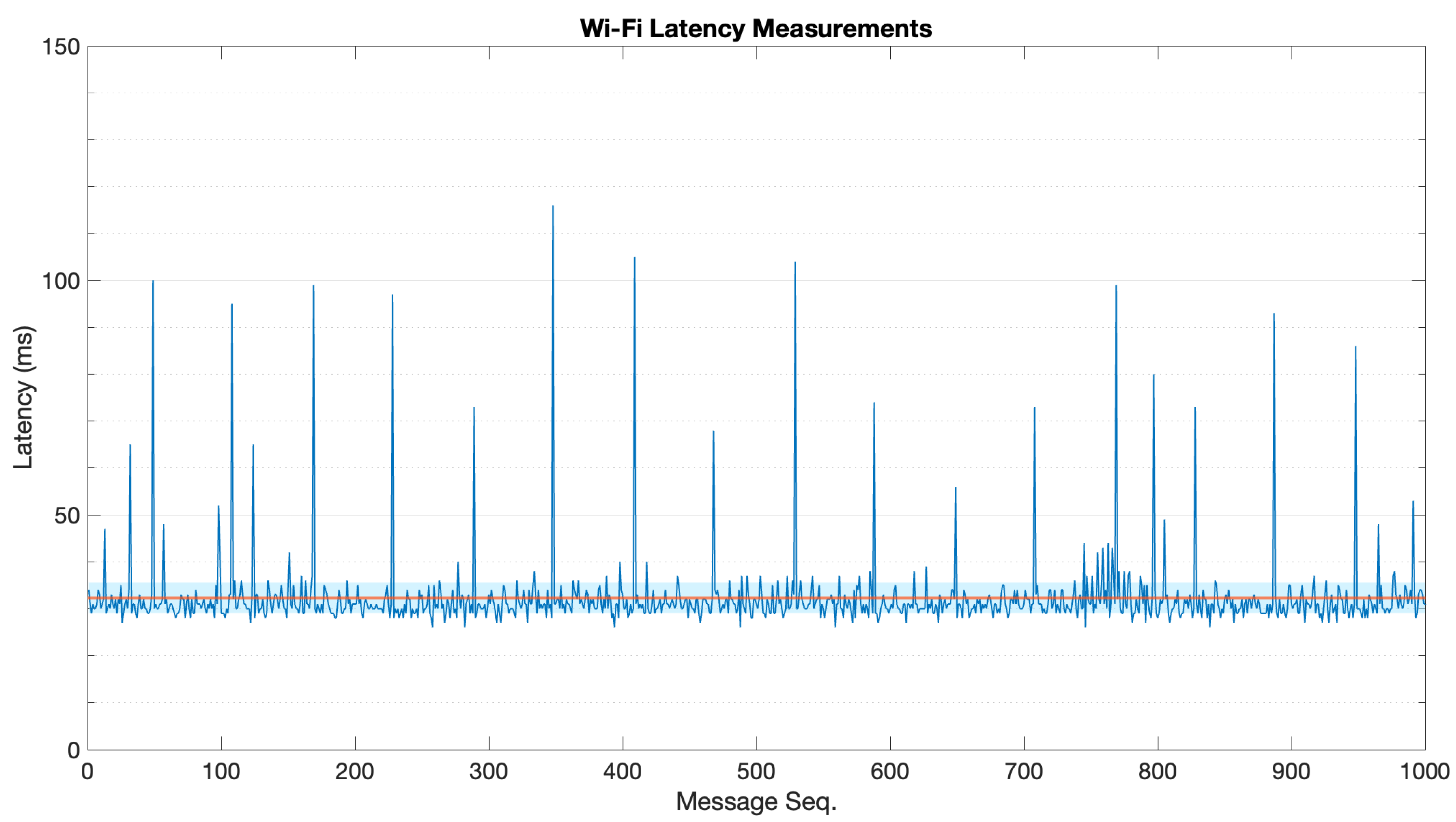
- Wi-Fi: ML 10,000; PT 1
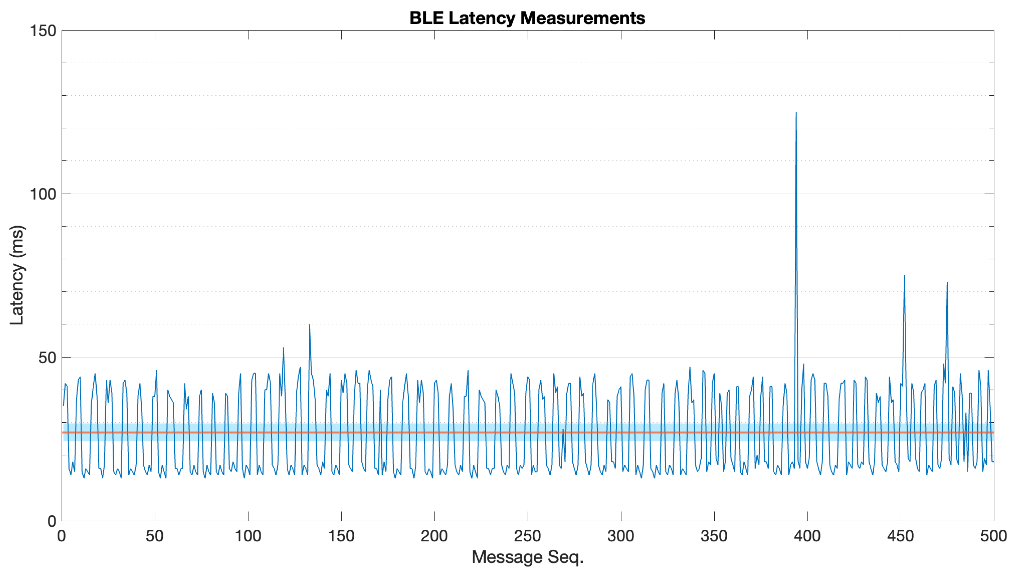
- BLE: ML 500; PT 10
- NB-IoT: ML 5000; PT 5
4.3. Results Discussion
- Zigbee: we used the whole Zigbee stack, which handles losses itself.
- Wi-Fi: we used HTTP, which works over Transmission Control Protocol (TCP) and therefore handles losses as well.
- BLE: as stated in Section 2.2 hereof, we advertised every message twice, so the chance for the message getting lost is negligible.
5. Conclusions
- Technology-agnostic: it has been designed to characterise any IoT wireless technology, with independence of the communication architecture and the protocols used;
- Cost, time, and resource efficient: it is based on the affordable Raspberry Pi board, and it can work on any Linux machine with a Node.js runtime;
- Portable and easy to deploy: the Testbed design allows its transportation and set up in any location;
- Replicable and scalable: based on standard HW and SW tools, it is easy to replicate, adapt and improve to measure other timing parameters.
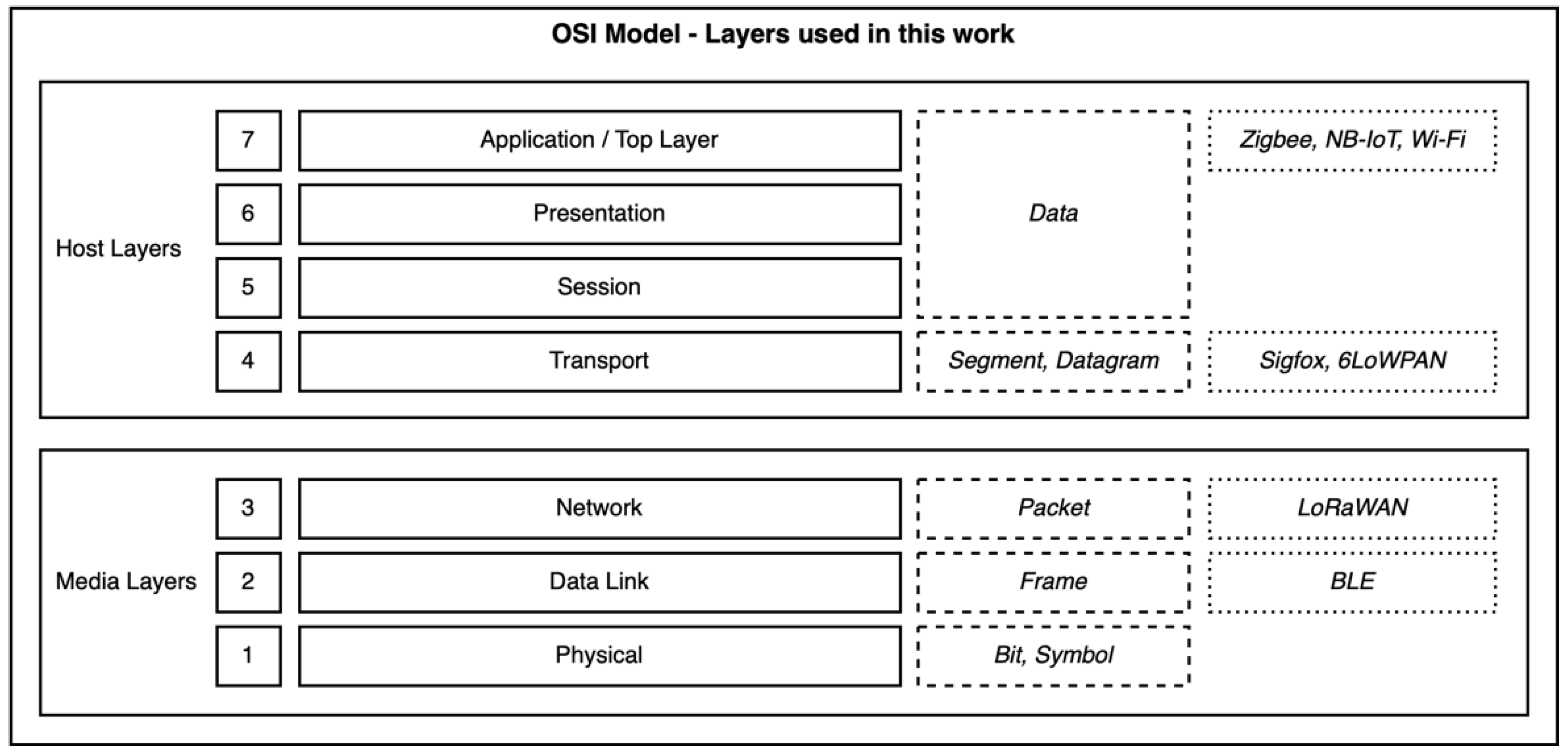
Future Sights
- Applications: Zigbee, NB-IoT, Wi-Fi (HTTP);
- Transport: Sigfox, 6LoWPAN (UDP);
- Network: LoRaWAN;
- Data Link: BLE (advertisements, two repetitions per message).
- Zigbee, Sigfox, LoRaWAN: due to their own nature and definition, those layers are the ones to use between the end device and the receiver on the RF link;
- BLE: the equipment used in this work (Pycom FiPy), only supported BLE advertisements when doing these tests—other manufacturers may provide support for upper layers;
- NB-IoT: at the moment of this work, we could only use Pybytes’ abstraction layer to send and receive NB-IoT messages; so, we are considering this the top layer.
Author Contributions
Funding
Institutional Review Board Statement
Informed Consent Statement
Data Availability Statement
Conflicts of Interest
Appendix A

Appendix B

References
- Wegner, P. Global IoT Spending to Grow 24% in 2021, Led by Investments in IoT Software and IoT Security. Available online: https://iot-analytics.com/2021-global-iot-spending-grow-24-percent/ (accessed on 14 April 2022).
- Evans, D. The Internet of Things. How the Next Evolution of the Internet Is Changing Everything. Available online: https://www.cisco.com/c/dam/en_us/about/ac79/docs/innov/IoT_IBSG_0411FINAL.pdf (accessed on 14 April 2022).
- Maayan, G.D. The IoT Rundown For 2020: Stats, Risks, and Solutions. Available online: https://securitytoday.com/Articles/2020/01/13/The-IoT-Rundown-for-2020.aspx (accessed on 14 April 2022).
- Newman, D. Return on IoT: Dealing with the IoT Skills Gap. Available online: https://www.forbes.com/sites/danielnewman/2019/07/30/return-on-iot-dealing-with-the-iot-skills-gap/?sh=5f453ccb7091 (accessed on 20 May 2022).
- Fotrune Business Insights Global IoT Market to be Worth USD 1463.19 Billion by 2027 at 24.9% CAGR; Demand for Real-Time Insights to Spur Growth. Available online: https://www.globenewswire.com/en/news-release/2021/04/08/2206579/0/en/Global-IoT-Market-to-be-Worth-USD-1-463-19-Billion-by-2027-at-24-9-CAGR-Demand-for-Real-time-Insights-to-Spur-Growth-says-Fortune-Business-Insights.html (accessed on 14 April 2022).
- Farrell, S. (Ed.) Low-Power Wide Area Network (LPWAN) Overview. Available online: https://tools.ietf.org/pdf/rfc8376.pdf (accessed on 20 May 2022).
- Chaudhari, B.S.; Zennaro, M.; Borkar, S. LPWAN Technologies: Emerging Application Characteristics, Requirements, and Design Considerations. Future Internet 2020, 12, 46. [Google Scholar] [CrossRef] [Green Version]
- Internet of Business Bluetooth and ZigBee to Dominate Wireless IoT Connectivity. Available online: https://internetofbusiness.com/iot-driving-wireless-connectivity/ (accessed on 20 May 2022).
- Pasqua, E. 5 Things to Know About the LPWAN Market in 2021. Available online: https://iot-analytics.com/5-things-to-know-lpwan-market/ (accessed on 20 May 2022).
- IoT Analytics State of IoT 2021: Number of Connected IoT Devices Growing 9% to 12.3 Billion Globally, Cellular IoT Now Surpassing 2 Billion. Available online: https://iot-analytics.com/number-connected-iot-devices/ (accessed on 20 May 2022).
- Saavedra, E.; Mascaraque, L.; Calderon, G.; del Campo, G.; Santamaria, A. The Smart Meter Challenge: Feasibility of Autonomous Indoor IoT Devices Depending on Its Energy Harvesting Source and IoT Wireless Technology. Sensors 2021, 21, 7433. [Google Scholar] [CrossRef] [PubMed]
- del Campo, G.; Gomez, I.; Cañada, G.; Piovano, L.; Santamaria, A. Guidelines and criteria for selecting the optimal low-power wide-area network technology. In LPWAN Technologies for IoT and M2M Applications; Elsevier: Amsterdam, The Netherlands, 2020; pp. 281–305. ISBN 978-0-12-818880-4. [Google Scholar]
- Hedi, I.; Speh, I.; Sarabok, A. IoT network protocols comparison for the purpose of IoT constrained networks. In Proceedings of the 2017 40th International Convention on Information and Communication Technology, Electronics and Microelectronics (MIPRO), Opatija, Croatia, 22–26 May 2017; pp. 501–505. [Google Scholar] [CrossRef]
- Moraes, T.; Nogueira, B.; Lira, V.; Tavares, E. Performance Comparison of IoT Communication Protocols. In Proceedings of the 2019 IEEE International Conference on Systems, Man and Cybernetics (SMC), Bari, Italy, 6–9 October 2019; pp. 3249–3254. [Google Scholar] [CrossRef]
- Al-Kashoash, H.A.A.; Kemp, A.H. Comparison of 6LoWPAN and LPWAN for the Internet of Things. Aust. J. Electr. Electron. Eng. 2016, 13, 268–274. [Google Scholar] [CrossRef]
- Anand, P.; Singh, Y.; Selwal, A.; Singh, P.K.; Felseghi, R.A.; Raboaca, M.S. IoVT: Internet of Vulnerable Things? Threat Architecture, Attack Surfaces, and Vulnerabilities in Internet of Things and Its Applications towards Smart Grids. Energies 2020, 13, 4813. [Google Scholar] [CrossRef]
- Malhotra, P.; Singh, Y.; Anand, P.; Bangotra, D.K.; Singh, P.K.; Hong, W.-C. Internet of Things: Evolution, Concerns and Security Challenges. Sensors 2021, 21, 1809. [Google Scholar] [CrossRef]
- Pereira, C.; Pinto, A.; Ferreira, D.; Aguiar, A. Experimental Characterization of Mobile IoT Application Latency. IEEE Internet Things J. 2017, 4, 1082–1094. [Google Scholar] [CrossRef]
- Mroue, H.; Nasser, A.; Hamrioui, S.; Parrein, B.; Motta-Cruz, E.; Rouyer, G. MAC layer-based evaluation of IoT technologies: LoRa, SigFox and NB-IoT. In Proceedings of the 2018 IEEE Middle East and North Africa Communications Conference (MENACOMM), Jounieh, Lebanon, 18–20 April 2018; pp. 1–5. [Google Scholar] [CrossRef]
- Sinha, R.S.; Wei, Y.; Hwang, S.-H. A survey on LPWA technology: LoRa and NB-IoT. ICT Express 2017, 3, 14–21. [Google Scholar] [CrossRef]
- Alsukayti, I.S. A Multidimensional Internet of Things Testbed System: Development and Evaluation. Wirel. Commun. Mob. Comput. 2020, 2020, 1–17. [Google Scholar] [CrossRef]
- Schulz, P.; Matthe, M.; Klessig, H.; Simsek, M.; Fettweis, G.; Ansari, J.; Ashraf, S.A.; Almeroth, B.; Voigt, J.; Riedel, I.; et al. Latency Critical IoT Applications in 5G: Perspective on the Design of Radio Interface and Network Architecture. IEEE Commun. Mag. 2017, 55, 70–78. [Google Scholar] [CrossRef]
- Ma, Z.; Xiao, M.; Xiao, Y.; Pang, Z.; Poor, H.V.; Vucetic, B. High-Reliability and Low-Latency Wireless Communication for Internet of Things: Challenges, Fundamentals, and Enabling Technologies. IEEE Internet Things J. 2019, 6, 7946–7970. [Google Scholar] [CrossRef]
- Atutxa, A.; Franco, D.; Sasiain, J.; Astorga, J.; Jacob, E. Achieving Low Latency Communications in Smart Industrial Networks with Programmable Data Planes. Sensors 2021, 21, 5199. [Google Scholar] [CrossRef] [PubMed]
- Hossain, M.; Noor, S.; Karim, Y.; Hasan, R. IoTbed: A Generic Architecture for Testbed as a Service for Internet of Things-Based Systems. In Proceedings of the 2017 IEEE International Congress on Internet of Things (ICIOT), Honolulu, HI, USA, 25–30 June 2017; pp. 42–49. [Google Scholar] [CrossRef]
- Rana, B.; Singh, Y.; Singh, P.K. A systematic survey on internet of things: Energy efficiency and interoperability perspective. Trans. Emerg. Telecommun. Technol. 2021, 32, e4166. [Google Scholar] [CrossRef]
- Deutsche Telekom IoT NB-IoT, LoRaWAN, Sigfox: An Up-to-Date Comparison. Available online: https://iot.telekom.com/resource/blob/data/492968/e396f72b831b0602724ef71056af5045/mobile-iot-network-comparison-nb-iot-lorawan-sigfox.pdf (accessed on 20 October 2021).
- Madsen, M.; Tip, F.; Lhoták, O. Static analysis of event-driven Node.js JavaScript applications. ACM SIGPLAN Not. 2015, 50, 505–519. [Google Scholar] [CrossRef]
- Reisizadeh, A.; Pedarsani, R. Latency analysis of coded computation schemes over wireless networks. In Proceedings of the 2017 55th Annual Allerton Conference on Communication, Control, and Computing (Allerton), Monticello, IL, USA, 3–6 October 2017; pp. 1256–1263. [Google Scholar] [CrossRef] [Green Version]
- Chen, P.W.-C.; Sastry, S.S. Latency and Connectivity Analysis Tools for Wireless Mesh Networks. Available online: http://www2.eecs.berkeley.edu/Pubs/TechRpts/2007/EECS-2007-87.html (accessed on 20 May 2022).
- Ageev, A.; Macii, D.; Petri, D. Experimental Characterization of Communication Latencies in Wireless Sensor Networks. Available online: https://www.imeko.org/publications/tc4-2008/IMEKO-TC4-2008-170.pdf (accessed on 20 May 2022).
- Soltani, S.; Misra, K.; Radha, H. On link-layer reliability and stability for wireless communication. In Proceedings of the 14th ACM International Conference on Mobile Computing and Networking-MobiCom’08, San Francisco, CA, USA, 14–19 September 2008; ACM Press: San Francisco, CA, USA, 2008; p. 327. [Google Scholar] [CrossRef]
- Hong, S.; Chun, Y. Efficiency and stability in a model of wireless communication networks. Soc. Choice Welf. 2010, 34, 441–454. [Google Scholar] [CrossRef]
- Thomas, S.R.; Tucker, R.L.; Kelly, W.R. Critical Communications Variables. J. Constr. Eng. Manag. 1998, 124, 58–66. [Google Scholar] [CrossRef]
- Liberal, F.; Ramos, M.; Fajardo, J.O.; Goia, N.; Bizkarguenaga, A.; Mesogiti, I.; Theodoropoulou, E.; Lyberopoulos, G.; Koumaras, H.; Sun, L.; et al. User Requirements for Future Wideband Critical Communications; Glyndwr University: Wrexham, UK, 2013; pp. 341–348. [Google Scholar]
- Ratasuk, R.; Vejlgaard, B.; Mangalvedhe, N.; Ghosh, A. NB-IoT system for M2M communication. In Proceedings of the 2016 IEEE Wireless Communications and Networking Conference, Doha, Qatar, 3–6 April 2016; pp. 1–5. [Google Scholar] [CrossRef]
- Saavedra, E.; del Campo, G.; Santamaria, A. Smart Metering for Challenging Scenarios: A Low-Cost, Self-Powered and Non-Intrusive IoT Device. Sensors 2020, 20, 7133. [Google Scholar] [CrossRef]
- Lavric, A.; Petrariu, A.I.; Popa, V. SigFox Communication Protocol: The New Era of IoT? In Proceedings of the 2019 International Conference on Sensing and Instrumentation in IoT Era (ISSI), Lisbon, Portugal, 29–30 August 2019; pp. 1–4. [Google Scholar] [CrossRef]
- Unwala, I.; Taqvi, Z.; Lu, J. Thread: An IoT Protocol. In Proceedings of the 2018 IEEE Green Technologies Conference (GreenTech), Austin, TX, USA, 4–6 April 2018; pp. 161–167. [Google Scholar] [CrossRef]
- Alani, M.M. OSI Model. In Guide to OSI and TCP/IP Models; SpringerBriefs in Computer Science; Springer International Publishing: Cham, Switzerland, 2014; pp. 5–17. ISBN 978-3-319-05151-2. [Google Scholar]
- Ramya, C.M.; Shanmugaraj, M.; Prabakaran, R. Study on ZigBee technology. In Proceedings of the 2011 3rd International Conference on Electronics Computer Technology, Kanyakumari, India, 8–10 April 2011; pp. 297–301. [Google Scholar] [CrossRef]
- Oliveira, L.; Rodrigues, J.; Kozlov, S.; Rabêlo, R.; Albuquerque, V. MAC Layer Protocols for Internet of Things: A Survey. Future Internet 2019, 11, 16. [Google Scholar] [CrossRef] [Green Version]
- Ertürk, M.A.; Aydın, M.A.; Büyükakkaşlar, M.T.; Evirgen, H. A Survey on LoRaWAN Architecture, Protocol and Technologies. Future Internet 2019, 11, 216. [Google Scholar] [CrossRef] [Green Version]
- Ayoub, W.; Samhat, A.E.; Nouvel, F.; Mroue, M.; Prevotet, J.-C. Internet of Mobile Things: Overview of LoRaWAN, DASH7, and NB-IoT in LPWANs Standards and Supported Mobility. IEEE Commun. Surv. Tutor. 2019, 21, 1561–1581. [Google Scholar] [CrossRef] [Green Version]
- Jha, R.K.; Puja; Kour, H.; Kumar, M.; Jain, S. Layer based security in Narrow Band Internet of Things (NB-IoT). Comput. Netw. 2021, 185, 107592. [Google Scholar] [CrossRef]
- Salva-Garcia, P.; Alcaraz-Calero, J.M.; Wang, Q.; Bernabe, J.B.; Skarmeta, A. 5G NB-IoT: Efficient Network Traffic Filtering for Multitenant IoT Cellular Networks. Secur. Commun. Netw. 2018, 2018, 1–21. [Google Scholar] [CrossRef]
- Chen, C.; Li, J.; Balasubramaniam, V.; Wu, Y.; Zhang, Y.; Wan, S. Contention Resolution in Wi-Fi 6-Enabled Internet of Things Based on Deep Learning. IEEE Internet Things J. 2021, 8, 5309–5320. [Google Scholar] [CrossRef]
- Magsi, H.; Sodhro, A.H.; Al-Rakhami, M.S.; Zahid, N.; Pirbhulal, S.; Wang, L. A Novel Adaptive Battery-Aware Algorithm for Data Transmission in IoT-Based Healthcare Applications. Electronics 2021, 10, 367. [Google Scholar] [CrossRef]


| Wireless Technology | RF Link Band | Transmitter | Receiver | Gateway/Internet |
|---|---|---|---|---|
| 6LoWPAN | ISM 2.4 GHz | T.I. CC2538 ARM Based Mote | T.I. CC2538 ARM Based Mote | gateway: BeagleBone Black |
| LoRaWAN | ISM 868 MHz | Pycom FiPy | Semtech SX1301 Based Mote | gateway: Raspberry Pi 4 |
| Sigfox | ISM 868 MHz | Pycom FiPy | Sigfox Backend | public Internet needed |
| Zigbee | ISM 2.4 GHz | SiLabs MGM210P | SiLabs MGM210P | gateway: SiLabs SLWSTK6102A |
| Wi-Fi | ISM 2.4 GHz | Pycom FiPy | Raspberry Pi 4 | none |
| BLE | ISM 2.4 GHz | Pycom FiPy | Raspberry Pi 4 | none |
| NB-IoT | LTE band 20 | Pycom FiPy | Vodafone Network | public Internet needed |
| Deterministic Low Width | Observed Avg. Low Period | Deterministic High Width | Observed Avg. High Period | 90% Confidence ∆T |
|---|---|---|---|---|
| 9.9555 ms | 9.9556 ms | 10.0448 µs | 10.045 ms | 12 µs |
| Target | Measured | Error | Relative Error | –10 dB BW 1 |
|---|---|---|---|---|
| 50.0 Hz 20.0 ms | 49.4 Hz 20.24 ms | 0.6 Hz 0.24 ms | 1.2% | 0.5 Hz 49.1–49.6 Hz |
| Measurement | 6LoWPAN | LoRaWAN | Sigfox | Zigbee | Wi-Fi | BLE | NB-IoT | |
|---|---|---|---|---|---|---|---|---|
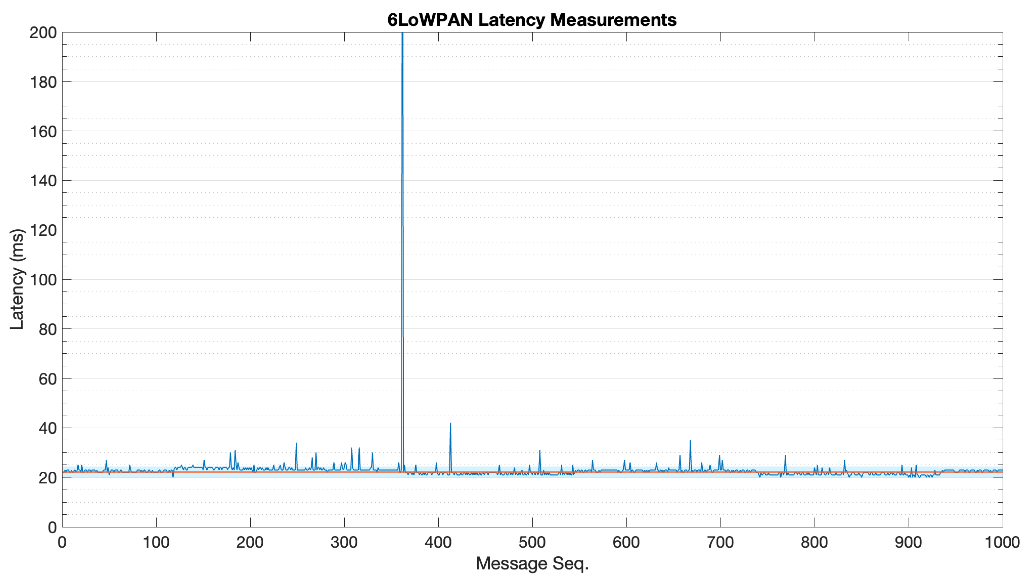
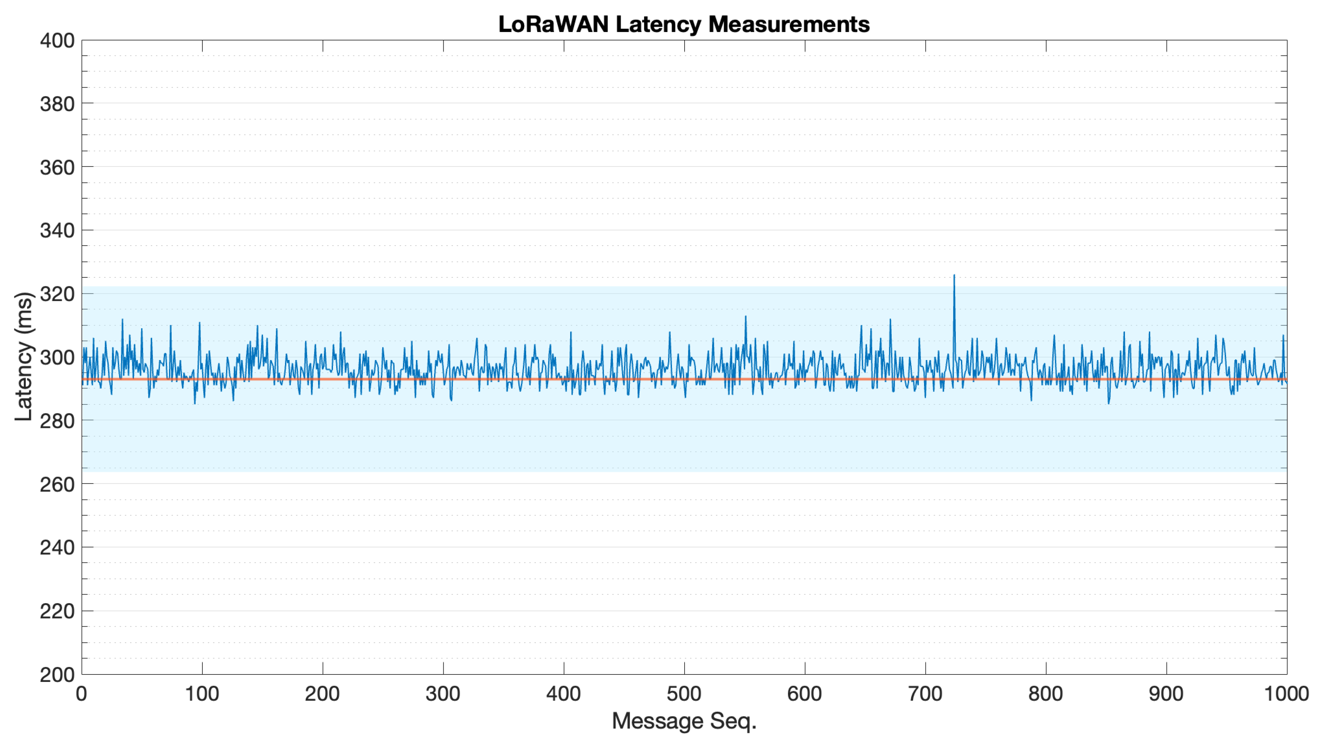
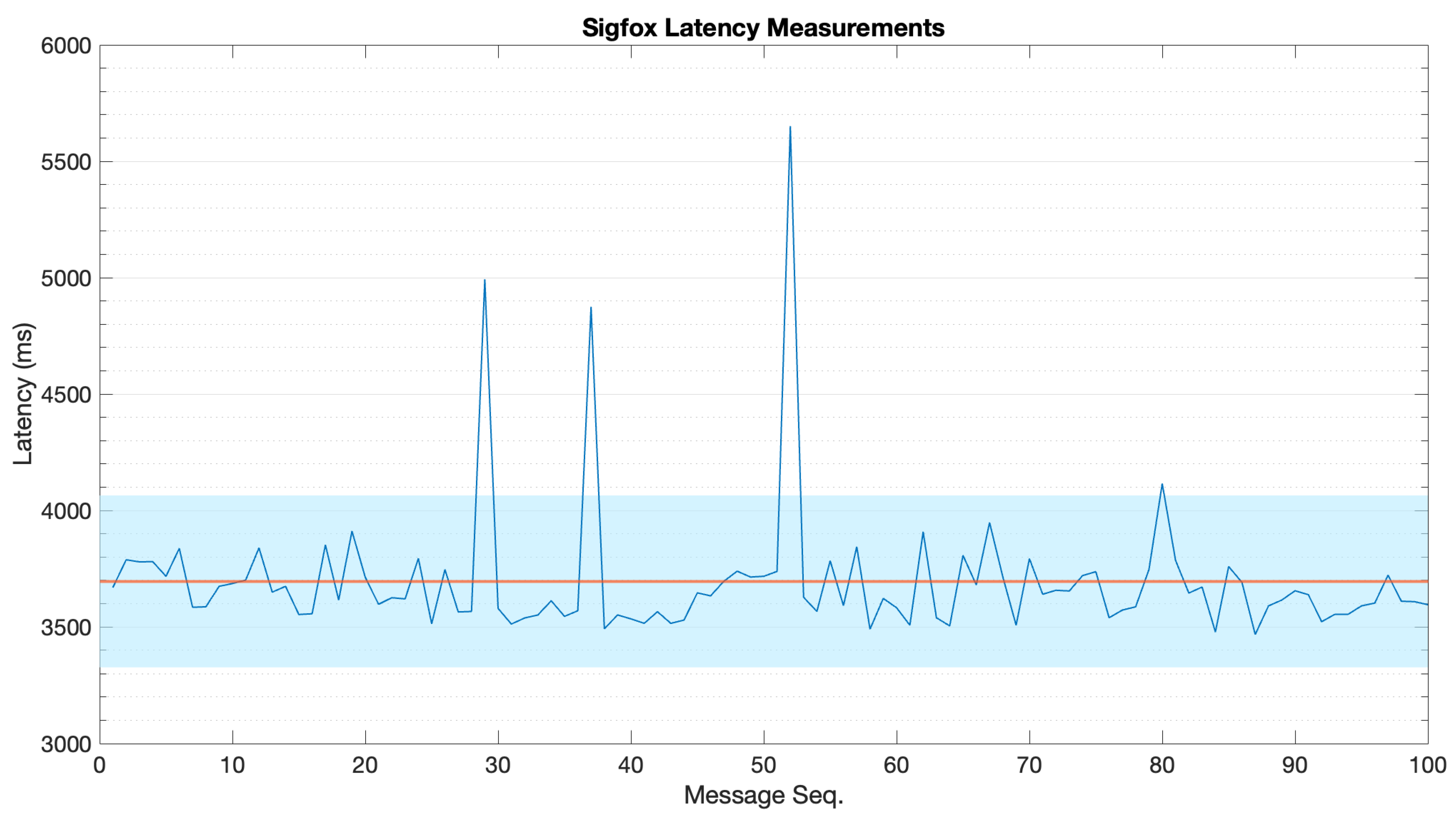
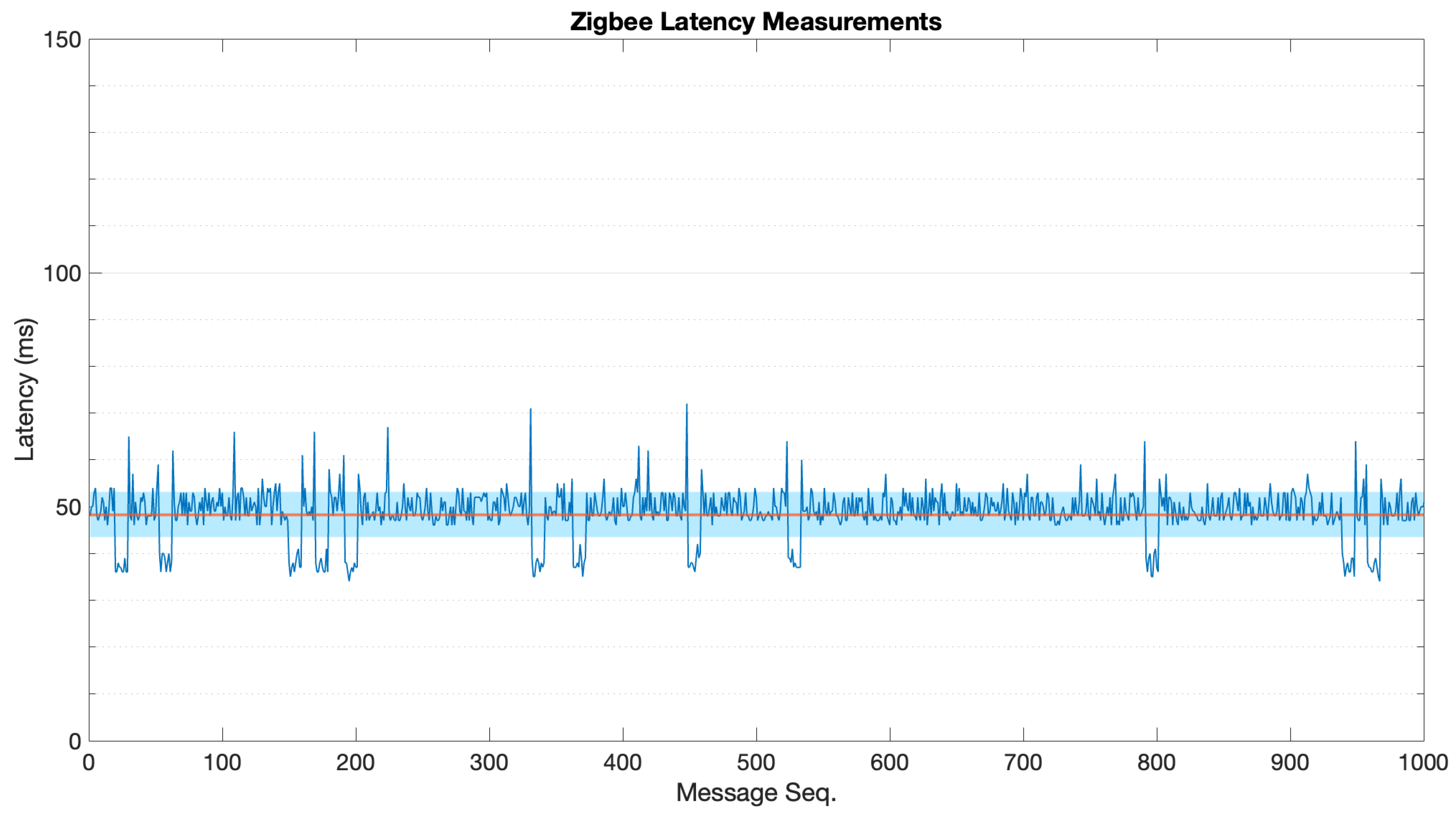
| Latency (ms) | Min. | 19.522 | 282.40 | 3467.1 | 34.174 | 25.294 | 13.382 | 329.29 |
| Avg. | 22.116 | 296.96 | 3695.2 | 48.298 | 32.300 | 26.974 | 1797.3 | |
| Max. | 356.14 | 334.81 | 5651.0 | 95.295 | 178.10 | 125.40 | 10,275 | |
| Error | 2 | 66 | 0 | 0 | 0 | 0 | 0 | |
| 0.02% | 0.66% | 0% | 0% | 0% | 0% | 0% | ||
| Stability | (ms) | 9.883 | 5.419 | 290.4 | 5.242 | 9.502 | 13.68 | 1352 |
| 386 | 2 | 4 | 2307 | 3197 | 480 | 4052 | ||
| 3.86% | 0.02% | 4% | 23.1% | 31.9% | 96.0% | 81.0% | ||
| 0.924 | 0.993 | 0.922 | 0.592 | 0.463 | 0.002 | 0.036 | ||
Publisher’s Note: MDPI stays neutral with regard to jurisdictional claims in published maps and institutional affiliations. |
© 2022 by the authors. Licensee MDPI, Basel, Switzerland. This article is an open access article distributed under the terms and conditions of the Creative Commons Attribution (CC BY) license (https://creativecommons.org/licenses/by/4.0/).
Share and Cite
Saavedra, E.; Mascaraque, L.; Calderon, G.; del Campo, G.; Santamaria, A. A Universal Testbed for IoT Wireless Technologies: Abstracting Latency, Error Rate and Stability from the IoT Protocol and Hardware Platform. Sensors 2022, 22, 4159. https://doi.org/10.3390/s22114159
Saavedra E, Mascaraque L, Calderon G, del Campo G, Santamaria A. A Universal Testbed for IoT Wireless Technologies: Abstracting Latency, Error Rate and Stability from the IoT Protocol and Hardware Platform. Sensors. 2022; 22(11):4159. https://doi.org/10.3390/s22114159
Chicago/Turabian StyleSaavedra, Edgar, Laura Mascaraque, Gonzalo Calderon, Guillermo del Campo, and Asuncion Santamaria. 2022. "A Universal Testbed for IoT Wireless Technologies: Abstracting Latency, Error Rate and Stability from the IoT Protocol and Hardware Platform" Sensors 22, no. 11: 4159. https://doi.org/10.3390/s22114159
APA StyleSaavedra, E., Mascaraque, L., Calderon, G., del Campo, G., & Santamaria, A. (2022). A Universal Testbed for IoT Wireless Technologies: Abstracting Latency, Error Rate and Stability from the IoT Protocol and Hardware Platform. Sensors, 22(11), 4159. https://doi.org/10.3390/s22114159