Abstract
Recently, a lot of attention has been paid to the field of research connected with the wireless sensor network and industrial internet of things. The solutions found by theorists are next used in practice in such area as smart industries, smart devices, smart home, smart transportation and the like. Therefore, there is a need to look for some new techniques for solving the problems described by means of the appropriate equations, including differential equations, integral equations and integro-differential equations. The object of interests of this paper is the method dedicated for solving some integro-differential equations with a retarded (delayed) argument. The proposed procedure is based on the Taylor differential transformation which enables to transform the given integro-differential equation into a respective system of algebraic (nonlinear, very often) equations. The described method is efficient and relatively simple to use, however a high degree of generality and complexity of problems, defined by means of the discussed equations, makes impossible to obtain a general form of their solution and enforces an individual approach to each equation, which, however, does not diminish the benefits associated with its use.
1. Introduction
In recent times, a dynamically developing field of research is the wireless sensor network and industrial internet of things. Theoretical solutions connected with these topics are next used in practical applications, in such area as smart industries, smart devices, smart home, smart transportation and the like. Therefore, there is a necessity to search for some new techniques for solving the problems described by means of appropriate equations, including differential equations, integral equations and integro-differential equations, in particular with a retarded argument.
Differential equations and integral equations with a retarded argument can find an application in many areas of science, among others, in mechanics, biophysics and control theory [1,2,3,4]. The integro-differential equation with a retarded argument in its full general form is not easy to find in mathematical models expressing the real existing processes, but some specific cases of this equations can be used in description of phenomena with viscoelastic effects [5,6], in the population dynamics, for example in the description of predator-prey models [7], as well as in modeling the problems connected with wireless sensor network and internet of things [8]. Analyzing the subject literature it is quite difficult to find any practical papers concerning the integral and integro-differential equations. The Taylor differential transformation, thanks to its properties, very often simplifies significantly the investigated problem, therefore it has a number of applications in mathematics, engineering and technics. Authors of this paper applied the Taylor differential transformation for solving, among others, the nonlinear ordinary differential equations, variational problems, systems of nonlinear ordinary differential equations, integro-differential equations, Stefan problem, as well as the integral equations [9,10,11]. The discussed transformation is also used by many authors for solving various problems, for example numerous kinds of differential equations (ordinary and partial) and integral equations, there exist also few well known papers devoted to the differential equations with a retarded argument [1,12,13,14,15,16,17,18]. The Taylor differential transformation is popular for a long time, but only recently the methods based on this transformation became useful due to the development of computers and programs enabling to execute the symbolic calculations, for example, in [19] the Authors apply the differential transform method to find the analytic solution to some delay differential equations with the help of the computer algebra system Mathematica, whereas in [20] DTM is compared with the other iterative method: the Daftardar-Gejji and Jafari Method in solving the differential equations. In this paper we also apply the Mathematica software in version 12.2 [21,22].
In this paper we discuss the integral differential equations with the delayed, or retarded, argument of the following form
with conditions
where , , , , , , whereas the functions f, , , , , are continuous in set . Similarly , , .
In Equation (1) the functions f, g and h can be nonlinear, whereas the integrals, occurring in this equation, can take the particular forms of integrals appearing in the Fredholm and Volterra integral equations, or they can have such form only with respect to the boundaries of integration, while the integrands and can be nonlinear also with respect to the sought function .
Equation (1) will be solved with the aid of the Taylor differential transformation, which, due to its properties, transforms this equation to the respective system of algebraic (nonlinear, very often) equations. The unknown elements in this systems are the coefficients of the Taylor series expanding the sought function. After solving the developed system of equations the approximate solution of the investigated equation can be determined.
Equation (1) in its full form appears rather rarely in the mathematical models describing some physical phenomena. One can find however the specific cases of this equation in the description of phenomena with viscoelastic effects. First papers concerning this problem were developed in the 20th century (by Boltzmann, Maxwell and Kelvin) and were devoted to investigating the creep and recovery phenomena in various materials. This theory evolved in the 20th century thanks to the research on polymers and this development continues even today. For example, paper [5] includes many models describing the viscoelasticity phenomenon, whereas in paper [6] one can find the Laederman model describing the reaction of the fibers creep to the predetermined tensions. This connection is expressed by the relation
where denotes the deformation, means the initial creep compliance, J is the creep compliance, denotes the tension, and is the tension function.
Particular cases of Equation (1) can be also found in the population dynamics, for example in the predator-prey model, described at first by Volterra [7] with the aid of the following system of equations (a similar issue was considered e.g., in work [23])
where and denote the number of predator and prey populations, respectively.
Model (3), modified by Brelot in [24], takes the form
where denotes the growth rate of the prey population under the assumption of the predators absence, is the self-regulation constant of the prey population, describes the predation of the prey by predators, denotes the death rate of predators under the assumption of the prey absence, is the conversion rate of predators, describes the intraspecies competition between the predators, functions F and G are the retardation functions responsible for including the prey and predators history into the model. Specific case of the equation System (4) is solved in Example 5.
Goal of this elaboration is to discuss the specific cases of the integro-differential equations with a retarded argument solved by using the new approach. Deriving the solution formula for the general form of the equation under consideration is impossible, but the discussed examples explain the way how to deal with these problems.
Novelty of this paper is a new approach to the solution of the equation in general form (1), based on the Taylor differential transformation. Contribution of the presented research is the development of an efficient technique for the solution of integro-differential equations with a retarded (delayed) argument with the use of the Taylor differential transformation and showing that the presented solution technique is efficient and relatively simple to use.
In Section 1 we introduce the equations being the object of our interests. Section 2 includes the theoretical description of the Taylor transformation together with its properties, particularly useful in the introduced solution procedure. Some of the properties are proved by example. In Section 3 we explain the details of the solution method and finally in Section 4 we illustrate the theoretical description with five example. The Section 5 contains some comments and conclusions.
2. The Taylor Transformation
Let us assume that we consider only such functions of the real variable x, defined in some region , which can be expanded into the Taylor series within some neighborhood of point . We call such functions as the originals and denote by the small letters of Latin alphabet, for example f, y, u, v, w, and so on. Thus, if the function y is the original, then the following equality holds
where is the point, in the neighborhood of which the function y is expanded into the Taylor series. Each original is assigned to a function of nonnegative integer arguments , according to formula
The function is called the image of the function y, the –function of the function y or the transform of the function y, and the discussed transformation is called the Taylor transformation.
The obvious fact is that, by having the –function one can find, according to Formulas (5) and (6), the corresponding original in the form of its expansion into the Taylor series, that is
Transformation (6), assigning to each original its image, is called the direct transformation. Whereas the transformation (7), assigning the corresponding original to the image, is called the inverse transformation. Connection between these both transformations will be denoted by means of the following symbols:
for the direct transformation and
for the inverse transformation, where and are the symbols of the proper transformations.
In the used notation, for example for the function and we have
where Whereas in case of the inverse transformation for the above function we get
The Taylor transformation possesses a number of properties causing that the application of this tool, with the aid of computational platforms giving the possibility to execute the symbolic calculations, like Mathematica for example, is quite simple.
In the current elaboration we use the specific case of the Taylor series—the Maclaurin series, therefore , constantly equal to zero, will be omitted henceforward.
Particularly, the following properties are very useful [1,13,14,25,26]:
Besides the “classic” Properties (8)–(14), the Taylor differential transformation possesses a number of properties corresponding to the retarded argument. Some of them are presented below (derivation of these formulas can be found, among others in [1], whereas some of these formulas, like for example Formula (33), are developed by the Authors):
, , , where .
As an example we prove the correctness of Formula (33). For this purpose we prove at first some auxiliary identities (in all these theorems we assume that the occurring functions are the originals).
Lemma 1
Proof.
Using the expansion of function y into the Taylor (Maclaurin) series, we have
hence we get the thesis
□
Lemma 2
Proof.
Using the expansion of function y into the Taylor series, we have
hence we get
□
Lemma 3.
If , , then
Proof.
Let , , then we have
where , , are unknown. Since the Relation (34) implies that , therefore we have
and by comparing the coefficients associated to the respective powers of x, we obtain successively
hence we get
Since for the last sum is “empty”, so it can be considered that the obtained formula holds true for all integers . Thus we have
which is the thesis of the lemma. □
Theorem 1
Proof.
Applying Lemmas 2 and 3 we can write that if , , then
where is the T-function of function , that is (see Lemma 2):
Thus we have
Now, by applying Lemma 1 we have , hence we get and for we have
On should pay a special attention to the sum of elements . We cannot simply substitute there the expression in place of k, because the coefficients F occur in this sum. Referring to the indices changed in this way we came across the negative indices. Such indices suppose to be properly retarded and the changed value, resulting from this retardation, must be regulated with the aid of appropriate multipliers. Hence we finally get for :
which ends the proof of theorem. □
3. Method of Solution
Besides the properties, listed above, for solving the equations of considered kind we will also use the initial Conditions (2). To use them efficiently, one should notice that
or else
hence, if we take , we get
Let us observe that in Formula (27), and in the similar formulas as well, the lower limit of integration is equal to the point, around which the given function is expanded into the Taylor series. According to the agreement, mentioned before, in this paper we take . If the case arises that in Equation (1) the lower limit of the Volterra type integral will be different than zero, then it is enough to notice, that if (independently whether , , or ):
where
and
then
4. Examples
Example 1.
We consider the equation
with condition
the exact solution of which is given by function .
Equation (37), under assumption and after applying, among others, the Properties (8), (11), (12), (13), (14), (24) and (26), transforms to the form
with the following equation included, on the grounds of initial Condition (38) and Formula (35):
Taking , Equation (39) leads to a system of equations of the form
Solving the system of Equations (41), we get three groups of solutions. After the appropriate verification (we assess the quality of the obtained approximate solution by substituting it into Equation (37)), it turns out that the best solution is , , , and , that is the function , which is the exact solution. For we obtain the same values , , and , , that is the same exact solution. It is worth noting that we did not need to use here the definition of .
Example 2.
We consider the equation
for , with conditions
the exact solution of which is given by function .
Equation (42), in result of applying, among others, the Properties (8), (10)–(12), (22)–(26) and (28), and using the initial Condition (43) (), develops into the form
with the following equation included, basing on the initial Condition (43) and Formula (35):
The unknowns of this system are , . Taking in Relations (44)–(45) we get the system of equations, the solution if which are , , , , , which gives
whereas by taking we obtain the approximate solution
Plots of the received solutions, together with the plots of absolute errors of these solutions
are presented in Figure 1, Figure 2, Figure 3 and Figure 4. In Figure 1 and Figure 3 the solid green line represents the exact solution, whereas the dashed red line marks the approximate solution. The errors are displayed in Figure 2 and Figure 4.
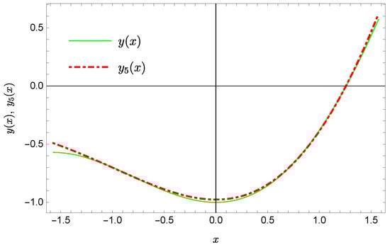
Figure 1.
Exact solution and the approximate solution .
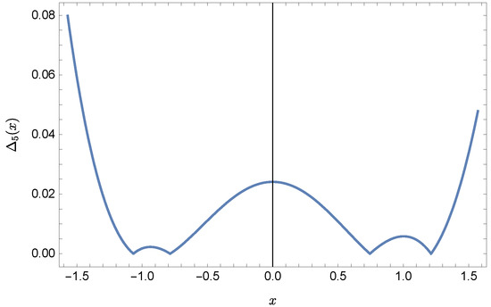
Figure 2.
Error of approximation .
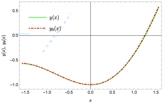
Figure 3.
Exact solution and the approximate solution .
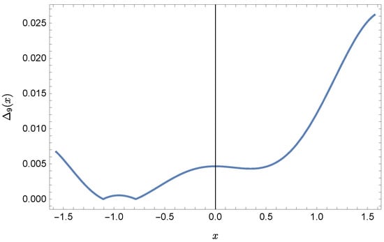
Figure 4.
Error of approximation .
Example 3.
Let us consider the equation
for , with conditions
the exact solution of which is defined by function .
Equation (46), under assumption
and after applying the Property (36), as well as under assumption
and after applying, among others, the Properties (8), (9), (11), (12), (13), (25) and (27), transforms into the form
where basing on Condition (47), with the following equation included, on the grounds of initial Condition (47) and Formula (35):
and the definitions of constants and given below
Taking the fixed value of N in Equations (48)–(50) we get the system of equations with unknowns , . So, taking , we receive in result the following approximate solution
with and (their exact values are , ). Whereas for we obtain the following approximate solution
with and .
Plots of the approximate Solutions (51) and (52), the exact solution and the absolute errors of these approximations are displayed in Figure 5, Figure 6, Figure 7 and Figure 8 (the notation of figures is the same as previously).
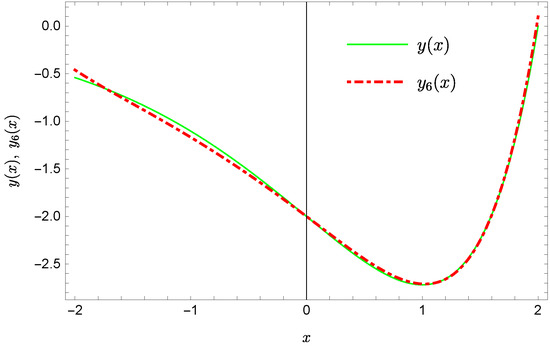
Figure 5.
Exact solution and the approximate solution .
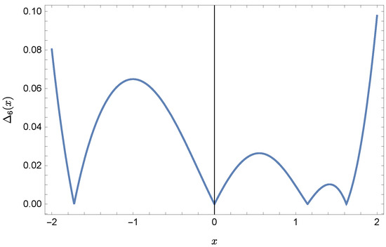
Figure 6.
Error of approximation .
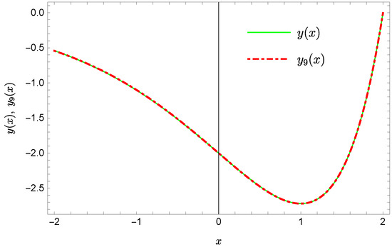
Figure 7.
Exact solution and the approximate solution .
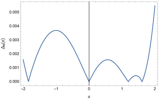
Figure 8.
Error of approximation .
Example 4.
Now we take into consideration the following equation
for , with conditions
the exact solution of which is described by function .
Equation (53), in result of applying the Property (36), that is assuming that
and in result of using, among others, the Properties (8), (9), (11), (12), (23), (24) and (33), develops into the form
where
where , basing on Condition (54), with the following definition of constant included
Assuming in (55) and (56) the fixed value of N we get the system of equations with unknowns , . So, value leads to the approximate solution
with (the exact value is ). Whereas for we obtain the approximate solution of the form
with .
Plots of the approximate Solutions (57) and (58), the exact solution and the absolute errors of these approximations are displayed in Figure 9, Figure 10, Figure 11 and Figure 12 (the previous notation of figures is kept).
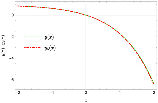
Figure 9.
Exact solution and the approximate solution .
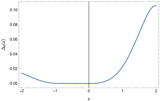
Figure 10.
Error of approximation .
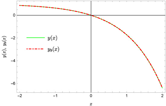
Figure 11.
Exact solution and the approximate solution .
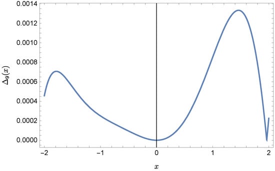
Figure 12.
Error of approximation .
Example 5.
Let us solve the specific case of the system of Equation (4), in which we take: , , , , . Then the system takes the form
for , with conditions
the exact solution of which is given by functions and .
System of Equations (59), after applying the properties of the Taylor transformation (see (16) where ), can be written in the following form
Using the Conditions (60) and taking in Relations (61) the successive values , we get in turn
- —
- for :
- —
- for : hence we get
- —
- for : hence we get
- —
- for : hence we get
Limiting the k values to we get the approximate solution
Since function z is reconstructed exactly, Figure 13 presents only the comparison of the exact solution y and the approximate solution (the notation of figures is the same as in the previous examples) together with the graph of absolute error of this approximation. Next, Figure 14 shows the corresponding graphs for the approximate solution .
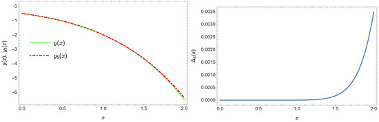
Figure 13.
Exact solution and the approximate solution together with the error of this approximation.
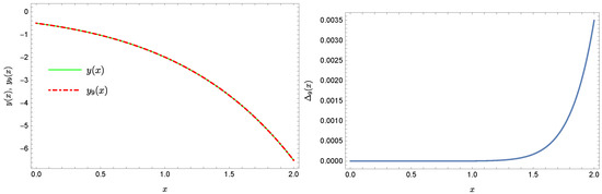
Figure 14.
Exact solution and the approximate solution together with the error of this approximation.
Interesting is that we obtain in the successive steps the exact values of coefficients of the expansions of functions and into the Taylor series, which means that if only we would be able to discover this relation, we could obtain the exact solution of System (5).
5. Conclusions
This paper discusses the possibility of applying the Taylor differential transformation for solving the integro-differential equations with a retarded argument. The investigated equations are important, because we can find them in various mathematical, technical and engineering problems, and simultaneously, solving them is not an easy task. So, the contribution of the presented research is the development of an efficient technique for the solution of nonlinear equations which may arise in the area of up-growing interest, like the wireless sensor network and industrial internet of things. Examples, presented in this elaboration, show that the solution technique based on the Taylor differential transformation is efficient in case of equations of considered kind and its additional advantage is the simplicity of its application. The discussed method is well applicable when the sought function is expandable into the Taylor series in the considered region. In all cases, examined in the current paper and elsewhere, the satisfactory solution was possible to find always when this assumption was satisfied. In future we plan to compare the discussed method with some similar methods based on other transformations, like, for example, the Laplace transform. Moreover, we plan to apply DTM for solving some problems described by the equations with fractional derivative.
Author Contributions
All authors contributed equally to the research. All authors have read and agreed to the published version of the manuscript.
Funding
This research received no external funding.
Institutional Review Board Statement
Not applicable.
Informed Consent Statement
Not applicable.
Data Availability Statement
Not applicable.
Conflicts of Interest
The author declare no conflict of interest. The funders had no role in the design of the study; in the collection, analyses, or interpretation of data; in the writing of the manuscript, or in the decision to publish the results.
References
- Arikoglu, A.; Ozkol, I. Solution of differential-difference equations by using differential transform method. Appl. Math. Comput. 2006, 174, 153–162. [Google Scholar] [CrossRef]
- Elmer, C.E.; van Vleck, E.S. A Variant of Newton’s Method for the Computation of Traveling Waves of Bistable Differential-Difference Equations. J. Dyn. Differ. Equat. 2002, 14, 493–517. [Google Scholar] [CrossRef]
- Rodríguez, F.; López, J.C.C.; Castro, M.A. Models of Delay Differential Equations; MDPI: Basel, Switzerland, 2021. [Google Scholar]
- Smith, H. An Introduction to Delay Differential Equations with Applications to the Life Sciences; Springer: New York, NY, USA, 2011. [Google Scholar]
- Drozdov, A.D. Finite Elasticity and Viscoelasticity. A Course in the Nonlinear Mechanics of Solids; World Scientific Publishing: Singapore, 1996. [Google Scholar]
- Smart, J.; Aruna, K.; Williams, J. A comparison of single-integral non-linear viscoelasticity theories. J. Mech. Phys. Solids 1972, 20, 313–324. [Google Scholar] [CrossRef]
- Volterra, V. Sur la théorie mathématique des phénomènes héréditaires. J. Mathématiques Pures Appliquées 1928, 7, 249–298. [Google Scholar]
- Amin, R.; Nazir, S.; García-Magariño, I. A Collocation Method for Numerical Solution of Nonlinear Delay Integro-Differential Equations for Wireless Sensor Network and Internet of Things. Sensors 2020, 20, 1962. [Google Scholar] [CrossRef] [PubMed]
- Grzymkowski, R.; Hetmaniok, E.; Pleszczyński, M. A novel algorithm for solving the ordinary differential equations. In Selected Problems on Experimental Mathematics; Hetmaniok, E., Słota, D., Trawiński, T., Wituła, R., Eds.; Silesian University of Technology Press: Gliwice, Poland, 2017; pp. 103–112. [Google Scholar]
- Grzymkowski, R.; Pleszczyński, M. Application of the Taylor transformation to the systems of ordinary differential equations. In Proceedings of the Information and Software Technologies, ICIST 2018, Communications in Computer and Information Science, Vilnius, Lithuania, 4–6 October 2018; Damasevicius, R., Vasiljeviene, G., Eds.; Springer: Cham, Switzerland, 2018. [Google Scholar]
- Hetmaniok, E.; Pleszczyński, M. Comparison of the Selected Methods Used for Solving the Ordinary Differential Equations and Their Systems. Mathematics 2022, 10, 306. [Google Scholar] [CrossRef]
- Biazar, J.; Eslami, M.; Islam, M.R. Differential transform method for special systems of integral equations. J. King Saud Univ. Sci. 2012, 24, 211–214. [Google Scholar] [CrossRef]
- Doğan, N.; Ertürk, V.S.; Momani, S.; Akın, Ö.; Yıldırım, A. Differential transform method for solving singularly perturbed Volterra integral equations. J. King Saud Univ. Sci. 2011, 23, 223–228. [Google Scholar] [CrossRef]
- Odibat, Z.M. Differential transform method for solving Volterra integral equation with separable kernels. Math. Comput. Model. 2008, 48, 1144–1149. [Google Scholar] [CrossRef]
- Ravi Kanth, A.S.V.; Aruna, K. Differential transform method for solving the linear and nonlinear Klein–Gordon equation. Comput. Phys. Commun. 2009, 185, 708–711. [Google Scholar] [CrossRef]
- Ravi Kanth, A.S.V.; Aruna, K.; Chaurasial, R.K. Reduced differential transform method to solve two and three dimensional second order hyperbolic telegraph equations. J. King Saud Univ. Eng. Sci. 2017, 29, 166–171. [Google Scholar]
- Srivastava, V.K.; Awasthi, M.K. Differential transform method for solving linear and non-linear systems of partial differential equations. Phys. Lett. A 2008, 372, 6896–6898. [Google Scholar]
- Tari, A.; Shahmorad, S. Differential transform method for the system of two-dimensional nonlinear Volterra integro-differential equations. Comput. Math. Appl. 2011, 61, 2621–2629. [Google Scholar] [CrossRef][Green Version]
- Liu, B.Q.; Zhou, X.J.; Du, Q.K. Differential Transform Method for Some Delay Differential Equations. Appl. Math. 2015, 6, 585–593. [Google Scholar] [CrossRef][Green Version]
- Sharma, V.S.; Joshi, M.A. A Comparison Between Two Approaches to Solve Functional Differential Equations: DTM and DJM. Int. J. Math. Appl. 2017, 5, 521–527. [Google Scholar]
- Wolfram, S. An Elementary Introduction to the Wolfram Language, 2nd ed.; Wolfram Media, Inc.: Champaign, IL, USA, 2017. [Google Scholar]
- Wolfram, S. The Mathematica Book, 5th ed.; Wolfram Media, Inc.: Champaign, IL, USA, 2003. [Google Scholar]
- Tari, A. The Differential Transform Method for solving the model describing biological species living together. Iran. J. Math. Sci. Inform. 2012, 7, 63–74. [Google Scholar]
- Brelot, M. Sur le problème biologique héréditaiare de deux especès dévorante et dévorée. Ann. Mat. Pura Appl. 1931, 9, 58–74. [Google Scholar] [CrossRef]
- Arikoglu, A.; Ozkol, I. Solution of boundary value problems for integro-differential equations by using differential transform method. Appl. Math. Comput. 2005, 168, 1145–1158. [Google Scholar] [CrossRef]
- Arikoglu, A.; Ozkol, I. Solutions of integral and integro-differential equation systems by using differential transform method. Comput. Math. Appl. 2008, 56, 2411–2417. [Google Scholar] [CrossRef][Green Version]
Publisher’s Note: MDPI stays neutral with regard to jurisdictional claims in published maps and institutional affiliations. |
© 2022 by the authors. Licensee MDPI, Basel, Switzerland. This article is an open access article distributed under the terms and conditions of the Creative Commons Attribution (CC BY) license (https://creativecommons.org/licenses/by/4.0/).