
Establishing A Sustainable Low-Cost Air Quality Monitoring Setup: A Survey of the State-of-the-Art


Abstract
:1. Introduction
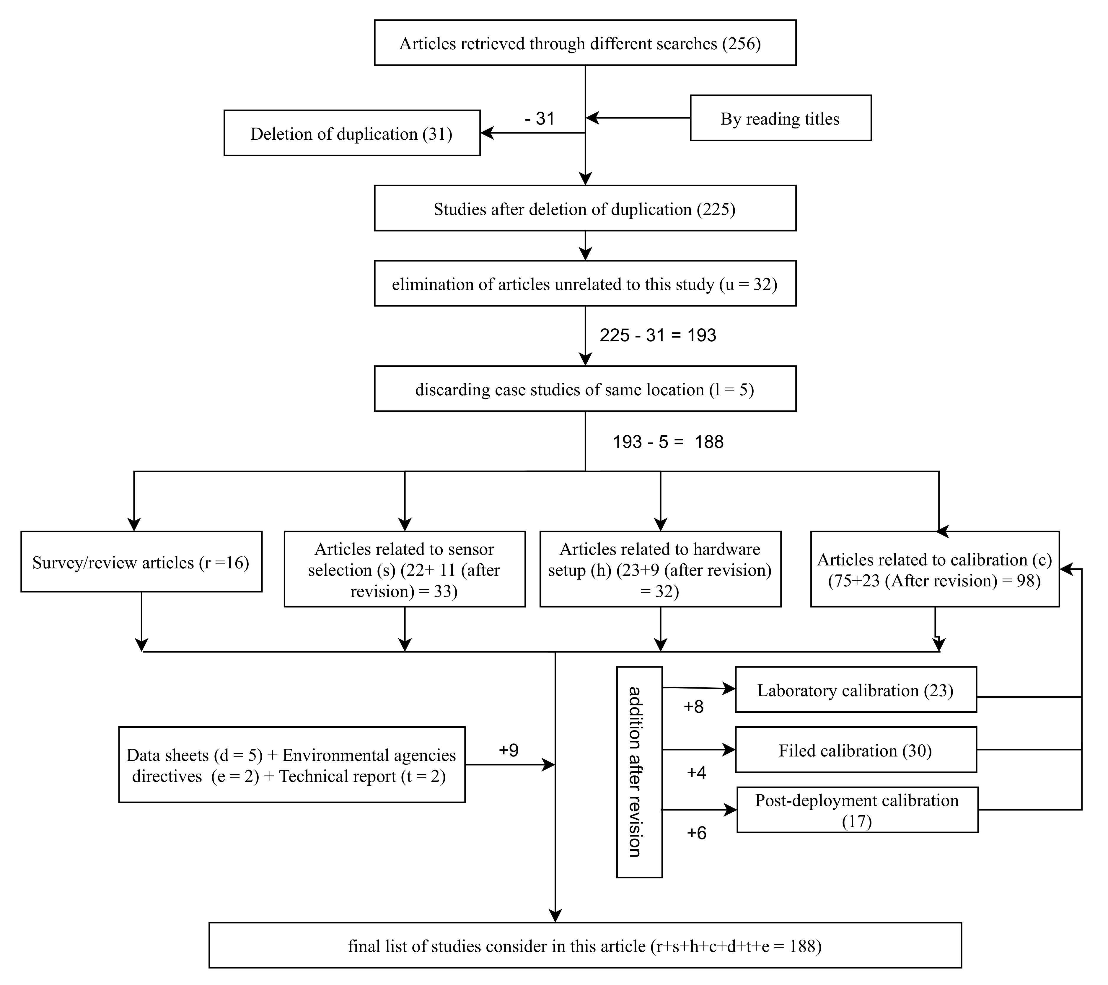
1.1. Literature Review
1.2. Our Contribution
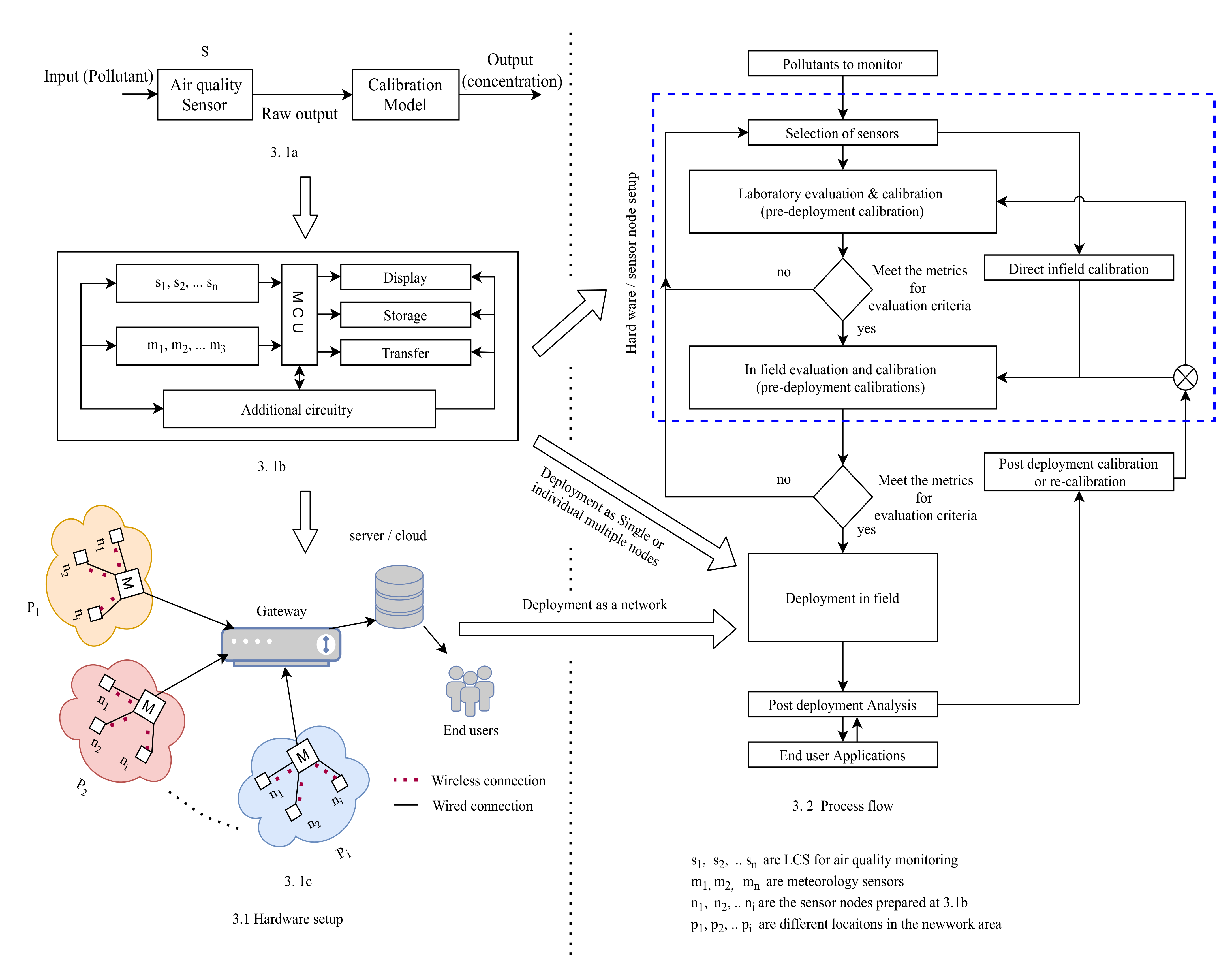
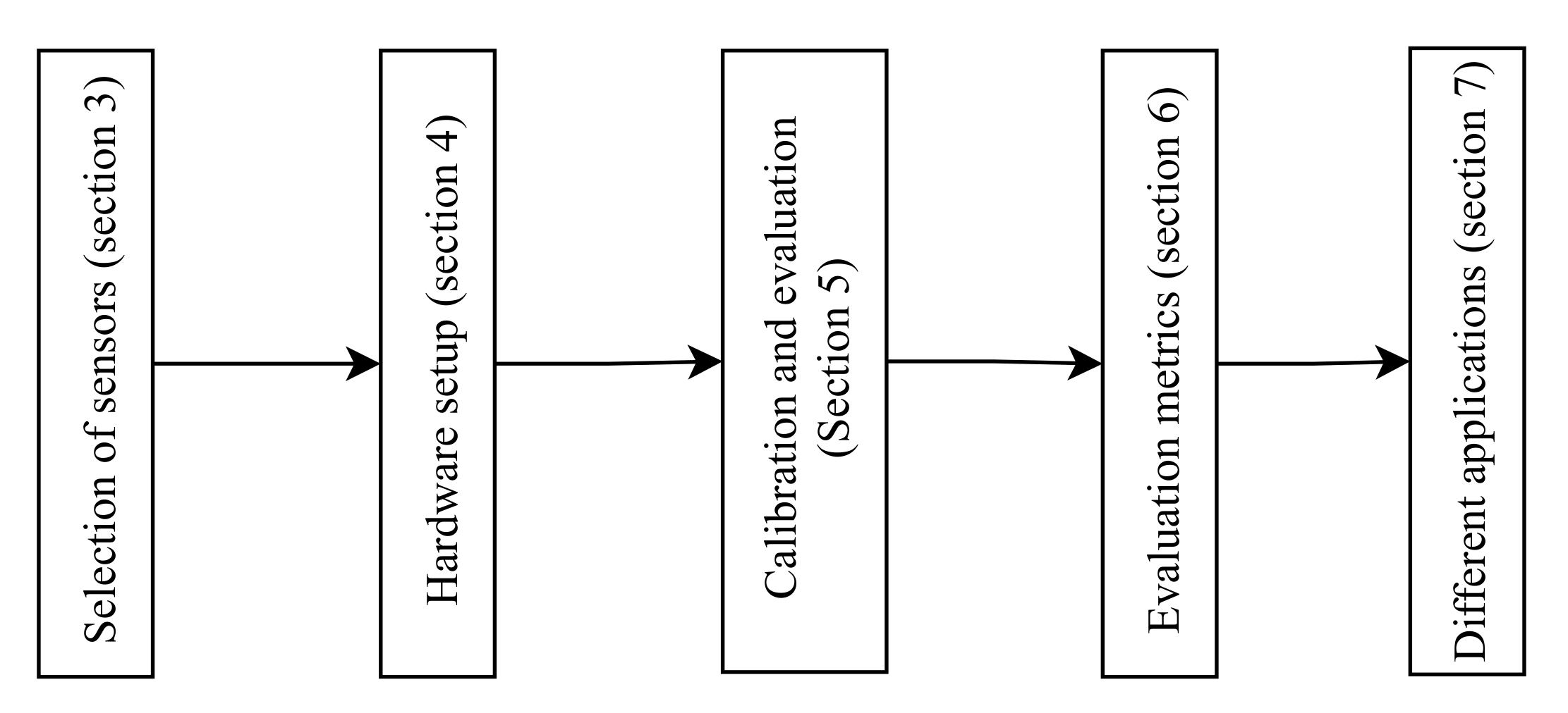
2. LCS Based Air Pollution Measurement
- Step 1:
- Select appropriate sensors for the given set of conditions and applications (Section 3).
- Step 2:
- Calibrate the selected sensors in a laboratory under controlled environmental conditions at different concentrations of pollutants (Section 5.1.1). Once the laboratory calibration is finished, check the performance of the sensors with different evaluation metrics (various evaluation metrics to test LCS are discussed in Section 6). If the performance (in terms of accuracy or precision) is not satisfactory, then repeat step 1, i.e., selection of sensors; otherwise, go to step 3.
- Step 3:
- Calibrate the sensors in the field and evaluate their performance (Section 5.1.2). Once the field test is completed, they are ready to deploy in real-time in the field.
- Step 4:
- Do frequent post-deployment analysis to check for data quality in real-time, which will help to identify the re-calibration requirement. In general, re-calibration is recommended to do at least once a month (Section 5.2).
3. Selection of Sensors
- Particulate matter sensors (PMS);
- GAS sensors (GS).
3.1. PMS
- Federal reference method (FRM): Gravimetric method is a FRM and it is a direct method to measure PM;
- Federal equivalent methods (FEM): Tapered element oscillating microbalance (TEOM), Beta Attenuation Monitor (BAM) are two different FEM methods to measure PM;
- Low-cost sensors: Most of the commercial particulate sensors are based on the light scattering principle, and few of them are work on other principles like digital holography and microscopy.
3.1.1. Light Scattering Method
- Less cost and portable;
- Easy to operate and able to integrate with IOT network;
- High data resolution.
- PMS based on the light scattering principle can be used for particles of a size greater than 0.3 μm because particles of a size less than 0.3 μm may not scatter sufficient light to get particle count [54];
- Drift in the response due to the degradation of the laser source;
- Temperate and humidity can effect the sensor performance.
3.1.2. Digital Holography Method
- Able to detect particles of size in the lower μm-range, which is not possible in the light scattering method;
- It is an image based system hence there is no need to consider the flow rate monitoring;
- Possibility to find the chemical composition of particles by using the size and colour properties in the images.
- The sampling rate is less than that of sensors based on light scattering method.
3.1.3. Microscopy Method
- High volume sampling;
- Can detect sub-micron sized particles;
- Possible to detect Chemical characteristics of PM.
- Expensive compared to light scattering sensors.
3.2. Gas Sensors (GS)
3.2.1. MOS Sensors
- They can work at higher temperatures and have a higher operational lifetime compared to EC sensors;
- High sensitivity;
- Less cost, portable and IoT integrable;
- High resolution data.
- Heating of metal oxide surface is the limitation in MOS sensors. Pre-heating requires high operational power that makes MOS expensive in terms of power consumption;
- Higher humidity levels can reduce the metal oxide surface’s sensitivity, making the MOS less accurate when compared with ECS at higher humidity levels;
- Drift in the sensor performance due to the sensitivity loss of metal oxide surface overtime.
3.2.2. EC Sensors
- ECS consume less power than MOS;
- High sensitivity;
- Less impacted by higher humidity values than the MOS sensors;
- Compact, portable and IoT integrable.
- Less operational time than ECS due to the degradation of electrolyte performance over time;
- ECS have a higher response time when compared to metal oxide sensors. In order to obtain the corresponding output to the applied input ECS undergo chemical reactions that cause the delay in response time.
3.2.3. NDIR Sensors
- Compact and requires less power;
- High operational life time.
- Higher cost compared to ECS and MOS;
- Presence of moisture content in the air sample can cause the spectral interference that leads to inaccurate measurement.
3.2.4. PID Sensors
- Low power requirements;
- High sensitivity and short response time.
- Very high cost;
- Difficult to design for a particular pollutant since UV light can ionize all the gases whose ionization potential is less than the energy of the UV light.
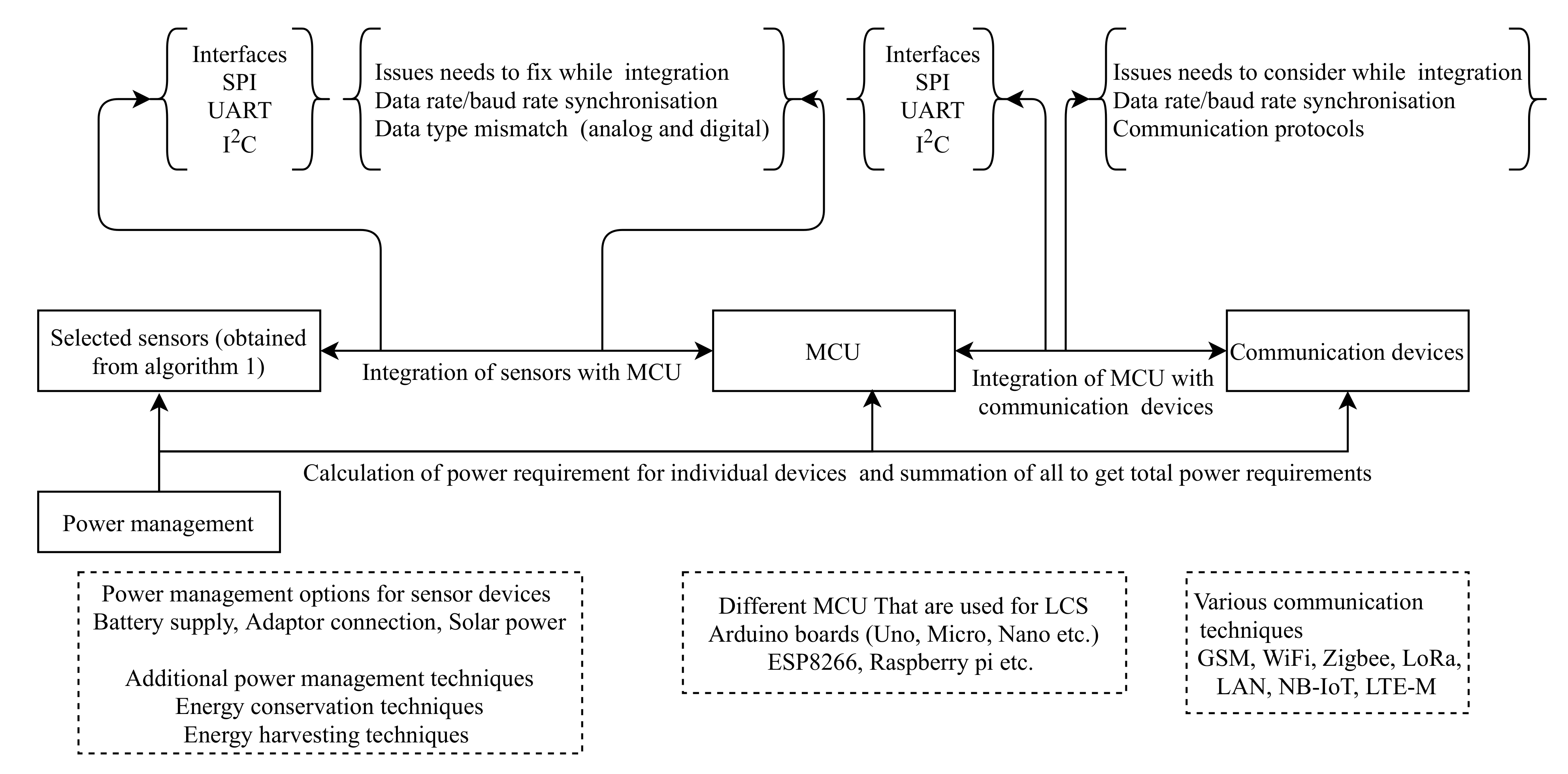
4. Hardware Setup/Sensor Node Design
- Integration of sensors with MCU;
- Integration of MCU with communication devices;
- Power management

4.1. Integration of Sensors with MCU
4.2. Power Management
4.3. Integration of Sensors with Communication Devices
- Sensors’ operational lifetime depends on the lifetime of internal components of the sensors. The lifetime that is least among the internal components of a sensor is the operational lifetime of that sensor. For example, an optical sensor’s lifetime depends on a light emitting source (laser source) and photo detector. Therefore the light emitting or photo diode which has the least operational lifetime is considered the operational lifetime of the optical sensor.
- LCS performance drifts overtime. Main reason for the sensor response drift is the degradation of sensing material or sensing mechanism. This drift can be clearly visible in the time series or trend lines. Therefore identification of unusual drifts in the sensor output signals the replacement of the sensor prior to the end of operational lifetime;
- Sensor output trend reversal when compared with reference instruments values and continuous outliers also helps to recognize the requirement of sensor replacement.
5. Calibration and Evaluation
5.1. Pre-Deployment Calibration and Evaluation
- 1.
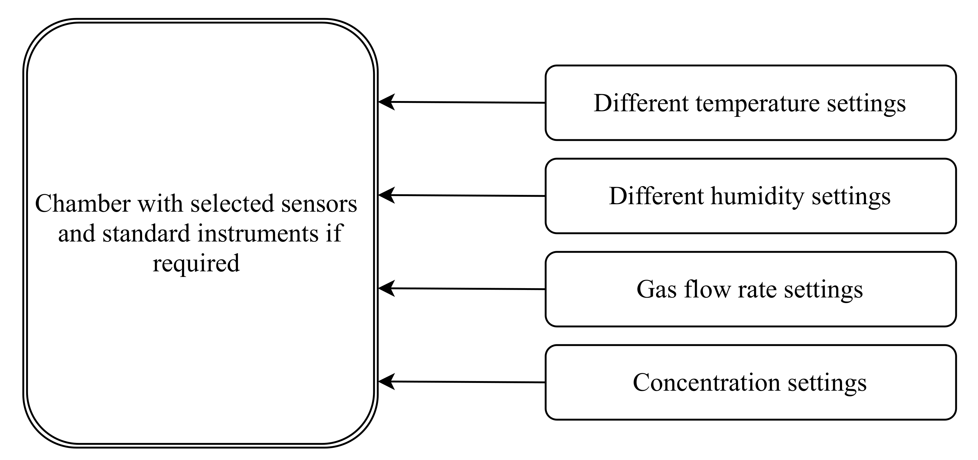
- At the laboratory with controlled environmental conditions by using standard gaseous mixtures;
- 2.
- In the field with uncontrolled real-time environmental effects.
5.1.1. Laboratory Calibration and Evaluation
5.1.2. In-Field Calibration and Validation
5.2. Post-Deployment Calibration and Evaluation
- 1.
- By replacing the calibration parameters in the sensor nodes. In order to do this, we need to incorporate the re-calibration mechanism within the sensor node, which requires high computational power. At the same time, it is not feasible to handle extensive data at the sensors node;
- 2.
- Doing calibration in the cloud by taking raw sensor data as the inputs. With this technique we can overcome the limitations in the former method.
6. Evaluation Metrics
6.1. Sensor vs. Reference
6.2. Sensor vs. Sensor
6.3. Model vs. Model
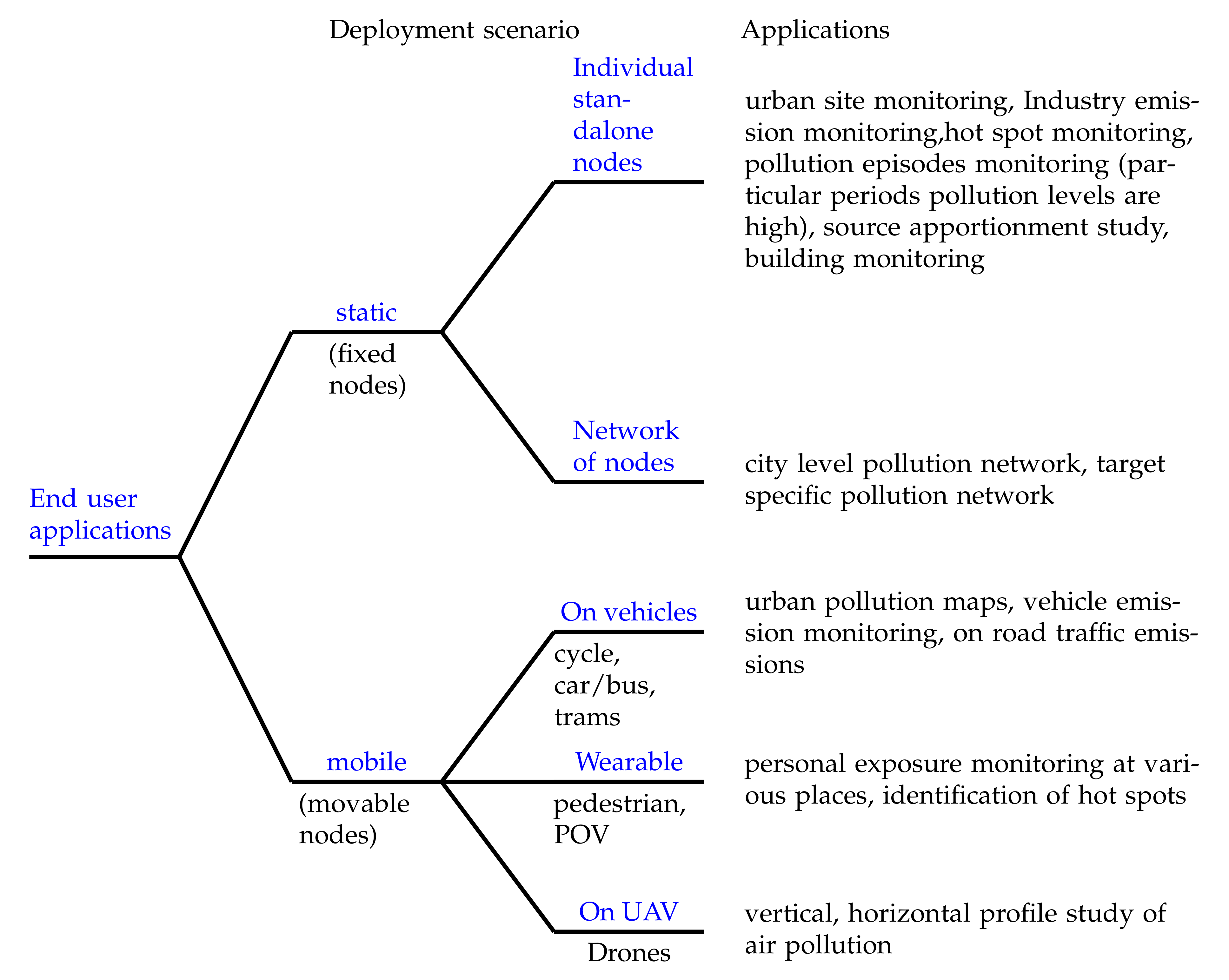
7. End User Applications
7.1. Static Deployment
7.2. Mobile Deployments
8. Conclusions and Future Scope
Supplementary Materials
Author Contributions
Funding
Institutional Review Board Statement
Informed Consent Statement
Data Availability Statement
Conflicts of Interest
References
- Barbera, E.; Currò, C.; Valenti, G. A hyperbolic model for the effects of urbanization on air pollution. Appl. Math. Model. 2010, 34, 2192–2202. [Google Scholar] [CrossRef] [Green Version]
- Kumar, P.; Khare, M.; Harrison, R.M.; Bloss, W.J.; Lewis, A.C.; Coe, H.; Morawska, L. New directions: Air pollution challenges for developing megacities like Delhi. Atmos. Environ. 2015, 122, 657–661. [Google Scholar] [CrossRef]
- Correia, A.W.; Arden Pope, C.; Dockery, D.W.; Wang, Y.; Ezzati, M.; Dominici, F. Effect of air pollution control on life expectancy in the United States: An analysis of 545 U.S. Counties for the period from 2000 to 2007. Epidemiology 2013, 24, 23–31. [Google Scholar] [CrossRef] [PubMed] [Green Version]
- Kampa, M.; Castanas, E. Human health effects of air pollution. Environ. Pollut. 2008, 151, 362–367. [Google Scholar] [CrossRef]
- Meister, K.; Johansson, C.; Forsberg, B. Estimated short-term effects of coarse particles on daily mortality in Stockholm, Sweden. Environ. Health Perspect. 2013, 120, 431–436. [Google Scholar] [CrossRef] [Green Version]
- Saini, P.; Sharma, M. Cause and Age-specific premature mortality attributable to PM2.5 Exposure: An analysis for Million-Plus Indian cities. Sci. Total Environ. 2020, 710, 135230. [Google Scholar] [CrossRef]
- Jacobson, M.Z. Review of solutions to global warming, air pollution, and energy security. Energy Environ. Sci. 2009, 2, 148–173. [Google Scholar] [CrossRef]
- Bergin, M.H.; Tripathi, S.N.; Jai Devi, J.; Gupta, T.; Mckenzie, M.; Rana, K.S.; Shafer, M.M.; Villalobos, A.M.; Schauer, J.J. The discoloration of the Taj Mahal due to particulate carbon and dust deposition. Environ. Sci. Technol. 2015, 49, 808–812. [Google Scholar] [CrossRef]
- Winner, W.E. Mechanistic Analysis of Plant Responses to Air Pollution. Ecol. Appl. 1994, 4, 651–661. [Google Scholar] [CrossRef]
- Gulia, S.; Shiva Nagendra, S.M.; Khare, M.; Khanna, I. Urban air quality management—A review. Atmos. Pollut. Res. 2015, 6, 286–304. [Google Scholar] [CrossRef] [Green Version]
- DownToEarth. India’s Air “Toxic”: WHO. Available online: https://www.downtoearth.org.in/news/air/indias-toxic-air-the-who-60377 (accessed on 21 April 2020).
- Guttikunda, S.K.; Goel, R.; Pant, P. Nature of air pollution, emission sources, and management in the Indian cities. Atmos. Environ. 2014, 95, 501–510. [Google Scholar] [CrossRef]
- Pandey, A.; Brauer, M.; Cropper, M.L.; Balakrishnan, K.; Mathur, P.; Dey, S.; Turkgulu, B.; Kumar, G.A.; Khare, M.; Beig, G.; et al. Health and economic impact of air pollution in the states of India: The Global Burden of Disease Study 2019. Lancet Planet. Health 2021, 5, e25–e38. [Google Scholar] [CrossRef]
- Menon, J.S.; Nagendra, S.M.S. Personal exposure to fine particulate matter concentrations in central business district of a tropical coastal city. J. Air Waste Manag. Assoc. 2018, 68, 415–429. [Google Scholar] [CrossRef] [Green Version]
- Nagendra, S.M.S.; Reddy Yasa, P.; Narayana, M.V.; Khadirnaikar, S.; Rani, P. Mobile monitoring of air pollution using low cost sensors to visualize spatio-temporal variation of pollutants at urban hotspots. Sustain. Cities Soc. 2019, 44, 520–535. [Google Scholar] [CrossRef]
- Piedrahita, R.; Xiang, Y.; Masson, N.; Ortega, J.; Collier, A.; Jiang, Y.; Li, K.; Dick, R.P.; Lv, Q.; Hannigan, M.; et al. The next generation of low-cost personal air quality sensors for quantitative exposure monitoring. Atmos. Meas. Tech. 2014, 7, 3325–3336. [Google Scholar] [CrossRef] [Green Version]
- Central Polluton Control Board (CPCB) Continuous Ambient Air Quality Monitoring Station (CAAQMS) List. Available online: https://app.cpcbccr.com/ccr/#/login (accessed on 2 June 2020).
- Morawska, L.; Thai, P.K.; Liu, X.; Asumadu-Sakyi, A.; Ayoko, G.; Bartonova, A.; Bedini, A.; Chai, F.; Christensen, B.; Dunbabin, M.; et al. Applications of low-cost sensing technologies for air quality monitoring and exposure assessment: How far have they gone? Environ. Int. 2018, 116, 286–299. [Google Scholar] [CrossRef]
- Chojer, H.; Branco, P.T.B.S.; Martins, F.G.; Alvim-Ferraz, M.C.M.; Sousa, S.I.V. Development of low-cost indoor air quality monitoring devices: Recent advancements. Sci. Total Environ. 2020, 727, 138385. [Google Scholar] [CrossRef]
- Zimmerman, N.; Presto, A.A.; Kumar, S.P.N.; Gu, J.; Hauryliuk, A.; Robinson, E.S.; Robinson, A.L.; Subramanian, R. A machine learning calibration model using random forests to improve sensor performance for lower-cost air quality monitoring. Atmos. Meas. Tech. 2018, 11, 291–313. [Google Scholar] [CrossRef] [Green Version]
- Becnel, T.; Tingey, K.; Whitaker, J.; Sayahi, T.; Le, K.; Goffin, P.; Butterfield, A. A Distributed Low-Cost Pollution Monitoring Platform. IEEE Internet Things J. 2019, 6, 10738–10748. [Google Scholar] [CrossRef]
- Sahu, R.; Dixit, K.K.; Mishra, S.; Kumar, P.; Shukla, A.K.; Sutaria, R.; Tiwari, S.; Tripathi, S.N. Validation of low-cost sensors in measuring real-time PM10 concentrations at two sites in delhi national capital region. Sensors 2020, 20, 1347. [Google Scholar] [CrossRef] [Green Version]
- Cross, E.S.; Lewis, D.K.; Williams, L.R.; Magoon, G.R.; Kaminsky, M.L.; Worsnop, D.R.; Jayne, J.T. Use of electrochemical sensors for measurement of air pollution: Correcting interference response and validating measurements. Atmos. Meas. Tech. Discuss. 2017, 10, 3575–3588. [Google Scholar] [CrossRef] [Green Version]
- Barcelo-Ordinas, J.M.; Ferrer-Cid, P.; Garcia-Vidal, J.; Ripoll, A.; Viana, M. Distributed multi-scale calibration of low-cost ozone sensors in wireless sensor networks. Sensors 2019, 19, 2503. [Google Scholar] [CrossRef] [Green Version]
- Hasenfratz, D.; Saukh, O.; Walser, C.; Hueglin, C.; Fierz, M.; Arn, T.; Beutel, J.; Thiele, L. Deriving high-resolution urban air pollution maps using mobile sensor nodes. Pervasive Mob. Comput. 2015, 16, 268–285. [Google Scholar] [CrossRef]
- Schneider, P.; Castell, N.; Vogt, M.; Dauge, F.R.; Lahoz, W.A.; Bartonova, A. Mapping urban air quality in near real-time using observations from low-cost sensors and model information. Environ. Int. 2017, 106, 234–247. [Google Scholar] [CrossRef]
- Moltchanov, S.; Levy, I.; Etzion, Y.; Lerner, U.; Broday, D.M.; Fishbain, B. On the feasibility of measuring urban air pollution by wireless distributed sensor networks. Sci. Total Environ. 2015, 502, 537–547. [Google Scholar] [CrossRef]
- Spinelle, L.; Gerboles, M.; Villani, M.G.; Aleixandre, M.; Bonavitacola, F. Field calibration of a cluster of low-cost commercially available sensors for air quality monitoring. Part B. Sens. Actuators B 2017, 238, 706–715. [Google Scholar] [CrossRef]
- Maag, B.; Saukh, O.; Hasenfratz, D.; Thiele, L. Pre-Deployment Testing, Augmentation and Calibration of Cross-Sensitive Sensors. In Proceedings of the International Conference EWSN ’16, Graz, Austria, 15–17 February 2016; pp. 169–180. [Google Scholar]
- Jayaratne, R.; Liu, X.; Thai, P.; Dunbabin, M.; Morawska, L. The influence of humidity on the performance of a low-cost air particle mass sensor and the effect of atmospheric fog. Atmos. Meas. Tech. 2018, 11, 4883–4890. [Google Scholar] [CrossRef] [Green Version]
- Samad, A.; Obando Nuñez, D.R.; Solis Castillo, G.C.; Laquai, B.; Vogt, U. Effect of Relative Humidity and Air Temperature on the Results Obtained from Low-Cost Gas Sensors for Ambient Air Quality Measurements. Sensors 2020, 20, 5175. [Google Scholar] [CrossRef]
- Bai, L.; Huang, L.; Wang, Z.; Ying, Q.; Zheng, J.; Shi, X.; Hu, J. Long-term Field Evaluation of Low-cost Particulate Matter Sensors in Nanjing. Aerosol Air Q. Res. 2020, 20, 242–253. [Google Scholar] [CrossRef]
- Rai, A.C.; Kumar, P.; Pilla, F.; Skouloudis, A.N.; Di Sabatino, S.; Ratti, C.; Yasar, A.; Rickerby, D. End-user perspective of low-cost sensors for outdoor air pollution monitoring. Sci. Total Environ. 2017, 607, 691–705. [Google Scholar] [CrossRef] [Green Version]
- Karagulian, F.; Barbiere, M.; Kotsev, A.; Spinelle, L.; Gerboles, M.; Lagler, F.; Redon, N.; Crunaire, S.; Borowiak, A. Review of the performance of low-cost sensors for air quality monitoring. Atmosphere 2019, 10, 506. [Google Scholar] [CrossRef] [Green Version]
- Kumar, P.; Skouloudis, A.N.; Bell, M.; Viana, M.; Carotta, M.C.; Biskos, G.; Morawska, L. Real-time sensors for indoor air monitoring and challenges ahead in deploying them to urban buildings. Sci. Total Environ. 2016, 560, 150–159. [Google Scholar] [CrossRef] [PubMed] [Green Version]
- Hedworth, H.A.; Sayahi, T.; Kelly, K.E.; Saad, T. The effectiveness of drones in measuring particulate matter. Aerosol Sci. 2020, 152, 10570. [Google Scholar] [CrossRef]
- Maag, B.; Zhou, Z.; Thiele, L. A Survey on Sensor Calibration in Air Pollution Monitoring Deployments. IEEE Internet Things 2018, 5, 4857–4870. [Google Scholar] [CrossRef] [Green Version]
- Kumar, P.; Morawska, L.; Martani, C.; Biskos, G.; Neophytou, M.; Sabatino, S.D.; Bell, M.; Norford, L.; Britter, R. The rise of low-cost sensing for managing air pollution in cities. Environ. Int. 2015, 75, 199–205. [Google Scholar] [CrossRef] [Green Version]
- Zhang, H.; Srinivasan, R. A systematic review of air quality sensors, guidelines, and measurement studies for indoor air quality management. Sustainability 2020, 12, 9045. [Google Scholar] [CrossRef]
- Borrego, C.; Ginja, J.; Coutinho, M.; Ribeiro, C.; Karatzas, K.; Sioumis, T.; Katsifarakis, N.; Konstantinidis, K.; Vito, S.D.; Esposito, E.; et al. Assessment of air quality microsensors versus reference methods: The EuNetAir joint exercise. Atmos. Environ. 2016, 147, 246–263. [Google Scholar] [CrossRef] [Green Version]
- Borrego, C.; Ginja, J.; Coutinho, M.; Ribeiro, C.; Karatzas, K.; Sioumis, T.; Katsifarakis, N.; Konstantinidis, K.; Vito, S.D.; Esposito, E.; et al. Assessment of air quality microsensors versus reference methods: The EuNetAir Joint Exercise—Part II. Atmos. Environ. 2018, 193, 127–142. [Google Scholar] [CrossRef]
- Aleixandre, M.; Gerboles, M. Review of small commercial sensors for indicative monitoring of ambient gas. Chem. Eng. Trans. 2012, 30, 169–174. [Google Scholar]
- Concas, F.; Mineraud, J.; Lagerspetz, E.; Varjonen, S.; Liu, X.; Puolamäki, K.; Nurmi, P.; Tarkoma, S. Low-Cost Outdoor Air Quality Monitoring and Sensor Calibration: A Survey and Critical Analysis. ACM Trans. Sens. Netw. 2021, 17, 1–44. [Google Scholar] [CrossRef]
- Alfano, B.; Barretta, L.; Giudice, A.D.; Vito, S.D.; Francia, G.D.; Esposito, E.; Formisano, F.; Massera, E.; Miglietta, M.L.; Polichetti, T. A Review of Low-Cost Particulate Matter Sensors from the Developers’ Perspectives. Sensors 2020, 23, 6819. [Google Scholar] [CrossRef]
- McKercher, G.R.; Salmond, J.A.; Vanos, J.K. Characteristics and applications of small, portable gaseous air pollution monitors. Environ. Pollut. 2017, 223, 102–110. [Google Scholar] [CrossRef] [Green Version]
- Thompson, J.E. Crowd-sourced air quality studies: A review of the literature & portable sensors. Trends Environ. Anal. Chem. 2016, 11, 23–34. [Google Scholar]
- Spinelle, L.; Gerboles, M.; Kok, G.; Persijn, S.; Sauerwald, T. Review of portable and low-cost sensors for the ambient air monitoring of benzene and other volatile organic compounds. Sensors 2017, 17, 1520. [Google Scholar] [CrossRef] [Green Version]
- Sayahi, T.; Butterfield, A.; Kelly, K.E. Long-term field evaluation of the Plantower PMS low-cost particulate matter sensors. Environ. Pollut. 2019, 245, 932–940. [Google Scholar] [CrossRef]
- Tagle, M.; Rojas, F.; Reyes, F.; Vásquez, Y.; Hallgren, F.; Lindén, J.; Kolev, D.; Watne, Å.K.; Oyola, P. Field performance of a low-cost sensor in the monitoring of particulate matter in Santiago, Chile. Environ. Monit. Assess. 2020, 192, 171. [Google Scholar] [CrossRef] [Green Version]
- Li, Q.-F.; Wang-Li, L.; Liu, Z.; Heber, A. Field evaluation of particulate matter measurements using tapered element oscillating microbalance in a layer house. J. Air Waste Manag. Assoc. 2012, 62, 322–335. [Google Scholar] [CrossRef] [Green Version]
- Hauck, H.; Berner, A.; Gomiscek, B.; Stopper, S.; Puxbaum, H.; Kundi, M.; Preining, O. On the equivalence of gravimetric PM data with TEOM and beta-attenuation measurements. J. Aerosol Sci. 2004, 35, 1135–1149. [Google Scholar] [CrossRef]
- Xu, R. Light scattering: A review of particle characterization applications. Particuology 2015, 18, 11–21. [Google Scholar] [CrossRef]
- Han, J.; Liu, X.; Jiang, M.; Wang, Z.; Xu, M. A novel light scattering method with size analysis and correction for on-line measurement of particulate matter concentration. J. Hazard. Mater. 2021, 401, 123721. [Google Scholar] [CrossRef]
- Koehler, K.A.; Peters, T.M. New methods for personal exposure monitoring for air-borne particles. Curr. Environ. Health Rep. 2015, 2, 399–411. [Google Scholar] [CrossRef] [Green Version]
- Brunnhofer, G.; Bergmann, A.; Klug, A.; Kraft, M. Design and validation of a holographic particle counter. Sensors 2019, 19, 4899. [Google Scholar] [CrossRef] [Green Version]
- Wu, Y.-C.; Shiledar, A.; Li, Y.-C.; Wong, J.; Feng, S.; Chen, X.; Chen, C.; Jin, K.; Janamian, S.; Yang, Z.; et al. Air quality monitoring using mobile microscopy and machine learning. Light Sci. Appl. 2017, 6, e17046. [Google Scholar] [CrossRef]
- Du, Z.; Tsow, F.; Wang, D.; Tao, N. A Miniaturized Particulate Matter Sensing Platform Based on CMOS Imager and Real-Time Image Processing. IEEE Sens. J. 2018, 18, 7421–7428. [Google Scholar] [CrossRef]
- Khan, M.A.H.; Rao, M.V.; Li, Q. Recent advances in electrochemical sensors for detecting toxic gases: NO2, SO2 and H2S. Sensors 2019, 19, 905. [Google Scholar] [CrossRef] [Green Version]
- Masson, N.; Piedrahita, R.; Hannigan, M. Approach for quantification of metal oxide type semiconductor gas sensors used for ambient air quality monitoring. Sens. Actuators B Chem. 2015, 208, 339–345. [Google Scholar] [CrossRef]
- Fine, G.F.; Cavanagh, L.M.; Afonja, A.; Binions, R. Metal oxide semi-conductor gas sensors in environmental monitoring. Sensors 2010, 10, 5469–5502. [Google Scholar] [CrossRef] [Green Version]
- A White Paper by Emerson Titled as Electrochemical vs Semiconductor Gas Detection—A Critical Choice. Available online: https://www.emerson.com/documents/automation/white-paper-electrochemical-vs-semiconductor-gas-detection-en-5351906.pdf (accessed on 2 April 2021).
- Mead, M.I.; Popoola, O.A.M.; Stewart, G.B.; Landshoff, P.; Calleja, M.; Hayes, M.; Baldovi, J.J.; McLeod, M.W.; Hodgson, T.F.; Dicks, J.; et al. The use of electrochemical sensors for monitoring urban air quality in low-cost, high-density networks. Atmos. Environ. 2013, 70, 186–203. [Google Scholar] [CrossRef] [Green Version]
- Martin, C.R.; Zeng, N.; Karion, A.; Dickerson, R.R.; Ren, X.; Turpie, B.N.; Weber, K.J. Evaluation and environmental correction of ambient CO2 measurements from a low-cost NDIR sensor. Atmos. Meas. Tech. 2017, 10, 2383–2395. [Google Scholar] [CrossRef] [PubMed] [Green Version]
- Lewis, A.C.; Lee, J.D.; Edwards, P.M.; Shaw, M.D.; Evans, M.J.; Moller, S.J.; Smith, K.R.; Buckley, J.W.; Ellis, M.; Gillot, S.R.; et al. Evaluating the performance of low cost chemical sensors for air pollution research. Faraday Discuss. 2016, 189, 85–103. [Google Scholar] [CrossRef] [PubMed]
- Badura, M.; Batog, P.; Drzeniecka-Osiadacz, A.; Modzel, P. Evaluation of low-cost sensors for ambient PM2.5 monitoring. J. Sens. 2018, 2018, 5096540. [Google Scholar] [CrossRef] [Green Version]
- Mishra, S.; Singh, N.K.; Rousseau, V. (Eds.) Chapter 10—Sensor Interfaces. In System on Chip Interfaces for Low Power Design, 1st ed.; Morgan Kaufmann (Elsevier): Amsterdam, The Netherlands, 2016; pp. 331–344. ISBN 978-0-12-801630-5. [Google Scholar] [CrossRef]
- Gonzales, D.R. Serial peripheral interfacing techniques. Microelectron. J. 1986, 17, 5–14. [Google Scholar] [CrossRef]
- SDS011 Data Sheet. Available online: https://cdn-reichelt.de/documents/datenblatt/X200/SDS011-DATASHEET.pdf (accessed on 28 January 2021).
- PMS5003 Data Sheet. Available online: http://www.aqmd.gov/docs/default-source/aq-spec/resources-page/plantower-pms5003-manual_v2-3.pdf?sfvrsn=2 (accessed on 28 January 2021).
- AlphaSense OPC-R1 Data Sheet. Available online: http://www.alphasense.com/WEB1213/wp-content/uploads/2019/08/OPC-R1.pdf (accessed on 28 January 2021).
- AlphaSense OPC-N3 Data Sheet. Available online: http://www.alphasense.com/WEB1213/wp-content/uploads/2019/03/OPC-N3.pdf (accessed on 28 January 2021).
- Alhasa, K.M.; Nadzir, M.S.M.; Olalekan, P.; Latif, M.T.; Yusup, Y.; Faruque, M.R.I.; Ahamad, F.; Hamid, H.H.A.; Aiyub, K.; Ali, S.H.M.; et al. Calibration model of a low-cost air quality sensor using an adaptive neuro-fuzzy inference system. Sensors 2018, 18, 4380. [Google Scholar] [CrossRef] [PubMed] [Green Version]
- Honeywell HPMA115C0-003 Data Sheet. Available online: https://sensing.honeywell.com/honeywell-sensing-particulate-hpm-series-datasheet-32322550.pdf (accessed on 28 January 2021).
- Kurkovsky, S.; Williams, C. Raspberry Pi as a platform for the Internet of things projects: Experiences and lessons. In Proceedings of the ITiCSE, Bologna, Italy, 3–5 July 2017; pp. 64–69. [Google Scholar]
- Austin, E.; Novosselov, I.; Seto, E.; Yost, M.G. Laboratory evaluation of the Shinyei PPD42NS low-cost particulate matter sensor. PLoS ONE 2015, 10, e0141928. [Google Scholar]
- Wang, Y.; Li, J.; Jing, H.; Zhang, Q.; Jiang, J.; Biswas, P. Laboratory Evaluation and Calibration of Three Low-Cost Particle Sensors for Particulate Matter Measurement. Aerosol Sci. Technol. 2015, 49, 1063–1077. [Google Scholar] [CrossRef]
- Liu, D.; Zhang, Q.; Jiang, J.; Chen, D.R. Performance calibration of low-cost and portable particular matter (PM) sensors. J. Aerosol Sci. 2017, 113, 1–10. [Google Scholar] [CrossRef]
- He, M.; Kuerbanjiang, N.; Dhaniyala, S. Performance characteristics of the low-cost Plantower PMS optical sensor. Aerosol Sci. Technol. 2020, 54, 232–241. [Google Scholar] [CrossRef]
- Jiao, W.; Hagler, G.; Williams, R.; Sharpe, R.; Brown, R.; Garver, D.; Judge, R.; Caudill, M.; Rickard, J.; Davis, M.; et al. Community Air Sensor Network (CAIRSENSE) project: Evaluation of low-cost sensor performance in a suburban environment in the southeastern United States. Atmos. Meas. Tech. 2016, 9, 5281–5292. [Google Scholar] [CrossRef] [Green Version]
- Udin Harun Al Rasyid, M.; Nadhori, I.U.; Sudarsono, A.; Alnovinda, Y.T. Pollution monitoring system using gas sensor based on wireless sensor network. Int. J. Eng. Technol. Innov. 2016, 6, 79–91. [Google Scholar]
- Devarakonda, S.; Sevusu, P.; Liu, H.; Liu, R.; Iftode, L.; Nath, B. Real-time air quality monitoring through mobile sensing in metropolitan areas. In Proceedings of the 19th ACM SIGKDD, International Conference on Knowledge Discovery and Data Mining, Chicago, IL, USA, 11–14 August 2013; pp. 1–8. [Google Scholar] [CrossRef] [Green Version]
- Lai, X.; Yang, T.; Wang, Z.; Chen, P. IoT implementation of Kalman Filter to improve accuracy of air quality monitoring and prediction. Appl. Sci. 2019, 9, 1831. [Google Scholar] [CrossRef] [Green Version]
- Mishra, A. Air Pollution Monitoring System based on IoT: Forecasting and Predictive Modeling using Machine Learning. In Proceedings of the IEEE International Conferencre on Applied Electromagnetics, Signal Processing & Communication, KIIT, Bhubaneswar, Odisha, India, 22–24 October 2018. [Google Scholar]
- Johnson, N.E.; Bonczak, B.; Kontokosta, C.E. Using a gradient boosting model to improve the performance of low-cost aerosol monitors in a dense, heterogeneous urban environment. Atmos. Environ. 2018, 184, 9–16. [Google Scholar] [CrossRef] [Green Version]
- Wei, P.; Ning, Z.; Ye, S.; Sun, L.; Yang, F.; Wong, K.C.; Westerdahl, D.; Louie, P.K.K. Impact analysis of temperature and humidity conditions on electrochemical sensor response in ambient air quality monitoring. Sensors 2018, 18, 59. [Google Scholar] [CrossRef] [Green Version]
- Crilley, L.R.; Shaw, M.; Pound, R.; Kramer, L.J.; Price, R.; Young, S.; Lewis, A.C.; Pope, F.D. Evaluation of a low-cost optical particle counter (Alphasense OPC-N2) for ambient air monitoring. Atmos. Meas. Tech. 2018, 11, 709–720. [Google Scholar] [CrossRef] [Green Version]
- Choi, S.; Kim, N.; Cha, H.; Ha, R. Micro sensor node for air pollutant monitoring: Hardware and software issues. Sensors 2009, 9, 7970–7987. [Google Scholar] [CrossRef] [Green Version]
- Stojčev, M.K.; Kosanović, M.R.; Golubović, L.R. Power management and energy harvesting techniques for wireless sensor nodes. In Proceedings of the 9th International Conference on Telecommunication in Modern Satellite, Cable, and Broadcasting Services, Nis, Serbia, 7–9 October 2009; pp. 65–72. [Google Scholar]
- Abdul-Qawy, A.S.H.; Almurisi, N.M.S.; Tadisetty, S. Classification of Energy Saving Techniques for IoT-based Heterogeneous Wireless Nodes. Procedia Comput. Sci. 2020, 171, 2590–2599. [Google Scholar] [CrossRef]
- Kaur, P.; Sohi, B.S.; Singh, P. Recent Advances in MAC Protocols for the Energy Harvesting Based WSN: A Comprehensive Review. Wirel. Pers. Commun. 2019, 104, 423–440. [Google Scholar] [CrossRef]
- Brzozowski, K.; Ryguła, A.; Maczyński, A. The use of low-cost sensors for air quality analysis in road intersections. Transp. Res. Part D Transp. Environ. 2019, 77, 198–211. [Google Scholar] [CrossRef]
- Johnston, S.J.; Basford, P.J.; Bulot, F.M.J.; Apetroaie-Cristea, M.; Easton, N.H.C.; Davenport, C.; Foster, G.L.; Loxham, M.; Morris, A.K.R.; Cox, S.J. City scale particulate matter monitoring using LoRaWAN based air quality IoT devices. Sensors 2019, 19, 209. [Google Scholar] [CrossRef] [Green Version]
- Ferrer-Cid, P.; Barcelo-Ordinas, J.M.; Garcia-Vidal, J.; Ripoll, A.; Viana, M. Multisensor Data Fusion Calibration in IoT Air Pollution Platforms. IEEE Internet Things J. 2020, 7, 3124–3132. [Google Scholar] [CrossRef]
- Van Zoest, V.; Osei, F.B.; Stein, A.; Hoek, G. Calibration of low-cost NO2 sensors in an urban air quality network. Atmos. Environ. 2019, 210, 66–75. [Google Scholar] [CrossRef]
- Munir, S.; Mayfield, M.; Coca, D.; Jubb, S.A.; Osammor, O. Analysing the performance of low-cost air quality sensors, their drivers, relative benefits and calibration in cities—A case study in Sheffield. Environ. Monit. Assess. 2019, 191, 94. [Google Scholar] [CrossRef] [Green Version]
- Cordero, J.M.; Borge, R.; Narros, A. Using statistical methods to carry out in field calibrations of low cost air quality sensors. Sens. Actuators B Chem. 2018, 267, 245–254. [Google Scholar] [CrossRef]
- Popoola, O.A.M.; Stewart, G.B.; Mead, M.I.; Jones, R.L. Development of a baseline-temperature correction methodology for electrochemical sensors and its implications for long-term stability. Atmos. Environ. 2016, 147, 330–343. [Google Scholar] [CrossRef] [Green Version]
- Sun, L.; Westerdahl, D.; Ning, Z. Development and evaluation of a novel and cost-effective approach for low-cost NO2 sensor drift correction. Sensors 2017, 17, 1916. [Google Scholar] [CrossRef]
- Stavroulas, I.; Grivas, G.; Michalopoulos, P.; Liakakou, E.; Bougiatioti, A.; Kalkavouras, P.; Fameli, K.M.; Hatzianastassiou, N.; Mihalopoulos, N.; Gerasopoulos, E. Field evaluation of low-cost PM sensors (Purple Air PA-II) Under variable urban air quality conditions, in Greece. Atmosphere 2020, 11, 926. [Google Scholar] [CrossRef]
- Topalović, D.B.; Davidović, M.D.; Jovanović, M.; Bartonova, A.; Ristovski, Z.; Jovašević-Stojanović, M. In search of an optimal in-field calibration method of low-cost gas sensors for ambient air pollutants: Comparison of linear, multilinear and artificial neural network approaches. Atmos. Environ. 2019, 213, 640–658. [Google Scholar] [CrossRef]
- Hagan, D.H.; Isaacman-Vanwertz, G.; Franklin, J.P.; Wallace, L.M.M.; Kocar, B.D.; Heald, C.L.; Kroll, J.H. Calibration and assessment of electrochemical air quality sensors by co-location with regulatory-grade instruments. Atmos. Meas. Tech. 2018, 11, 315–328. [Google Scholar] [CrossRef] [Green Version]
- Cheng, Y.; Li, X.; Li, Z.; Jiang, S.; Li, Y.; Jia, J.; Jiang, X. AirCloud: A cloud-based air-quality monitoring system for everyone. In Proceedings of the 12th ACM Conference on Embedded Networked Sensor Systems—SenSys 2014, Memphis, TN, USA, 3–5 November 2014; pp. 251–265. [Google Scholar]
- Papapostolou, V.; Zhang, H.; Feenstra, B.J.; Polidori, A. Development of an environmental chamber for evaluating the performance of low-cost air quality sensors under controlled conditions. Atmos. Environ. 2017, 171, 82–90. [Google Scholar] [CrossRef]
- Sayahi, T.; Kaufman, D.; Becnel, T.; Kaur, K.; Butterfield, A.E.; Collingwood, S.; Zhang, Y.; Gaillardon, P.E.; Kelly, K.E. Development of a calibration chamber to evaluate the performance of low-cost particulate matter sensors. Environ. Pollut. 2019, 255, 113131. [Google Scholar] [CrossRef]
- Manikonda, A.; Zíková, N.; Hopke, P.K.; Ferro, A.R. Laboratory assessment of low-cost PM monitors. J. Aerosol Sci. 2016, 102, 29–40. [Google Scholar] [CrossRef]
- Levy Zamora, M.; Xiong, F.; Gentner, D.; Kerkez, B.; Kohrman-Glaser, J.; Koehler, K. Field and Laboratory Evaluations of the Low-Cost Plantower Particulate Matter Sensor. Environ. Sci. Technol. 2019, 53, 838–849. [Google Scholar] [CrossRef] [PubMed]
- Kosmopoulos, G.; Salamalikis, V.; Pandis, S.N.; Yannopoulos, P.; Bloutsos, A.A.; Kazantzidis, A. Low-cost sensors for measuring airborne particulate matter: Field evaluation and calibration at a South-Eastern European site. Sci. Total Environ. 2020, 748, 141396. [Google Scholar] [CrossRef] [PubMed]
- Kuula, J.; Mäkelä, T.; Aurela, M.; Teinilä, K.; Varjonen, S.; González, Ó.; Timonen, H. Laboratory evaluation of particle-size selectivity of optical low-cost particulate matter sensors. Atmos. Meas. Tech. 2020, 13, 2413–2423. [Google Scholar] [CrossRef]
- Jagatha, J.V.; Klausnitzer, A.; Chacón-Mateos, M.; Laquai, B.; Nieuwkoop, E.; van der Mark, P.; Vogt, U.; Schneider, C. Calibration method for particulate matter low-cost sensors used in ambient air quality monitoring and research. Sensors 2021, 21, 3960. [Google Scholar] [CrossRef] [PubMed]
- Hapidin, D.A.; Saputra, C.; Maulana, D.S.; Munir, M.M.; Khairurrijal, K. Aerosol chamber characterization for commercial particulate matter (PM) sensor evaluation. Aerosol Air Qual. Res. 2019, 19, 181–194. [Google Scholar] [CrossRef] [Green Version]
- Ahn, K.H.; Lee, H.; Lee, H.D.; Kim, S.C. Extensive evaluation and classification of low-cost dust sensors in laboratory using a newly developed test method. Indoor Air 2020, 30, 137–146. [Google Scholar] [CrossRef] [PubMed] [Green Version]
- Omidvarborna, H.; Kumar, P.; Tiwari, A. ‘EnvilutionTM’ chamber for performance evaluation of low-cost sensors. Atmos. Environ. 2020, 223, 117264. [Google Scholar] [CrossRef]
- Bulot, F.M.J.; Russell, H.S.; Rezaei, M.; Johnson, M.S.; Ossont, S.J.J.; Morris, A.K.R.; Basford, P.J.; Easton, N.H.C.; Foster, G.L.; Loxham, M.; et al. Laboratory comparison of low-cost particulate matter sensors to measure transient events of pollution. Sensors 2020, 20, 2219. [Google Scholar] [CrossRef] [Green Version]
- Kelly, K.E.; Whitaker, J.; Petty, A.; Widmer, C.; Dybwad, A.; Sleeth, D.; Martin, R.; Butterfield, A. Ambient and laboratory evaluation of a low-cost particulate matter sensor. Environ. Pollut. 2017, 221, 491–500. [Google Scholar] [CrossRef]
- Pang, X.; Shaw, M.D.; Lewis, A.C.; Carpenter, L.J.; Batchellier, T. Electrochemical ozone sensors: A miniaturised alternative for ozone measurements in laboratory experiments and air-quality monitoring. Sens. Actuators B Chem. 2017, 240, 829–837. [Google Scholar] [CrossRef] [Green Version]
- Spinelle, L.; Gerboles, M.; Aleixandre, M.; Bonavitacola, F. Evaluation of metal oxides sensors for the monitoring of O3 in ambient air at Ppb level. Chem. Eng. Trans. 2016, 54, 319–324. [Google Scholar]
- Castell, N.; Dauge, F.R.; Schneider, P.; Vogt, M.; Lerner, U.; Fishbain, B.; Broday, D.; Bartonova, A. Can commercial low-cost sensor platforms contribute to air quality monitoring and exposure estimates? Environ. Int. 2017, 99, 293–302. [Google Scholar] [CrossRef]
- Sayahi, T.; Garff, A.; Quah, T.; Lê, K.; Becnel, T.; Powell, K.M.; Gaillardon, P.E.; Butterfield, A.E.; Kelly, K.E. Long-term calibration models to estimate ozone concentrations with a metal oxide sensor. Environ. Pollut. 2020, 267, 115363. [Google Scholar] [CrossRef]
- Bart, M.; Williams, D.E.; Ainslie, B.; McKendry, I.; Salmond, J.; Grange, S.K.; Alavi-Shoshtari, M.; Steyn, D.; Henshaw, G.S. High density ozone monitoring using gas sensitive semi-conductor sensors in the lower Fraser valley, British Columbia. Environ. Sci. Technol. 2014, 48, 3970–3977. [Google Scholar] [CrossRef]
- Jerrett, M.; Donaire-Gonzalez, D.; Popoola, O.; Jones, R.; Cohen, R.C.; Almanza, E.; de Nazelle, A.; Mead, I.; Carrasco-Turigas, G.; Cole-Hunter, T.; et al. Validating novel air pollution sensors to improve exposure estimates for epidemiological analyses and citizen science. Environ. Res. 2017, 158, 286–294. [Google Scholar] [CrossRef]
- Spinelle, L.; Gerboles, M.; Villani, M.G.; Aleixandre, M.; Bonavitacola, F. Calibration of a cluster of low-cost sensors for the measurement of air pollution in ambient air. Proc. IEEE Sens. 2014, 2014, 21–24. [Google Scholar]
- Bigi, A.; Mueller, M.; Grange, S.K.; Ghermandi, G.; Hueglin, C. Performance of NO, NO2 low cost sensors and three calibration approaches within a real world application. Atmos. Meas. Tech. 2018, 11, 3717–3735. [Google Scholar] [CrossRef] [Green Version]
- Rogulski, M.; Badyda, A. Investigation of low-cost and optical particulate matter sensors for ambient monitoring. Atmosphere 2020, 11, 1040. [Google Scholar] [CrossRef]
- Malings, C.; Tanzer, R.; Hauryliuk, A.; Saha, P.K.; Robinson, A.L.; Presto, A.A.; Subramanian, R. Fine particle mass monitoring with low-cost sensors: Corrections and long-term performance evaluation. Aerosol Sci. Technol. 2020, 54, 160–174. [Google Scholar] [CrossRef]
- Cheng, Y.; He, X.; Zhou, Z.; Thiele, L. ICT: In-field Calibration Transfer for Air Quality Sensor Deployments. Proc. ACM Interact. Mob. Wearable Ubiquitous Technol. 2019, 3, 1–19. [Google Scholar] [CrossRef]
- Bruins, M.; Gerritsen, J.W.; Van De Sande, W.W.J.; Van Belkum, A.; Bos, A. Enabling a transferable calibration model for metal-oxide type electronic noses. Sens. Actuators B Chem. 2013, 188, 1187–1195. [Google Scholar] [CrossRef]
- Yan, K.; Zhang, D. Calibration transfer and drift compensation of e-noses via coupled task learning. Sens. Actuators B Chem. 2016, 225, 288–297. [Google Scholar] [CrossRef]
- Kamionka, M.; Breuil, P.; Pijolat, C. Calibration of a multivariate gas sensing device for atmospheric pollution measurement. Sens. Actuators B Chem. 2006, 118, 323–327. [Google Scholar] [CrossRef]
- De Vito, S.; Fattoruso, G.; Pardo, M.; Tortorella, F.; Di Francia, G. Semi-supervised learning techniques in artificial olfaction: A novel approach to classification problems and drift counteraction. IEEE Sens. J. 2012, 12, 3215–3224. [Google Scholar] [CrossRef]
- Trilles, S.; Vicente, A.B.; Juan, P.; Ramos, F.; Meseguer, S.; Serra, L. Reliability validation of a low-cost particulate matter IoT sensor in indoor and outdoor environments using a reference sampler. Sustainability 2019, 11, 7220. [Google Scholar] [CrossRef] [Green Version]
- Si, M.; Xiong, Y.; Du, S.; Du, K. Evaluation and Calibration of a Low-cost Particle Sensor in Ambient Conditions Using Machine Learning Technologies. Atmos. Meas. Tech. Discuss. 2019, 13, 1693–1707. [Google Scholar] [CrossRef] [Green Version]
- Bulot, F.M.J.; Johnston, S.J.; Basford, P.J.; Easton, N.H.C.; Apetroaie-Cristea, M.; Foster, G.L.; Morris, A.K.R.; Cox, S.J.; Loxham, M. Long-term field comparison of multiple low-cost particulate matter sensors in an outdoor urban environment. Sci. Rep. 2019, 9, 7497. [Google Scholar] [CrossRef]
- Zheng, T.; Bergin, M.H.; Johnson, K.K.; Tripathi, S.N.; Shirodkar, S.; Landis, M.S.; Sutaria, R.; Carlson, D.E. Field evaluation of low-cost particulate matter sensors in high-and low-concentration environments. Atmos. Meas. Tech. 2018, 11, 4823–4846. [Google Scholar] [CrossRef] [Green Version]
- Maag, B.; Zhou, Z.; Saukh, O.; Thiele, L. SCAN: Multi-Hop Calibration for Mobile Sensor Arrays. Proc. ACM Interact. Mob. Wearable Ubiquitous Technol. 2017, 1, 1–21. [Google Scholar] [CrossRef]
- Kizel, F.; Etzion, Y.; Shafran-Nathan, R.; Levy, I.; Fishbain, B.; Bartonova, A.; Broday, D.M. Node-to-node field calibration of wireless distributed air pollution sensor network. Environ. Pollut. 2018, 233, 900–909. [Google Scholar] [CrossRef] [PubMed]
- Campbell, J.L.; Rustad, L.E.; Porter, J.H.; Taylor, J.R.; Dereszynski, E.W.; Shanley, J.B.; Gries, C.; Henshaw, D.L.; Martin, M.E.; Sheldon, W.M.; et al. Quantity is Nothing without Quality: Automated QA/QC for Streaming Environmental Sensor Data. BioScience 2013, 63, 74–585. [Google Scholar] [CrossRef] [Green Version]
- Kotsev, A.; Schade, S.; Craglia, M.; Gerboles, M.; Spinelle, L.; Signorini, M. Next generation air quality platform: Openness and interoperability for the internet of things. Sensors 2016, 16, 403. [Google Scholar] [CrossRef] [PubMed]
- Bun, B. A Thesis Submitted Titled Calibration Using Supervised Learning for Low-Cost Air Quality Sensors. Master’s Thesis, University of Canterbury, Christchurch, New Zealand, 2017. [Google Scholar]
- Cao, G.; Stańczak, S.; Yu, F.; Jung, P. Data aggregation and recovery in wireless sensor networks using compressed sensing. Int. J. Sens. Netw. 2016, 22, 209–219. [Google Scholar] [CrossRef]
- Cheng, H.; Wu, L.; Zhang, Y.; Xiong, N. Data recovery in wireless sensor networks using Markov random field model. In Proceedings of the International Conference on Advanced Computational Intelligence—ICACI 2018, Xiamen, China, 29–31 March 2018; pp. 706–711. [Google Scholar]
- He, J.; Zhou, Y. Real-time data recovery in wireless sensor networks using spatiotemporal correlation based on sparse representation. Wirel. Commun. Mob. Comput. 2019, 2019, 2310730. [Google Scholar] [CrossRef]
- Broday, D.M.; Arpaci, A.; Bartonova, A.; Castell-Balaguer, N.; Cole-Hunter, T.; Dauge, F.R.; Fishbain, B.; Jones, R.L.; Galea, K.; Jovasevic-Stojanovic, M.; et al. Wireless distributed environmental sensor networks for air pollution measurement-the promise and the current reality. Sensors 2017, 17, 2263. [Google Scholar] [CrossRef] [Green Version]
- Tsujita, W.; Yoshino, A.; Ishida, H.; Moriizumi, T. Gas sensor network for air-pollution monitoring. Sens. Actuators B Chem. 2005, 110, 304–311. [Google Scholar] [CrossRef]
- Mueller, M.; Meyer, J.; Hueglin, C. Design of an ozone and nitrogen dioxide sensor unit and its long-Term operation within a sensor network in the city of Zurich. Atmos. Meas. Tech. 2017, 10, 3783–3799. [Google Scholar] [CrossRef] [Green Version]
- Saukh, O.; Hasenfratz, D.; Walser, C.; Thiele, L. On Rendezvous in Mobile Sensing Networks. In Real-World Wireless Sensor Networks; Springer International Publishing: Cham, Switzerland, 2014; pp. 29–42. [Google Scholar]
- Hasenfratz, D.; Saukh, O.; Thiele, L. On-the-fly calibration of low-cost gas sensors. Lect. Notes Comput. Sci. 2012, 7158, 228–244. [Google Scholar]
- Miluzzo, E.; Lane, N.D.; Campbell, A.T.; Olfati-Saber, R. CaliBree: A self-calibration system for mobile sensor networks. Lect. Notes Comput. Sci. 2008, 5067, 314–331. [Google Scholar] [CrossRef]
- Xiang, Y.; Bai, L.S.; Piedrahita, R.; Dickt, R.P.; Qin, L.; Hannigan, M.; Shang, L. Collaborative calibration and sensor placement for mobile sensor networks. In Proceedings of the 2012 ACM/IEEE 11th International Conference on Information Processing in Sensor Networks, Beijing, China, 16–20 April 2012; pp. 73–83. [Google Scholar] [CrossRef] [Green Version]
- Saukh, O.; Hasenfratz, D.; Thiele, L. Reducing multi-hop calibration errors in large-scale mobile sensor networks. In Proceedings of the 14th International Conference on Information Processing in Sensor Networks (Part CPS Week)—IPSN 2015, Seattle, WA, USA, 13–16 April 2015; pp. 274–285. [Google Scholar] [CrossRef]
- Fu, K.; Ren, W.; Dong, W. Multihop calibration for mobile sensing: K-hop Calibratability and reference sensor deployment. In Proceedings of the IEEE INFOCOM, Atlanta, GA, USA, 1–4 May 2017. [Google Scholar] [CrossRef]
- Deshmukh, S.; Kamde, K.; Jana, A.; Korde, S.; Bandyopadhyay, R.; Sankar, R.; Bhattacharyya, N.; Pandey, R.A. Calibration transfer between electronic nose systems for rapid In situ measurement of pulp and paper industry emissions. Anal. Chim. Acta 2014, 841, 58–67. [Google Scholar] [CrossRef]
- Fonollosa, J.; Fernández, L.; Gutiérrez-Gálvez, A.; Huerta, R.; Marco, S. Calibration transfer and drift counteraction in chemical sensor arrays using Direct Standardization. Sens. Actuators B Chem. 2016, 236, 1044–1053. [Google Scholar] [CrossRef] [Green Version]
- Hu, K.; Rahman, A.; Bhrugubanda, H.; Sivaraman, V. HazeEst: Machine Learning Based Metropolitan Air Pollution Estimation from Fixed and Mobile Sensors. IEEE Sens. J. 2017, 17, 3517–3525. [Google Scholar] [CrossRef]
- Zikova, N.; Hopke, P.K.; Ferro, A.R. Evaluation of new low-cost particle monitors for PM2.5 concentrations measurements. J. Aerosol Sci. 2017, 105, 24–34. [Google Scholar] [CrossRef]
- Maag, B.; Zhou, Z.; Thiele, L. Enhancing multi-hop sensor calibration with uncertainty estimates. In Proceedings of the 2019 IEEE SmartWorld, Ubiquitous Intelligence & Computing, Advanced & Trusted Computing, Scalable Computing & Communications, Cloud & Big Data Computing, Internet of People and Smart City Innovation (SmartWorld/SCALCOM/UIC/ATC/CBDCom/IOP/SCI), Leicester, UK, 19–23 August 2019; pp. 618–625. [Google Scholar]
- Directive 2008/50/EC of the European Parliament and of the Council of 21 May 2008 on Ambient Air Quality and Cleaner Air for Europe. Available online: https://eur-lex.europa.eu/LexUriServ/LexUriServ.do?uri=OJ:L:2008:152:0001:0044:en:PDF (accessed on 22 April 2020).
- Castell, N.; Schneider, P.; Grossberndt, S.; Fredriksen, M.F.; Sousa-Santos, G.; Vogt, M.; Bartonova, A. Localized real-time information on outdoor air quality at kindergartens in Oslo, Norway using low-cost sensor nodes. Environ. Res. 2018, 165, 410–419. [Google Scholar] [CrossRef]
- Brzozowski, K.; Maczyński, A.; Ryguła, A. Monitoring road traffic participants’ exposure to PM10 using a low-cost system. Sci. Total Environ. 2020, 728, 138718. [Google Scholar] [CrossRef]
- Gao, M.; Cao, J.; Seto, E. A distributed network of low-cost continuous reading sensors to measure spatiotemporal variations of PM2.5 in Xi’an, China. Environ. Pollut. 2015, 199, 56–65. [Google Scholar] [CrossRef] [Green Version]
- Semple, S.; Ibrahim, A.E.; Apsley, A.; Steiner, M.; Turner, S. Using a new, Low-Cost air quality sensor to quantify Second-Hand smoke (SHS) levels in homes. Tob. Control 2015, 24, 153–158. [Google Scholar] [CrossRef]
- Ikram, J.; Tahir, A.; Kazmi, H.; Khan, Z.; Javed, R.; Masood, U. View: Implementing low cost air quality monitoring solution for urban areas. Environ. Syst. Res. 2012, 1, 1–10. [Google Scholar] [CrossRef] [Green Version]
- Esposito, E.; De Vito, S.; Salvato, M.; Bright, V.; Jones, R.L.; Popoola, O. Dynamic neural network architectures for on field stochastic calibration of indicative low cost air quality sensing systems. Sens. Actuators B Chem. 2016, 231, 701–713. [Google Scholar] [CrossRef] [Green Version]
- Miskell, G.; Salmond, J.; Williams, D.E. Low-cost sensors and crowd-sourced data: Observations of siting impacts on a network of air-quality instruments. Sci. Total Environ. 2017, 575, 1119–1129. [Google Scholar] [CrossRef]
- Weissert, L.F.; Salmond, J.A.; Miskell, G.; Alavi-Shoshtari, M.; Grange, S.K.; Henshaw, G.S.; Williams, D.E. Use of a dense monitoring network of low-cost instruments to observe local changes in the diurnal ozone cycles as marine air passes over a geographically isolated urban centre. Sci. Total Environ. 2017, 575, 67–78. [Google Scholar] [CrossRef] [PubMed]
- English, P.B.; Olmedo, L.; Bejarano, E.; Lugo, H.; Murillo, E.; Seto, E.; Wong, M.; King, G.; Wilkie, A.; Meltzer, D.; et al. The imperial county community air monitoring network: A model for community-based environmental monitoring for public health action. Environ. Health Perspect. 2017, 125, 074501. [Google Scholar] [CrossRef] [PubMed] [Green Version]
- Williams, D.E.; Henshaw, G.S.; Bart, M.; Laing, G.; Wagner, J.; Naisbitt, S.; Salmond, J.A. Validation of low-cost ozone measurement instruments suitable for use in an air-quality monitoring network. Meas. Sci. Technol. 2013, 24, 065803. [Google Scholar] [CrossRef]
- Heimann, I.; Bright, V.B.; McLeod, M.W.; Mead, M.I.; Popoola, O.A.M.; Stewart, G.B.; Jones, R.L. Source attribution of air pollution by spatial scale separation using high spatial density networks of low cost air quality sensors. Atmos. Environ. 2015, 113, 10–19. [Google Scholar] [CrossRef] [Green Version]
- Suriano, D.; Prato, M.; Pfister, V.; Cassano, G.; Camporeale, G.; Dipinto, S.; Penza, M. 15-Stationary and Mobile Low-Cost Gas Sensor-Systems for Air Quality Monitoring Applications. In Proceedings of the 4th Scientific Meeting EuNetAir, Linkoping, Sweden, 3–5 June 2015; pp. 55–58. [Google Scholar]
- Mueller, M.D.; Hasenfratz, D.; Saukh, O.; Fierz, M.; Hueglin, C. Statistical modelling of particle number concentration in Zurich at high spatio-temporal resolution utilizing data from a mobile sensor network. Atmos. Environ. 2016, 126, 171–181. [Google Scholar] [CrossRef]
- Castell, N.; National, S.; De Brito, C.; Guerreiro, B. Real-World Application of New Sensor Technologies for Air Quality Monitoring. In ETC/ACM Technical Paper; European Topic Centre on Air Pollution and Climate Change Mitigation: Bilthoven, The Netherlands, 2013. [Google Scholar]
- Peters, J.; Van den Bossche, J.; Reggente, M.; Van Poppel, M.; De Baets, B.; Theunis, J. Cyclist exposure to UFP and BC on urban routes in Antwerp, Belgium. Atmos. Environ. 2014, 92, 31–43. [Google Scholar] [CrossRef]
- Genikomsakis, K.N.; Galatoulas, N.F.; Dallas, P.I.; Ibarra, L.M.C.; Margaritis, D.; Ioakimidis, C.S. Development and on-field testing of low-cost portable system for monitoring PM2.5 concentrations. Sensors 2018, 18, 1056. [Google Scholar] [CrossRef] [Green Version]
- McKercher, G.R.; Vanos, J.K. Low-cost mobile air pollution monitoring in urban environments: A pilot study in Lubbock, Texas. Environ. Technol. 2018, 39, 1505–1514. [Google Scholar] [CrossRef]
- Maag, B.; Zhou, Z.; Thiele, L. W-Air: Enabling Personal Air Pollution Monitoring on Wearables. Proc. ACM Interact. Mob. Wearable Ubiquitous Technol. 2018, 2, 1–25. [Google Scholar] [CrossRef]
- Li, X.; Iervolino, E.; Santagata, F.; Wei, J.; Yuan, C.A.; Sarro, P.M.; Zhang, G.Q. Miniaturized particulate matter sensor for portable air quality monitoring devices. Proc. IEEE Sens. 2014, 2014, 2151–2154. [Google Scholar]
- Cao, T.; Thompson, J.E. Personal monitoring of ozone exposure: A fully portable device for under $150 USD cost. Sens. Actuators B Chem. 2016, 224, 936–943. [Google Scholar] [CrossRef]
- Corrigan, C.E.; Roberts, G.C.; Ramana, M.V.; Kim, D.; Ramanathan, V. Capturing vertical profiles of aerosols and black carbon over the Indian Ocean using autonomous unmanned aerial vehicles. Atmos. Chem. Phys. 2008, 8, 737–747. [Google Scholar] [CrossRef] [Green Version]
- Gu, Q.; Michanowicz, D.R.; Jia, C. Developing a modular unmanned aerial vehicle (UAV) platform for air pollution profiling. Sensors 2018, 18, 4363. [Google Scholar] [CrossRef] [Green Version]
- Koval, A.; Irigoyen, E. Mobile wireless system for outdoor air quality monitoring. Adv. Intell. Syst. Comput. 2017, 527, 345–354. [Google Scholar]
- Altstädter, B.; Platis, A.; Wehner, B.; Scholtz, A.; Wildmann, N.; Hermann, M.; Käthner, R.; Baars, H.; Bange, J.; Lampert, A. ALADINA—An unmanned research aircraft for observing vertical and horizontal distributions of ultrafine particles within the atmospheric boundary layer. Atmos. Meas. Tech. 2015, 8, 1627–1639. [Google Scholar] [CrossRef] [Green Version]
- Brady, J.M.; Stokes, M.D.; Bonnardel, J.; Bertram, T.H. Characterization of a Quadrotor Unmanned Aircraft System for Aerosol-Particle-Concentration Measurements. Environ. Sci. Technol. 2016, 50, 1376–1383. [Google Scholar] [CrossRef]
- Chiliński, M.T.; Markowicz, K.M.; Kubicki, M. UAS as a Support for Atmospheric Aerosols Research: Case Study. Pure Appl. Geophys. 2018, 175, 3325–3342. [Google Scholar] [CrossRef] [Green Version]
- Gozzi, F.; Della Ventura, G.; Marcelli, A. Mobile monitoring of particulate matter: State of art and perspectives. Atmos. Pollut. Res. 2016, 7, 228–234. [Google Scholar] [CrossRef]


| Authors | Survey/Review |
|---|---|
| Rai et al. [33] | Comprehensively reviewed various critical aspects in the LCS’s performance assessment. |
| Karagulian et al. [34] | Presented a detailed study on the performance of various commercially available LCS. |
| Kumar et al. [35] | Reviewed the benefits and challenges of using LCS in indoor AQM. |
| Hedworth et al. [36] | Studied the effectiveness of LCS on drones for AQM. |
| Maag et al. [37] | Summarized various error sources that influence the performance of LCS and calibration approaches to counteract the errors. |
| Kumar et al. [38] | Consolidated the challenges while using LCS in urban environments. |
| Chojer et al. [19] | Summarized the developments in IAQ monitoring devices with LCS. |
| Zhang et al. [39] | Reviewed the guidelines of various environmental regulatory agencies for IAQ and characteristics of LCS that are useful in IAQ monitoring. |
| Borrego et al. [40,41] | Validated various LCS against reference stations. |
| Aleixandre et al. [42] | Reviewed the performance of commercially available gas sensors. |
| Morawska et al. [18] | Reviewed the suitability of LCS for various applications and improvements needed further to adopt them in full potential. |
| Concas et al. [43] | Reported and analyzed various machine learning algorithms used to calibrate LCS. |
| Alfano et al. [44] | Comprehensively listed and analyzed the different PMS and their performance in AQM. |
| McKercher et al. [45] | Reviewed the performance of different low-cost air quality monitors that usages LCS. |
| Thompson [46] | Comprehensively reported and analysed various sensing technologies that are useful in manufacturing LCS. |
| Spinelle et al. [47] | Reviewed the performance of various Benzene and VOC sensors. |
| Sensing Principle | Advantages | Limitations |
|---|---|---|
Gravimetric methodology:
|
|
|
Tapered element oscillating microbalance (TEOM):
|
|
|
Beta Attenuation Monitor (BAM):
|
|
|
| Characteristics | Definition | Measurement Methods |
|---|---|---|
| Sensitivity (S) | Sensitivity refers to the slope of the input-output characteristics curve of a sensor under steady-state operation. It indicates how the output varies to the corresponding change in input. It is constant if the sensor has liner characteristics; otherwise, it will change as the input changes. In general, voltage or current is the output of LCS and pollutant concentration is the input. For example, OX-B431 Sensor (O3 sensor, Alphasense company) has a sensitivity of (−225 to −750) nA/PPM | y is output & x is input of a sensor |
| Range (R) | Range is defined as the maximum and minimum values of the input that a sensor can recognize. Sensor operation beyond the range can produce erroneous output | R = (xmax, xmin); xmax is maximum value of input & xmin is minimum value of input |
| Accuracy (A) | Accuracy indicates the closeness of the sensor reading with the corresponding reference instrument value. | ; s is sensor reading & r is reference instrument reading |
| Reproducibility | Reproducibility indicates consistency in the sensor output for the same input. Some studies have considered coefficient of variation (CV) as a metric to measure the reproducibility [65]. | ; σ is standard deviation & μ is mean of sensor readings |
| Response time (t90) | Response time is defined as time taken for the sensor to reach 90% of it’s stable input value | t90 = T (0% of x to 90% of x); x is the input value to a sensor |
| Selectivity | Selectivity indicates how the sensor performs in the presence of other inter-fearing pollutants. For example, the NO2 gas sensor is often sensitive to O3, that means the presence of O3 affects the performance of NO2 sensor, and this is also called as NO2 sensor cross-sensitive to O3 [29]. | The cross-sensitivity of a sensor can be calculated by exposing sensor to the other pollutants |
| Standard | Date rate | Range | Operating Frequency | Advantages | Limitations |
|---|---|---|---|---|---|
| GSM | kbps to several hundred Mbps | 10–15 km (2G), 1–2 km (4G) | 169 MHz, 434 MHz, 470 MHz, 868 MHz and 915 MHz |
|
|
| WiFi (802.11) | 10 Mbps to 100 Mbps | 100 m | 2.4/5 GHz |
|
|
| LoRa | 10 kbps to 50 kbps | 10 km to 20 km | 169 MHz, 434 MHz, 470 MHz, 868 MHz and 915 MHz |
|
|
| Bluetooth (802.15.1) | 125 kbps to 3 Mbps | 10 m | 2.4 GHz |
|
|
| Zigbee (802.15.4) | 20 kbps to 250 kbps | 10 m–100 m | 2.4 GHz |
|
|
| Sensors Tested (Manufacturer) | Calibration Setup Details | Authors |
|---|---|---|
| PMS5003 (Plantower), SDS011 (Novafitness), SPS30 (Sensirion), GP2Y1010AU0F (Sharp), PPD42NS (Shinyei), B5W-LD0101 (Omron) | Sensors were enclosed in a chamber that was connected with a stable PM generation facility. Particles were generated by dissolving a non-volatile solute with a volatile liquid in a vibrating orifice aerosol generator 3450 (VOAG, TSI Inc., USA). Particles were neutralized before injecting into the chamber by using a charge neutralizer. Dioctyl sebacate (DOS, density of 0.914 g/cm) was used as the non-volatile solute and 2-propanol solvent (>99.999%, Sigma-Aldrich) as the volatile liquid. A programmed gradient pump (GP50) was used to generate different concentrations of non-volatile liquid, and uniform droplet sizes were obtained with the help of VOAG. | Kuula et al. [108] |
| GP2Y1010AU0F (Sharp), PPD42NS (Shinyei), DSM501A (Samyoung), CP-15-A4 (Oneair) | Sensors were mounted vertically inside a cylindrical chamber made with Plexiglas. Particles were generated using three different devices: stainless steel atomizer, up-drifting nebulizer, and dust generator (TOPAS SAG 410/U). The generated particles were injected into the chamber with the help of a 4 way PVC connector. Sodium Chloride, Methylene blue and Fluorescein sodium solutions were used to produce particles inside the atomizer. The up-drifting nebulizer was used to generate particles of different size distributions, and different standard deviations were achieved with the collision atomizer. | Liu et al. [77] |
| PMS5003 (Plantower) | Sensors were placed inside a test chamber (volume approximately 50 L), and the particles were injected into the chamber. A nebulizer was used as a particle generator, and that was connected to the chamber in series with a dryer, neutralizer (TSI 3077a) and a differential mobility analyzer (DMA). Neutralizer neutralizes the charged particles, and the DMA was used for the size selection of particles. Condensation Particle Counter (CPC, TSI 3786). A Wide Range Particle Spectrometer (WPS, MSP Corp.) and an Aerodynamic Particle Sizer (APS, TSI 3321) were used as reference instruments. | He et al. [78] |
| OPC-N2 (AlphaSense) | Sensors were enclosed inside a rectangular box. Particles of size greater than 2.5 m are generated with the help of loud speaker and particles of size less than 2.5 m are generated with smoke generator. Uniform temperature of approximately 20 C and relative humidity of 50% is maintained throughout the experiment. Grim is used as a standard instrument and placed near the sensors at bottom of the box. | Jagatha et al. [109] |
| PPD42NJ (Shinyei) | Sensors were placed inside a specially designed 10 m air chamber with full climate control. Air conditioner is used to control temperature and humidity. Due to large size of the chamber it is possible to calibrate 16 sensors at a time. The particle concentrations are varied manually. However, it is not clear how they generated particles | Cheng et al. [102] |
| PPD42NJ (Shinyei) | Two separate chambers, a mixing chamber and a sensor holding box were used to calibrate four PPD42NJ particulate sensors. At first, particulates with dry filtered air were injected into the mixing chamber with the help of a nebulizer and a steel tube. Mono-disperse polystyrene spheres and poly-disperse dust were used as the particulate sources. Fans were used inside the chamber to make particles suspend inside the chamber. Then, the sensor holding box was placed in series with the TSI APS (Aerodynamic Particle Sizer) inlet connected with the mixing chamber to suck the particles. The reading of the sensors and APS were tabulated until the concentration reached a specific limit to calibrate the sensors. | Austin et al. [75] |
| GP2Y1010AU0F (Sharp), ZH03A (Winsen), SDS011 (Novafitness) | Test sensors were placed inside a chamber made with an acrylic sheet, and each side was glued such that there were no leakages. A condensation particle counter, TSI 3025A and a Honeywell pre-calibrated particle sensor (HPMA115S0-XXX) were used as reference devices. The sensors and reference devices were placed adjacently inside the chamber. incense sticks were used as the particulate generators, and generated particulates were pumped into the chamber through silica gel, buffer, pressure regulator, and HEPA filter to provide dry, stable, and clean airflow. | Hapidin et al. [110] |
| Not available (Total 264 sensors tested) | In this study, two calibration setups were developed. 1. Chamber setup: In this setup, test sensors and reference instruments were placed inside a chamber of volume approximately 50 L. An aerosol generator associated with a nebulizer was used to generate particulates, and an agitating fan was used to achieve a uniform concentration of particles throughout the chamber. 2. Low-speed duct setup: In contrast to placing sensors and reference instruments inside the chamber as mentioned in setup 1, they were placed in a low air-speed duct system with an exponentially decaying particle concentration. The particulates were injected into the duct from a mixing chamber which is connected to an atomizer and a nebulizer. Grim (model 1.209) was used as a reference instrument in both the setups and particles were generated with a five wt% potassium chloride (KCl) solution through an atomizer. | Ahn et al. [111] |
| HPMA115S0 (Honeywell) | Sensors and reference instruments were placed inside a test chamber of 125 L constructed using acrylic sheets. The edges were sealed with rubber strips and silicone sealant (a substance used to block the passage of fluids) to prevent leakages. Humidity generators and heat pumps were used to maintain a stable temperature and relative humidity. An aerosol generator was used to generate particulates. Grim (model EDM 107) was used as a reference device. | Omidvarborna et al. [112] |
| HPMA115S0 (Honeywell), OPC-R1 (Alphasense), SDS018 (Novafitness), SPS030 (Sensirion), and PMS5003 (Plantower) | Sensors were tested inside a 1 m chamber made with perspex and stainless steel held within aluminium frames. Internal fans were arranged to mix air inside the chamber, and the temperature was maintained between 25.9 C and 28.7 C. A mist generator was used to achieve higher humidity levels up to 95%. Particulates were generated from burning incense sticks and pumped into the chamber via a 5 L/min mass flow controller. | Bulot et al. [113] |
| PMS A003 (Plantower) | A steel chamber equipped with a sampling inlet, vacuum exhaust and fans was used as a calibration chamber. Test sensors were kept inside the chamber and injected with different concentrations of particulates. The particles were generated by using three methods and injected into the chamber through the sampling inlet. Burning incense sticks, Dispersion of talcum powder and a generation of droplets with collision nebulizer (CH Technologies) using sodium chloride (NaCl) and oleic acid were the three methods of particle generation. Aerodynamic Particle Sizer (APS, TSI Inc., model no. 3321) connected with a scanning mobility particle sizer (SMPS, TSI Inc., model 3082), a pDR-1200 (Thermo Scientific Corp., Waltham, MA, USA), a light-scattering nephelometer with a built-in filter and a Teflon filter were used as reference methods/instruments. | Zamora et al. [106] |
| PMS 1003 and PMS 3003 (Plantower) | Laboratory calibration was performed in a low-speed wind tunnel operated at a wind speed of 0.5 m/s. Particles were generated using a dry-dust generator (SAG 410, Topas Gmbh, Dresden, Germany). The generated particles were injected into the tunnel with the help of a particle dispersion system that had a nozzle projected into the tunnel. A motor was used to move the nozzle back and forth to disperse the particles throughout the wind tunnel. GRIMM (model 1.109) and TSI DustTrack (model 8530) were used as reference instruments. | Kelly et al. [114] |
| 6a. O3 Sensors | |||
|---|---|---|---|
| Sensors Tested (Manufacturer) | Sensor Type | Calibration Setup Details | Authors |
| OX-B421 (AlphaSense) | Electrochemical | At first, the O3 sensors were initially zeroed by using zero gas to test the offset. Then the sensors were calibrated by using Environics S6100, a certified multi-gas calibrator that had an internal O3 generator. The sensors were tested in the range of 10 to 1000 ppb concentration levels. Thermo Environmental Instruments (TEI) 49C UV absorption ozone analyser was used as a reference instrument certified by USEPA. | Pang et al. [115] |
| OX-B421 (AlphaSense) | Electro chemical | Sensors are tested inside a chamber. They obtained CO and NO concentrations by diluting standard gas with zero air. Dynamic dilution calibrator (T700U, Teledyne-API) and standard NO gas are used to produce NO2 and O3. A computer-controlled flow rate is maintained throughout the experiment. It is Tested for linearity, selectivity, and initial bias without pollutants | Wei et al. [85] |
| O3 Sens 3000 (Unitec), NanoEnvi (Ingenieros Assessores), MiCS 2610 (SGX Sensortech), SP-61 (FIS) | Metal oxide | Sensors placed inside an “O” shaped chamber. MicroCal 5000 gas generator is used for O3 production. Interfering gasses are produced with a Self designed Permeation system (for Ammonia (NH3), SO2, NO2) and permeation tubes (for Nitric acid (HNO3)) from other manufacturers. LabVIE software is used to control the chamber conditions. | Spinelle et al. [116] |
| AQMesh | na | Sensor placed in a chamber made up of borosilicate glass. Temperature and relative humidity were maintained as constant throughout the experiment at 20 °C and 30% respectively. Gaseous concentrations obtained by using standard dilution setup. Dilution system details are not available. | Castell et al. [117] |
| MiCS-4514 (SGX sensortech) | Metal oxide | Test sensors were placed inside a chamber, and a calibrated O3 gas was injected into the chamber. The O3 gas was generated by using a 2B Technologies™ ozone calibration device (model 306), and a 2B Technologies™ ozone monitor (model 106-L) was used as a reference instrument. Sensors were tested in the temperature range of 13.8 °C to 40.8 °C. The low temperature was obtained using the Danby freezer (model DCFM050C1), and the high temperature was achieved using a seedling heating mat (NAMOTEK 120 V). Relative humidity was adjusted with the help of an ultrasonic atomizer. | Sayahi et al. [118] |
| S300 with OZU sensor (Aeroqual) | Metal oxide | Sensors mounted on a rack inside a Perspex box that had the facility to draw filtered ambient air. A string fan was used inside the chamber to mix the air. O3 was generated inside the chamber by using a controllable, shielded UV source. The sensor’s resistance was calibrated for different concentrations of O3. | Bart et al. [119] |
| OX-B421 (AlphaSense) | Electro chemical | A 3D printed PLA flow cell was used as a calibration chamber, and sensors were housed inside the chamber. The chamber was connected with stainless steel gas lines through which test gasses were injected. At first, sensors were tested for zero reading by pumping zero air and then tested for different standard O3 gas concentrations. A gas dilution device and a mercury UV lamp were used to generate different Different O3 concentrations, and Thermo Environmental Instruments (TEI, model 49C UV absorption analyser was used as a reference instrument. | Lewis et al. [64] |
| 6b. NO2 Sensors | |||
| NO2-B43F (Alphasense) | Electro chemical | Sensors are placed in an aluminium container. Calibration chamber is connected with two gas paths. One for ambient air another for NO2 free air for zero gas calibration. Tested temperature and humidity effects on sensors to correct long term drift due to those effects | Sun et al. [98] |
| NO2-B42F (AlphaSense) | Electro chemical | Sensors are tested inside a chamber. They obtained CO and NO concentrations by diluting standard gas with zero air. Dynamic dilution calibrator (T700U, Teledyne-API) and standard NO gas are used to produce NO2 and O3. A computer-controlled flow rate is maintained throughout the experiment. It is Tested for linearity, selectivity, and initial bias without pollutants | Wei et al. [85] |
| NO2-A1 (AlphaSense) | Electro chemical | Sensors were kept inside a chamber made with perspex sheets, and a calibrated NO2 gas was fed into the chamber. Calibrated NO2 gas was obtained by mixing a 9.94 ppm (±2%) NO2 standard gas with zero air. Zero air was generated by passing particles filtered ambient air through Whatman zero air generator (Model 76-818, USA). Thermo Environmental Model 42C NO-NO2-NOx analyser was used as a reference instrument. | Mead et al. [62] |
| Not available (AlphaSense) | Electro chemical | Sensors were placed in a chamber and tested for zero reading. The zero reading was tested by pumping the pure air (zero air) into the chamber. Once the zero testing was done, the sensors were calibrated for test NO2 gas concentrations. However, the calibration chamber details and how the test gas was produced are not available in the study. The reference grade instrument used in this study was 2B Technologies NO2 Monitor (Model 410/401) | Jerrett et al. [120] |
| 6c. CO SENSORS | |||
| MiCS-5525 (SGX Sensortech) | Metal oxide | Sensors were placed in an Aluminium enclosure. Mixing manifold fed with dry air, humid air and standard CO gas was used to produce different concentrations of CO. Duty cycled lamp was used to maintain a stable temperature inside the chamber. Temperature and flow rate were controlled with LabVIEW software. | Masson et al. [59] |
| CO-B4 (AlphaSense) | Electro chemical | Sensors are tested inside a chamber. They obtained CO and NO concentrations by diluting standard gas with zero air. Dynamic dilution calibrator (T700U, Teledyne-API) and standard NO gas are used to produce NO2 and O3. A computer-controlled flow rate is maintained throughout the experiment. It is Tested for linearity, selectivity, and initial bias without pollutants | Wei et al. [85] |
| Not available (AlphaSense) | Electro chemical | Sensors were placed in a chamber and tested for zero reading. The zero reading was tested by pumping the pure air (zero air) into the chamber. Once the zero testing was done, the sensors were calibrated for test NO2 gas concentrations. However, the calibration chamber details and how the test gas was produced are not available in the study. The reference grade instrument used in this study was TSI Q-trak (model 7565) | Jerrett et al. [120] |
| MiCS- 5525 (SGX Sensortech) | Metal oxide | A Teflon-coated aluminium chamber connected with mass flow controllers (Coastal Instruments FC-2902V) was used to calibrate sensors. The chamber was equipped with temperature and humidity control mechanisms. Instead of placing sensors (the number of sensors tested was 13) directly inside the chamber, they were first placed in a steel carousel type enclosure to maintain uniform gas distribution to all the sensors. A certified CO gas was injected into the chamber, and solenoidal valves were used to control the flow rate. LabVIEW software (LabVIEW 2011) and Labjack data acquisition devices (LabJack U3-LV) were used for instrument control and data logging. Temperature variations were controlled with the help of a heat lamp. | Piedrahita et al. [16] |
| Calibration Methods Tested | Pollutants | Senors Used (Manufacturer) | Parameters Considered for Calibration | Location (Country) | Authors, Year |
|---|---|---|---|---|---|
| 1. Single variable linear regression 2. Polynomial multiple variable regression | PM2.5 | PMS5003 (Plantower) | PM2.5, RH | Athens, Ioannina (Greece) | Stavroulas et al., 2020 [99] |
| 1. Multisensor data fusion with weighted averages 2. multisensor data fusion with machine learning | O3 | OX-B431 (AlphaSense), MICS-2614 (Sensortech) | O3, T, RH | Several locations (Spain, Austria, Italy) | Ferrer-Cid et al., 2020 [93] |
| 1. Two separate linear fits based on threshold for PurpleAir 2. Quadratic multiple regression for Met-one NPM | PM2.5 | PurpleAir-PA-IIMet-one-NPM | PM2.5, T, RH | Four locations (USA). | Malings et al., 2020 [124] |
| Multiple regression with kriging estimation correction | O3 | MICS-2614 (Sensortech) | O3, T, RH | Spain, Austria, Italy | Barcelo et al., 2019 [24] |
| Multiple regression with iterative bayesian approach | NO2 | NO2-3E50 (Citytech Sensoric) | NO2, T, RH O3, wind speed, wind direction | Several locations (Netherlands) | Zoest et al., 2019 [94] |
| 1. lienar regression 2. Multiple regression 3. ANN with different training methods | CO O3 | CO-B4, NO2-B4 (Alphasense) | for CO cal* CO, PM2.5, NO2 for O3 cal* O3, NO, AH | Stari Grad (Serbia) | Topalović at al., 2019 [100] |
| 1. liner regression, 2. multiple regression, 3. eXtreme Gradient Boosting 4. Feed forward neural networks | PM2.5 | PMS50003 (Plantower) | PM2.5, T, RH | Calgary Region (Canada) | Minxing et al., 2019 [131] |
| 1. Multiple regression 2. GAM generalized additive models | NO2 NO | Emotes containing AlphaSense sensors | Mean values of NO2, NO, RH, T, wind speed | Sheffield (UK) | Munir et al., 2019 [95] |
| K-nearest neighbours | SO2 | SO2-B4 (AlphaSense), | SO2, RH, T | Hawai‘i (USA) | Hagan et al., 2018 [101] |
| 1. Multiple regression 2. multiple regression with regularization 3. Gradient boosting regression tree model | PM2.5 | PPD42 (Shinyei) | PM2.5,T, RH, barometric pressure, precipitation, dew point | New York (USA) | Johnson et al., 2018 [84] |
| 1. liner fit with temp and RH correction 2. quadratic fit with temp and RH correction | PM2.5 | Plantower PMS3003, | PM2.5, T, RH | Kanpur (India), Durham (UK) | Zheng et al., 2018 [133] |
| Multiple regression combined with machine learning models of SVM, RF and scaled ANN different model combinations at different concentrations | NO2 | AQmesh pods | NO2, NO, O3, T | Madrid (Spain) | Cordero et al., 2018 [96] |
| High dimensional model representation (HDMR) | NO, CO | NO-B4, CO-B4 (AlphaSense), | for NO cal* NO, temp for CO cal* CO, temp | Cambridge (UK) | Cross et al., 2017 [23] |
| Calibration Method | Previous Studies |
|---|---|
Blind calibration: In blind calibration, sensors are calibrated to the nearby reference stations when it is believed that both the sensors and the reference stations are exposed to the same concentrations. Advantages:
|
|
Collaborative calibration: In collaborative calibration, a mobile sensor is calibrated to a reference station when they meet in space and time, and it is called as sensor rendezvous with a reference station. Advantages:
|
|
Multi-hop calibration: Multi-hop calibration extends the collaborative calibration. In Multi-hop calibration a freshly calibrated sensor instead of reference station/instrument is used to calibrate another sensor when they meet in space and time. Then the calibrated sensor is used to calibrate another sensor and the chain continues until the calibration finished for all the sensors. Advantages:
|
|
Transfer calibration: Calibration transfer can be done by transferring the calibration parameters of a source sensor to a target sensor. Here the target sensor is the sensor of interest to calibrate and the source sensors is the one which is having access to the reference station. At first the source sensor is calibrated to the reference station then the calibration parameters are transferred to the target sensors based on some learning theory. Advantages:
|
|
Publisher’s Note: MDPI stays neutral with regard to jurisdictional claims in published maps and institutional affiliations. |
© 2022 by the authors. Licensee MDPI, Basel, Switzerland. This article is an open access article distributed under the terms and conditions of the Creative Commons Attribution (CC BY) license (https://creativecommons.org/licenses/by/4.0/).
Share and Cite
Narayana, M.V.; Jalihal, D.; Nagendra, S.M.S. Establishing A Sustainable Low-Cost Air Quality Monitoring Setup: A Survey of the State-of-the-Art. Sensors 2022, 22, 394. https://doi.org/10.3390/s22010394
Narayana MV, Jalihal D, Nagendra SMS. Establishing A Sustainable Low-Cost Air Quality Monitoring Setup: A Survey of the State-of-the-Art. Sensors. 2022; 22(1):394. https://doi.org/10.3390/s22010394
Chicago/Turabian StyleNarayana, Mannam Veera, Devendra Jalihal, and S. M. Shiva Nagendra. 2022. "Establishing A Sustainable Low-Cost Air Quality Monitoring Setup: A Survey of the State-of-the-Art" Sensors 22, no. 1: 394. https://doi.org/10.3390/s22010394
APA StyleNarayana, M. V., Jalihal, D., & Nagendra, S. M. S. (2022). Establishing A Sustainable Low-Cost Air Quality Monitoring Setup: A Survey of the State-of-the-Art. Sensors, 22(1), 394. https://doi.org/10.3390/s22010394