
Robust Adaptive Control of Fully Constrained Cable-Driven Serial Manipulator with Multi-Segment Cables Using Cable Tension Sensor Measurements


Abstract
1. Introduction
- A robust adaptive controller for the CDSM; a stability analysis of the system as a whole, considering both high-level and low-level controllers; and a performance evaluation of the proposed controller via an experiment with a three-DOF six-cable CDSM, which is the first exploration of the adaptive robust control algorithm for CDSMs so far.
- System modelling for the generalised CDSM, considering the ball-screw transmission mechanism and actuator models is derived. The joint viscous friction coefficient is included in the dynamic parameter vector involved in the adaptive law (see Equation (A5)), which is the base of the robust adaptive controller design for CDSMs.
- Compared with the existing research results for CDPMs, the control gains of the high-level controller described in Theorem 2 are independent of the upper bound of uncertainties and other intermediate process parameters. This is also meaningful for the control of CDPMs.
- A performance comparison of two robust adaptive controllers, one with a known upper bound (combination of Theorems 1 and 3) and one without an upper bound of uncertainties (combination of Theorems 2 and 3), is developed.
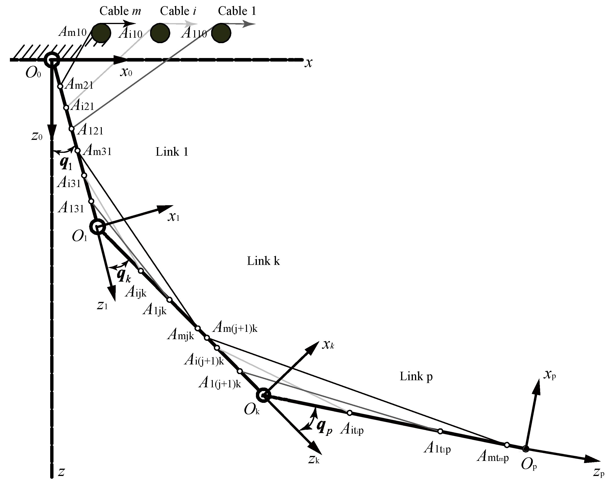
2. Dynamics Modelling
2.1. Dynamics Modelling of the Actuating Cables and Robot Body
- During the movement of the CDSM, the section where the cable bends is defined as the attachment point.
- The section of the cable between two adjacent attachment points is defined as the cable segment.
- The attachment point denotes the -th () attachment point of Cable () on Link (), where is the link number where the -th attachment point is located, is the total number of attachment points of Cable and is the total number of actuation cables.
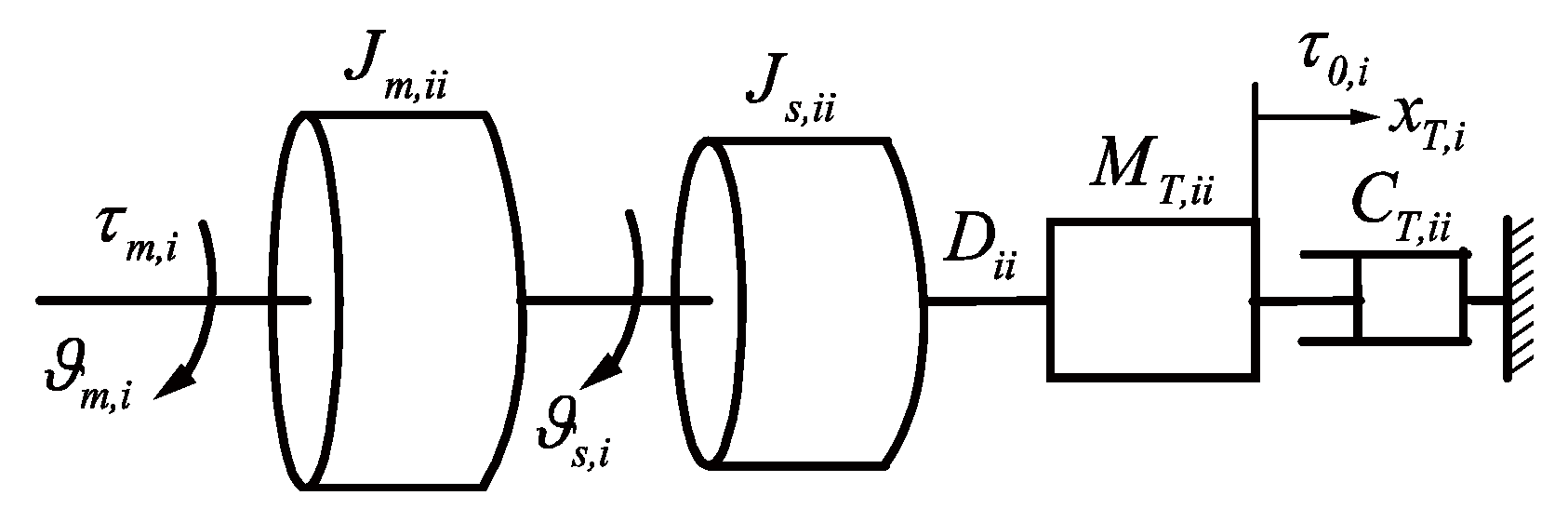
2.2. Dynamics Modelling of the Transmission Mechanism
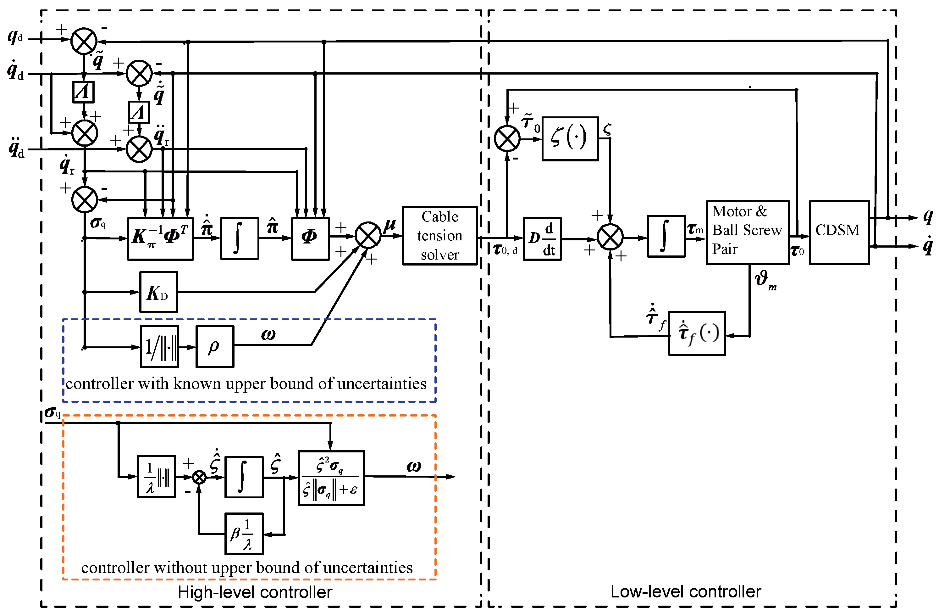
3. System Overview
4. Adaptive Robust Control
4.1. Adaptive Robust Control of Cable Tensions
4.2. Adaptive Robust Control of Motor Torque Outputs
5. Stability Analysis of Cascaded System
6. Experiment
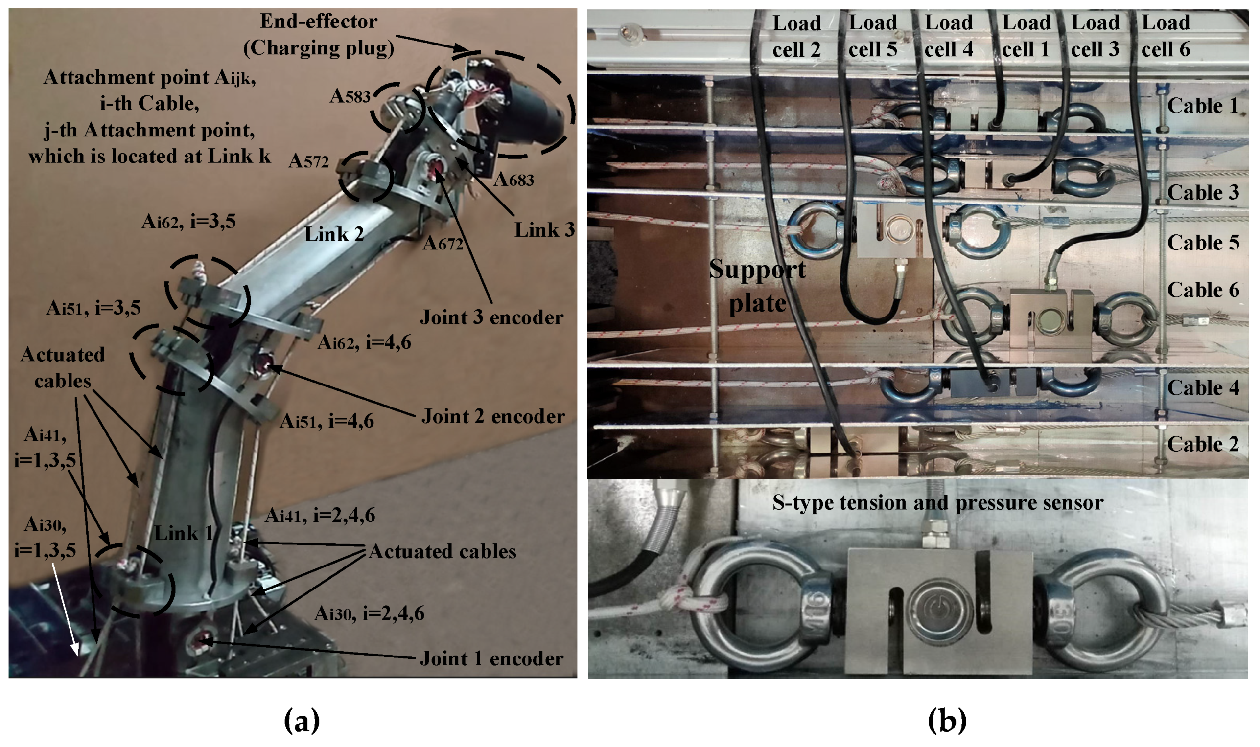
6.1. Experimental Setup
6.2. Experimental Results
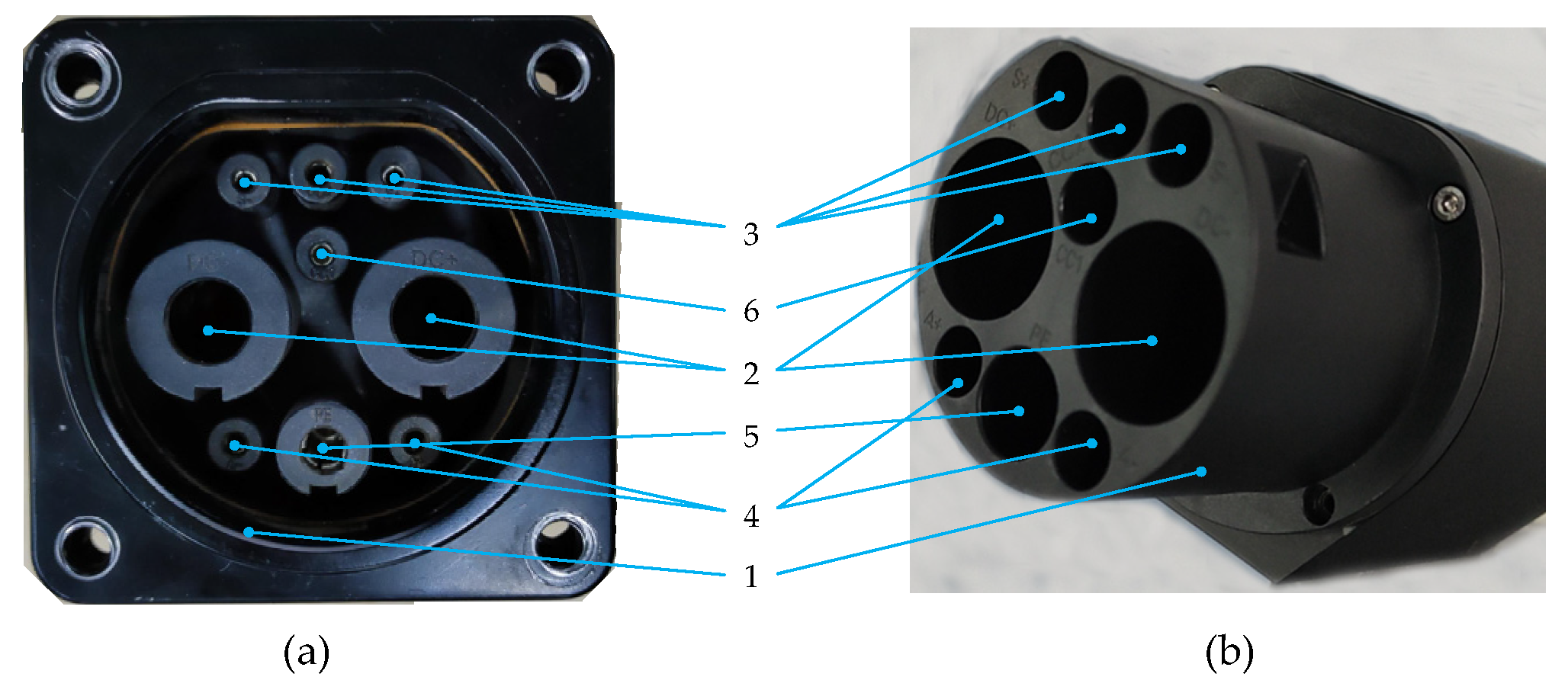
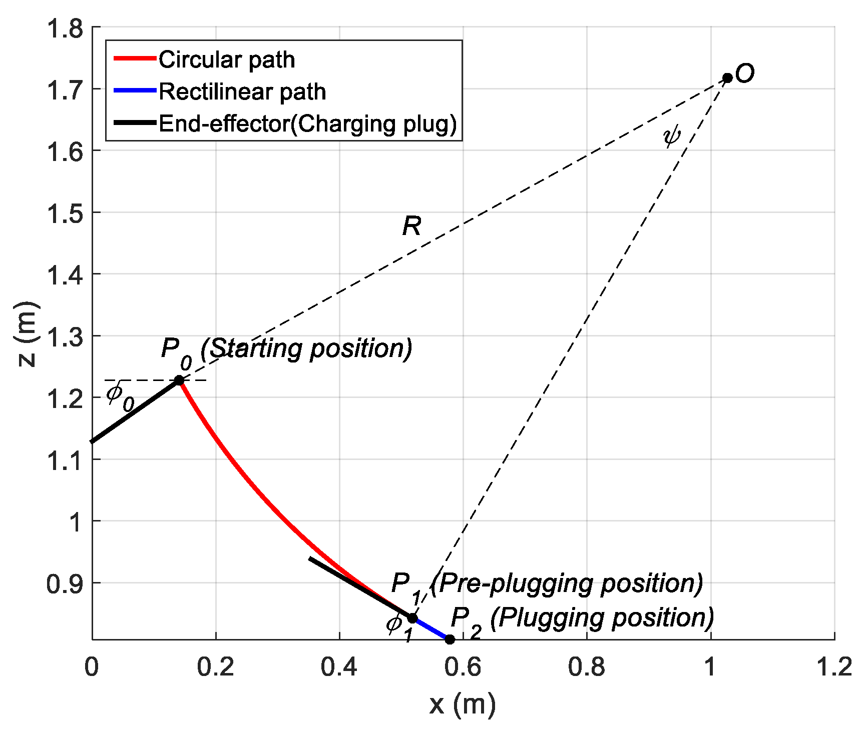
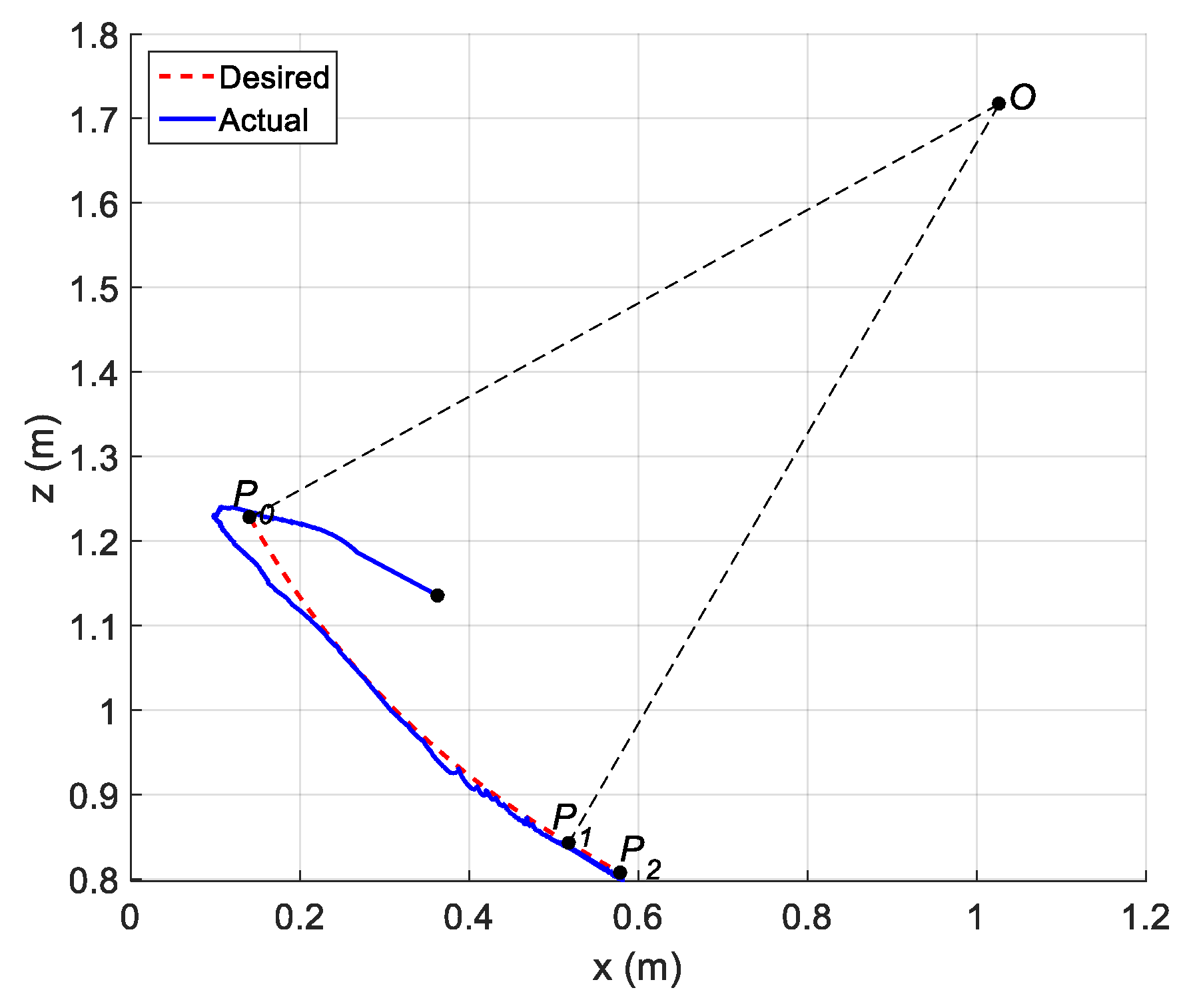
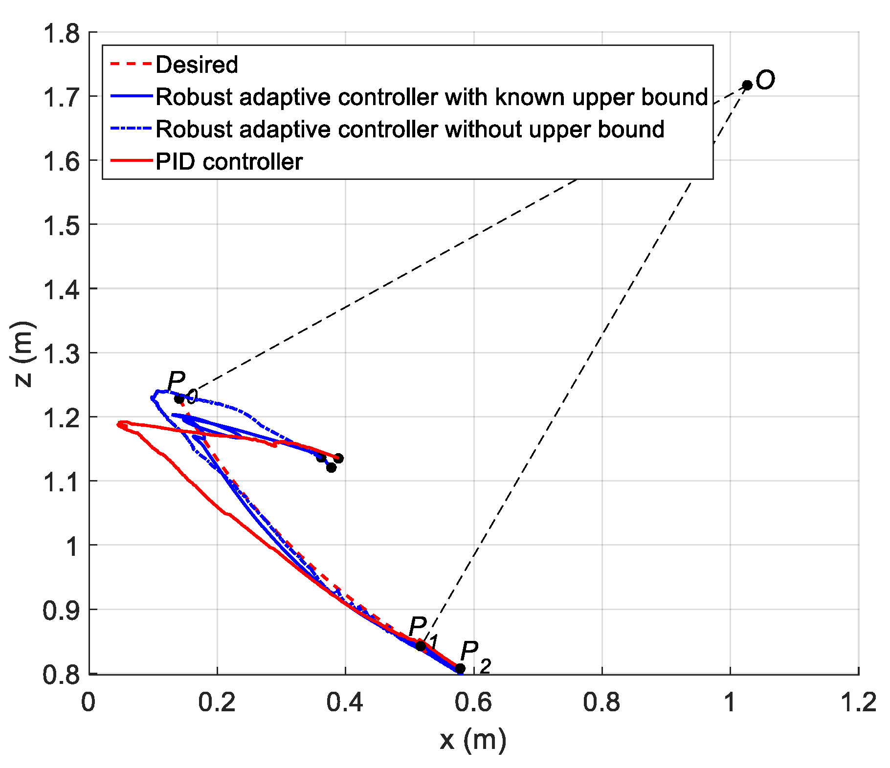
6.2.1. Path and Trajectory to Be Tracked
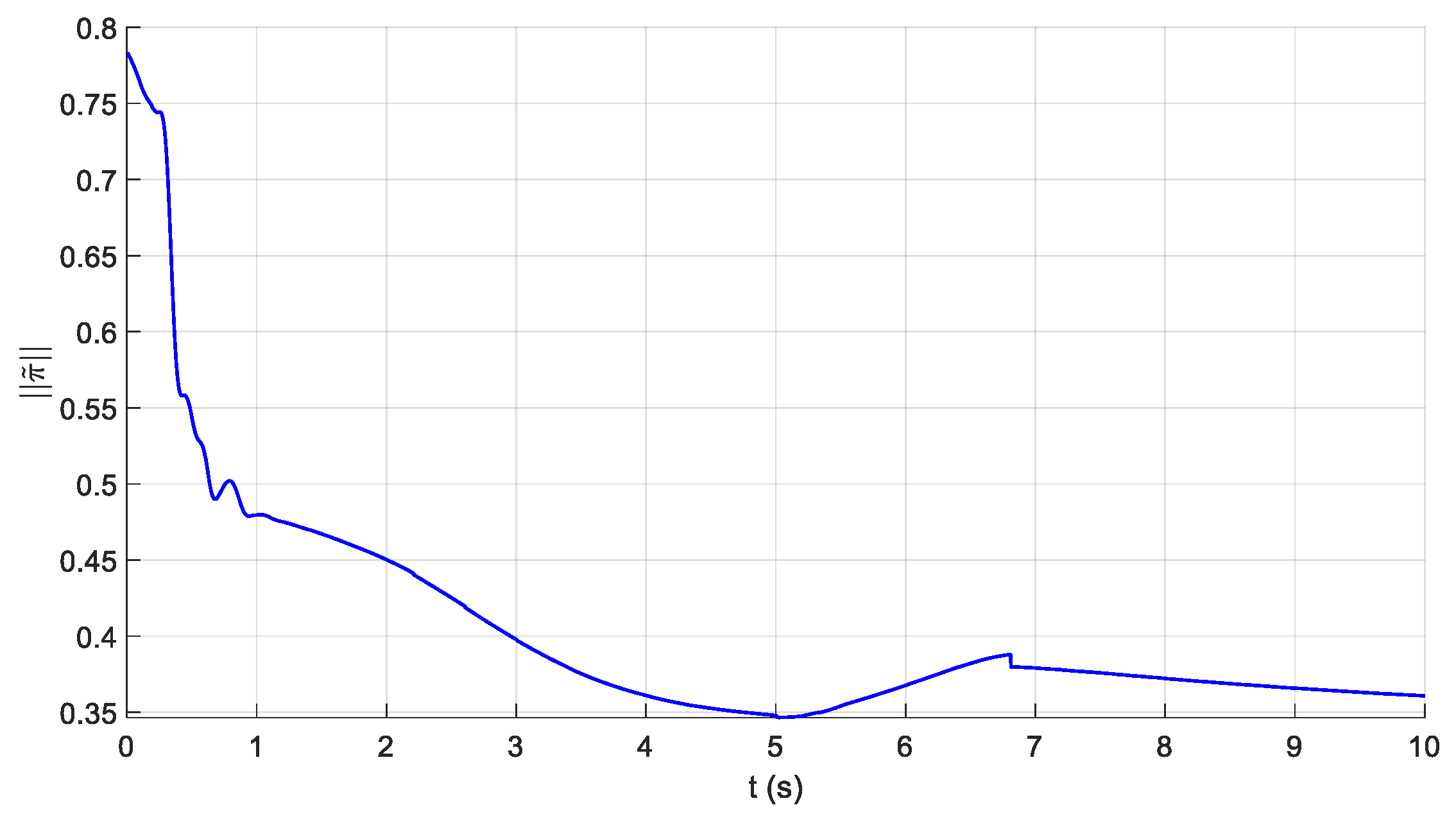
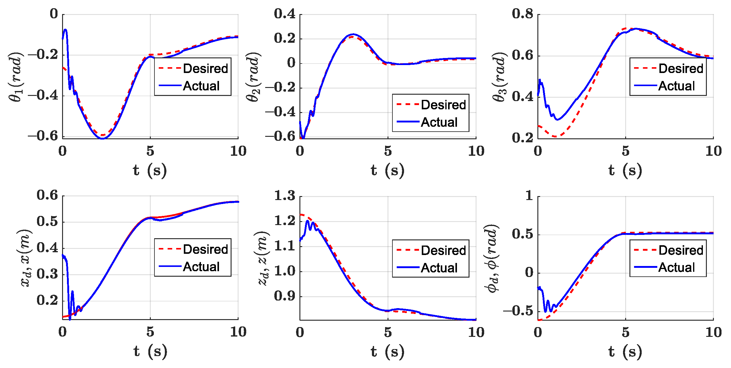
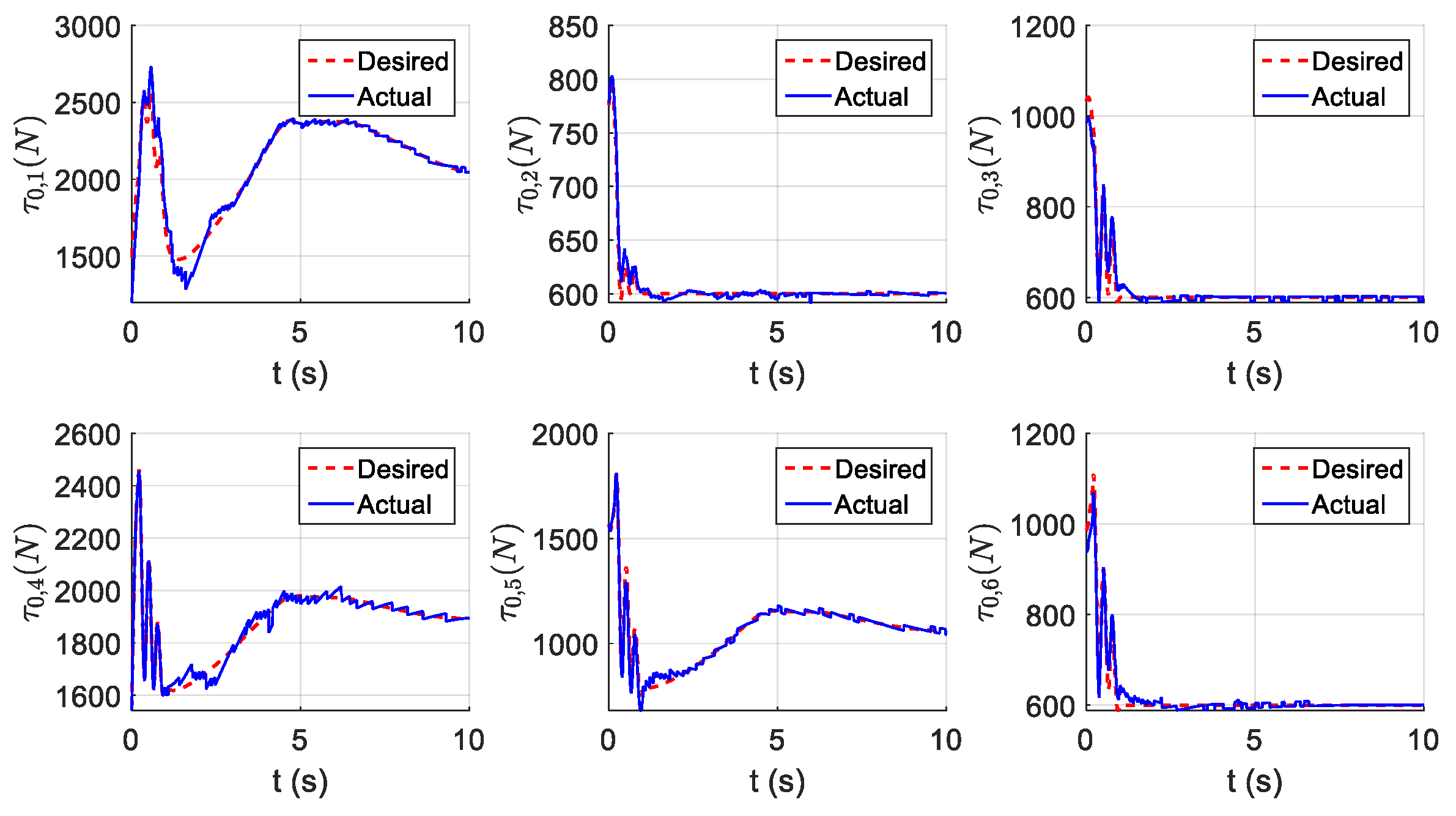
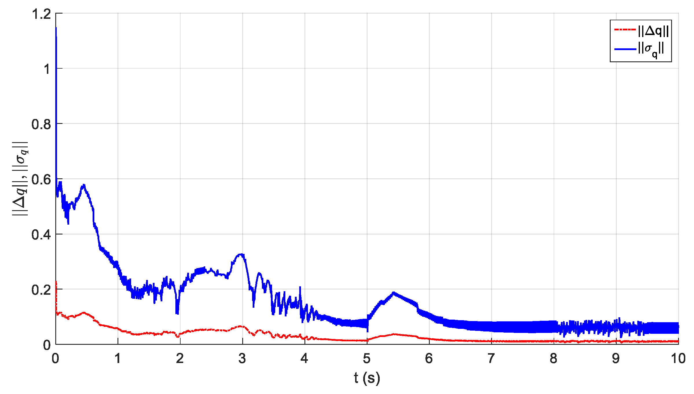
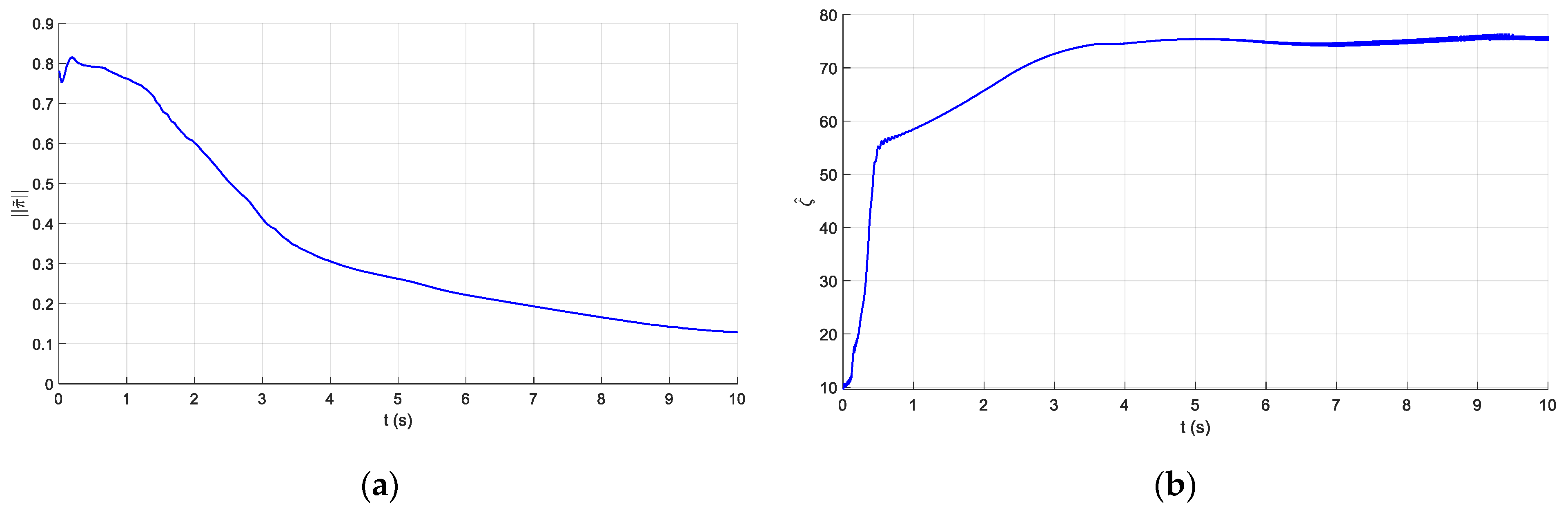
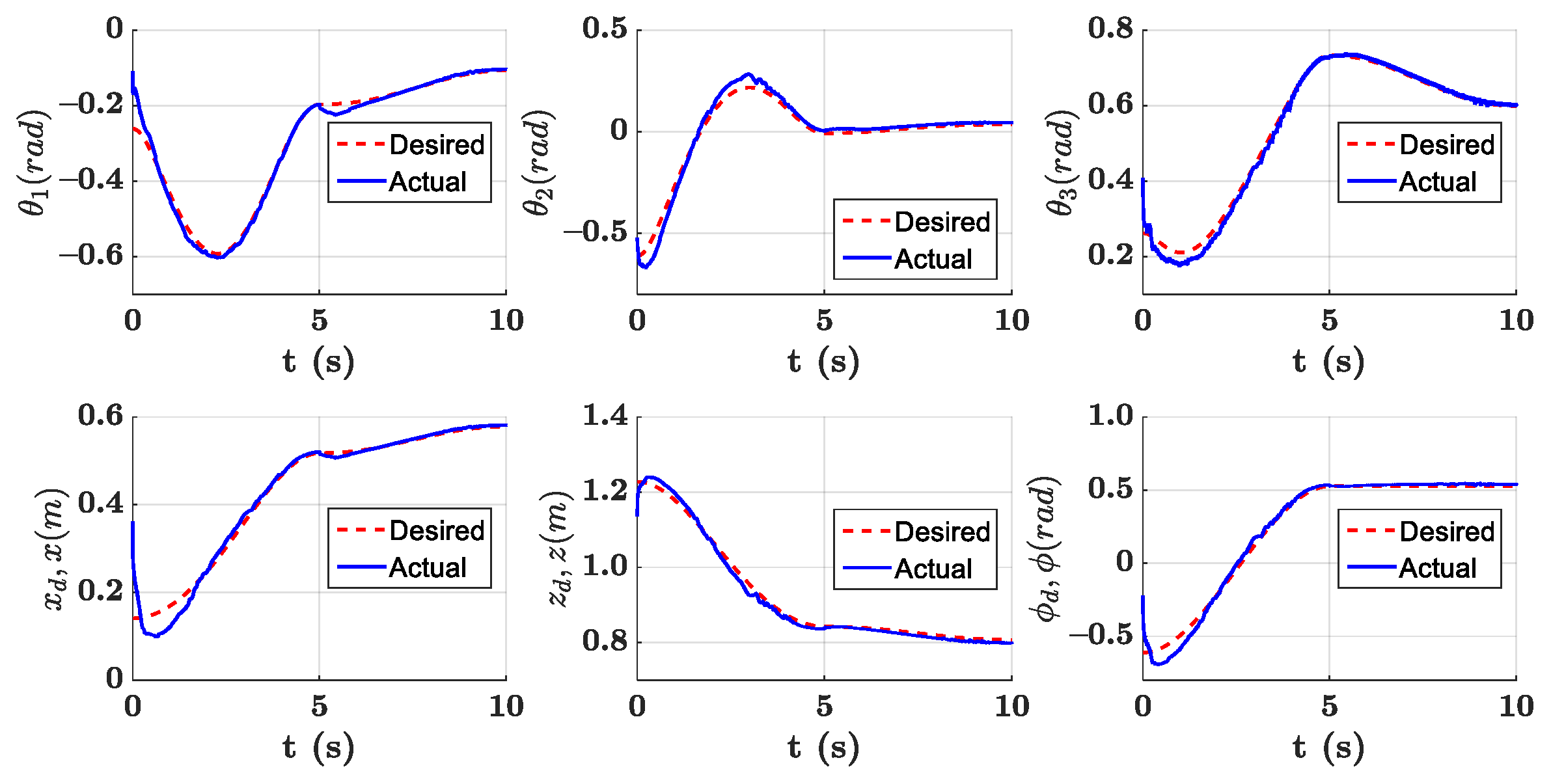
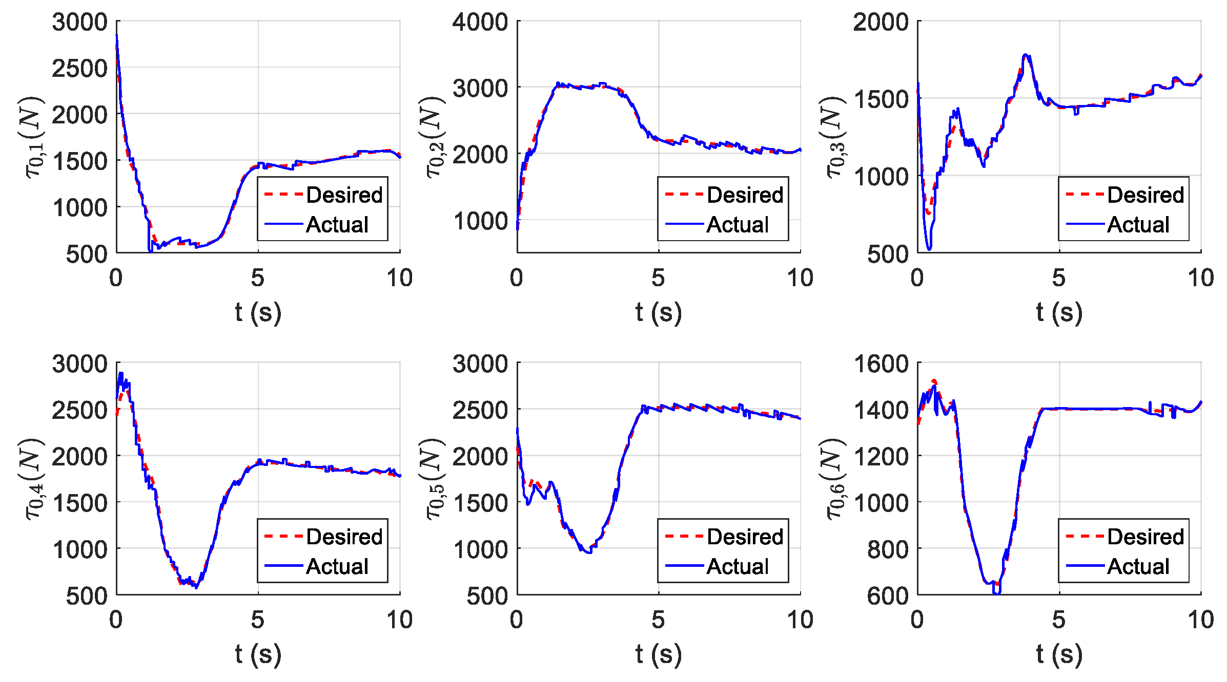
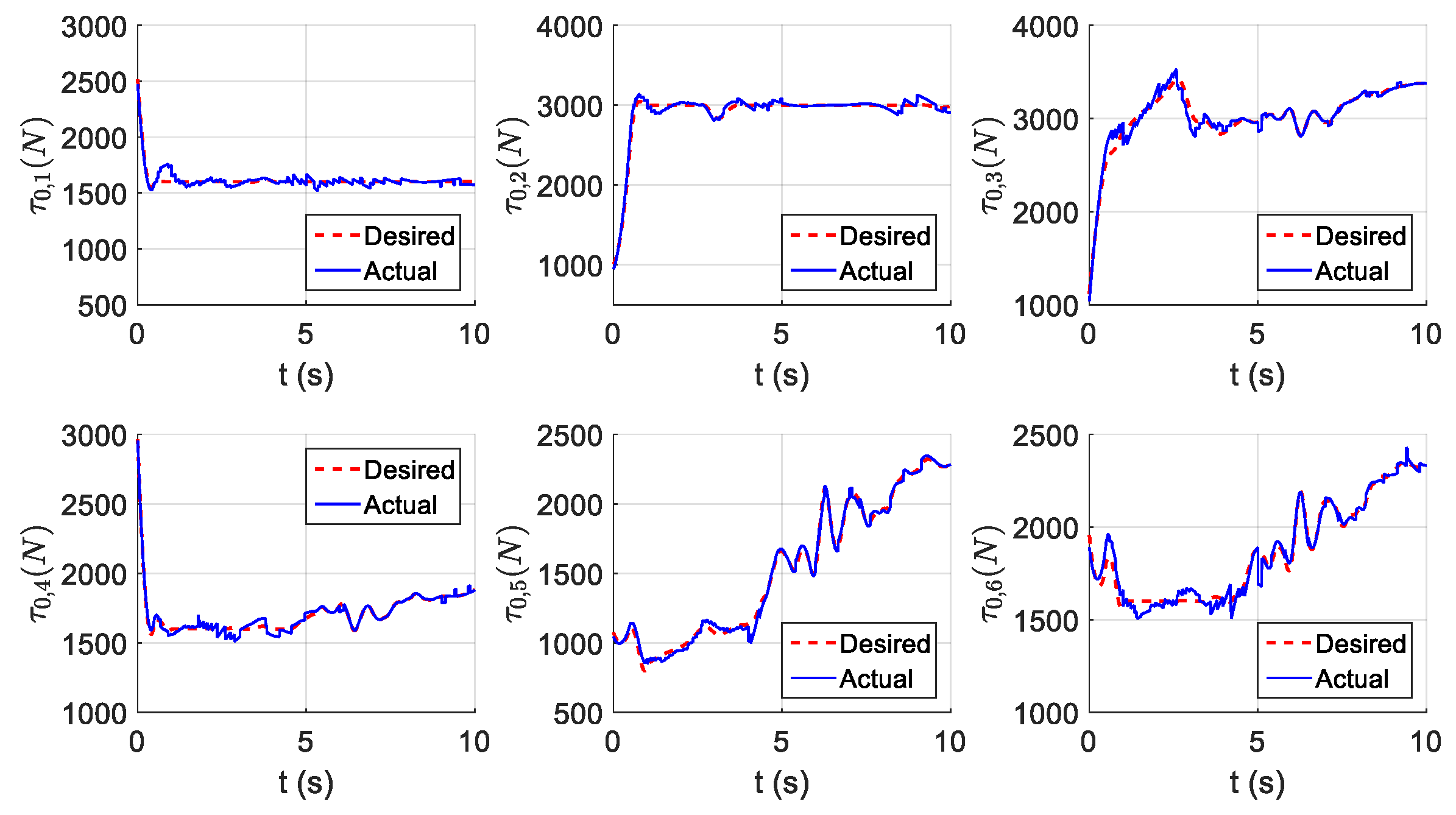
6.2.2. Results of the Controller with a Known Upper Bound of Uncertainties
6.2.3. Results of the Controller without an Upper Bound of Uncertainties
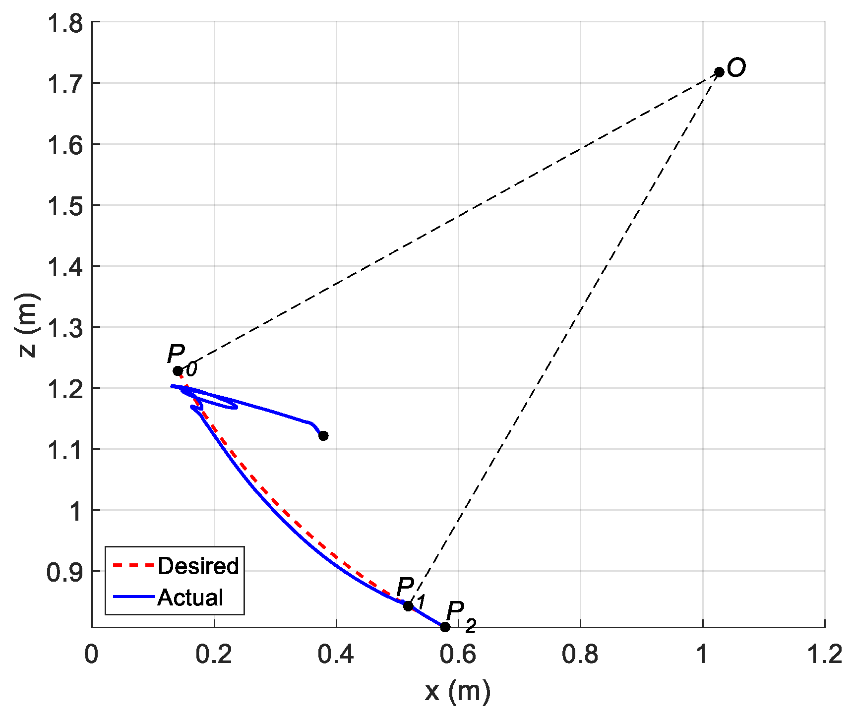
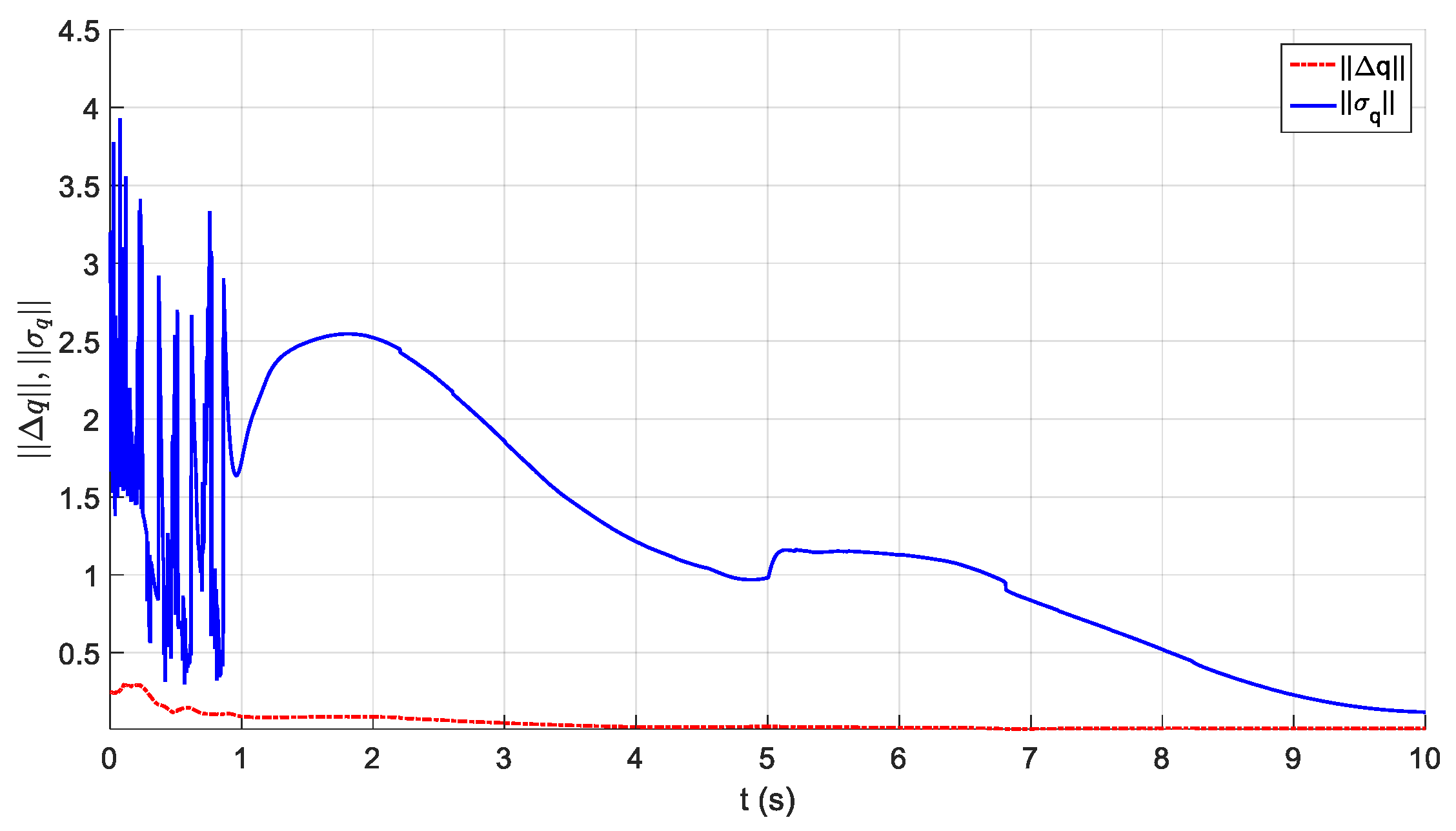
6.2.4. Results of the PID Controller
7. Conclusions
Author Contributions
Funding
Institutional Review Board Statement
Informed Consent Statement
Data Availability Statement
Acknowledgments
Conflicts of Interest
Appendix A
Appendix B
References
- Bryson, J.T. The Optimal Design of Cable-Driven Robots. Ph.D. Thesis, Department of Mechanical Engineering, University of Delaware, Newark, DE, USA, 2016. [Google Scholar]
- Cui, X.; Chen, W.; Jin, X.; Agrawal, S.K. Design of a 7-DOF cable-driven arm exoskeleton (carex-7) and a controller for dexterous motion training or assistance. IEEE ASME Trans. Mech. 2017, 22, 161–172. [Google Scholar] [CrossRef]
- Yao, Y.; Du, Z.; Wei, Z. Research on the snake-arm robot assembly system. Aeron. Manuf. Technol. 2015, 21, 26–30. [Google Scholar]
- Buckingham, R.; Chitrakaran, V.; Conkie, R. Snake-Arm Robots: A New Approach to Aircraft Assembly. SAE Technical Paper; SAE International: New York, NY, USA, 2007; pp. 1–3870. [Google Scholar]
- Lou, Y.; Di, S. Design of a cable-driven auto-charging robot for electric vehicles. IEEE Access 2020, 8, 15640–15655. [Google Scholar] [CrossRef]
- Buckingham, R.; Graham, A. Nuclear snake-arm robots. Ind. Robot. 2012, 39, 6–11. [Google Scholar] [CrossRef]
- Mustafa, S.K.; Agrawal, S.K. On the force-closure analysis of n-dof cable-driven open chains based on reciprocal screw theory. IEEE T. Robot. 2012, 28, 22–31. [Google Scholar] [CrossRef]
- Tsai, L.W. Design of tendon-driven manipulators. J. Vib. Acoust. 1995, 117, 80–86. [Google Scholar] [CrossRef]
- Cui, X.; Chen, W.; Yang, G.; Jin, Y. Closed-loop control for a cable-driven parallel manipulator with joint angle feedback. In Proceedings of the IEEE/ASME International Conference on Advanced Intelligent Mechatronics, Wollongong, Australia, 9–12 July 2013. [Google Scholar]
- Chen, W.; Cui, X.; Yang, G.; Chen, J.; Jin, Y. Self-feedback motion control for cable-driven parallel manipulators. Proc. Inst. Mech. Eng. Part C J. Mech. Eng. Sci. 2013, 228, 77–89. [Google Scholar] [CrossRef]
- Tang, L.; Wang, J.; Zheng, Y.; Gu, G.; Zhu, L.; Zhu, X. Design of a cable-driven hyper-redundant robot with experimental validation. Int. J. Adv. Robot. Syst. 2017, 14, 172988141773445. [Google Scholar] [CrossRef]
- Qi, R.; Khajepour, A.; Melek, W.W.; Lam, T.L.; Xu, Y. Design, kinematics, and control of a multijoint soft inflatable arm for human-safe interaction. IEEE Trans. Robot. 2017, 33, 594–609. [Google Scholar] [CrossRef]
- Xu, W.; Liu, T.; Li, Y. Kinematics, dynamics, and control of a cable-driven hyper-redundant manipulator. IEEE-ASME Trans. Mech. 2018, 23, 1693–1704. [Google Scholar] [CrossRef]
- Mao, Y.; Agrawal, S.K. Design of a cable-driven arm exoskeleton (carex) for neural rehabilitation. IEEE Trans. Robot. 2012, 28, 922–931. [Google Scholar] [CrossRef]
- Lau, D.; Oetomo, D.; Halgamuge, S.K. Inverse dynamics of multilink cable-driven manipulators with the consideration of joint interaction forces and moments. IEEE Trans. Robot. 2015, 31, 479–488. [Google Scholar] [CrossRef]
- Trevisani, A. Underconstrained planar cable-direct-driven robots: A trajectory planning method ensuring positive and bounded cable tensions. Mechatronics 2010, 20, 113–127. [Google Scholar] [CrossRef]
- Khosravi, M.A.; Taghirad, H.D. Robust PID control of fully-constrained cable driven parallel robots. Mechatronics 2014, 25, 87–97. [Google Scholar] [CrossRef]
- Babaghasabha, R.; Khosravi, M.A.; Taghirad, H.D. Adaptive robust control of fully-constrained cable driven parallel robots. Mechatronics 2015, 25, 27–36. [Google Scholar] [CrossRef]
- Jabbari, H.; Yoon, J. Robust trajectory tracking control of cable-driven parallel robots. Nonlinear Dyn. 2017, 89, 2769–2784. [Google Scholar] [CrossRef]
- Khalilpour, S.A.; Khorrambakht, R.; Taghirad, H.D. Robust cascade control of a deployable cable-driven robot. Mech. Syst. Signal. Pr. 2019, 127, 513–530. [Google Scholar] [CrossRef]
- Hong, H.; Ali, J.; Ren, L. A review on topological architecture and design methods of cable-driven mechanism. Adv. Mech. Eng. 2018, 10, 1–14. [Google Scholar] [CrossRef]
- Bruno, S.; Lorenzo, S.; Luigi, V.; Giuseppe, O. Robotics Modelling, Planning and Control, 1st ed.; Springer: London, UK, 2009; pp. 257–264. [Google Scholar]
- Khalil, H.K. Adaptive output feedback control of nonlinear systems represented by input-output models. IEEE Trans. Autom. Control 1996, 41, 177–188. [Google Scholar] [CrossRef]
- Corless, M.; Leitmann, G. Continuous state feedback guaranteeing uniform ultimate boundedness for uncertain dynamic systems. IEEE Trans. Autom. Control 1981, 26, 1139–1144. [Google Scholar] [CrossRef]
- Fischer, N.; Dani, A.; Sharma, N. Saturated control of an uncertain nonlinear system with input delay. Automatica 2013, 49, 1741–1747. [Google Scholar] [CrossRef]
- Xian, B.; Dawson, D.M.; Queiroz, M.S. A continuous asymptotic tracking control strategy for uncertain nonlinear systems. IEEE Trans. Autom. Control 2004, 49, 1206–1211. [Google Scholar] [CrossRef]
- Sepulchre, R.; Jankovic, M.; Kokotovic, P.V. Constructive Nonlinear Control, 1st ed.; Springer: New York, NY, USA, 2011. [Google Scholar]
- Chaillet, A.; Loría, A. Uniform semiglobal practical asymptotic stability for non-autonomous cascaded systems and applications. Automatica 2008, 44, 337–347. [Google Scholar] [CrossRef]
- Jankovic, M.; Sepulchre, R.; Kokotovic, P.V. Constructive Lyapunov stabilization of nonlinear cascade systems. IEEE Trans. Autom. Control 1996, 41, 1723–1735. [Google Scholar] [CrossRef]
- Zhao, B.; Xian, B.; Zhang, Y. Nonlinear robust adaptive tracking control of a quadrotor uav via immersion and invariance methodology. IEEE Trans. Ind. Electron. 2015, 62, 2891–2902. [Google Scholar] [CrossRef]
- Walzel, B.; Sturm, C.; Jürgen, F.; Hirz, M. Automated robot-based charging system for electric vehicles. In Proceedings of the 16 Internationales Stuttgarter Symposium, Stuttgarter, Germany, 28 April 2016; Bargende, M., Reuss, H.C., Wiedemann, J., Eds.; Springer: Wiesbaden, Germany, 2016. [Google Scholar]
- Miseikis, J.; Ruther, M.; Walzel, B.; Hirz, M.; Brunner, H. 3d vision guided robotic charging station for electric and plug-in hybrid vehicles. In Proceedings of the OAGM and ARW Joint Workshop 2017 on Vision, Automation and Robotics, Vienna, Austria, 15 March 2017. [Google Scholar]


| Math Symbol | Physical Meaning | Comment |
|---|---|---|
| Inertia matrix | Dynamic parameters of the CDSM | |
| Centrifugal and Coriolis matrices | ||
| Diagonal matrix of viscous friction coefficients | ||
| Vector of the gravity term | ||
| Jacobian matrix relating to | Jacobian matrices | |
| to joint moments | ||
| and | ||
| to joint moments | ||
| Regression matrix | Linearity in the dynamic parameters | |
| Vector of constant dynamic parameters | ||
| Vector of joint position, velocity, acceleration | tracked by high-level controller | |
| Vector of the input cable tensions | tracked by low-level controller | |
| Vector of motor torque outputs | Controller design object of low-level controller in Equation (58) | |
| Control input of joint moment | Controller design in Equation (15) | |
| Tracking errors of joint positions, input cable tensions | - | |
| Parameters of the high-level controller with a known upper bound of uncertainties. They meet the condition of Equation (23). | In Equation (16) | |
| In Equation (15) | ||
| In Equation (19) | ||
| In Equation (18) | ||
| In Equation (52) | ||
| Parameters of the high-level controller without an upper bound of uncertainties. They meet the condition of Equation (24). | In Equation (16) | |
| In Equation (15) | ||
| In Equation (21) | ||
| In Equation (22) | ||
| In Equation (20) | ||
| Low-level controller parameters which meet the condition of Equation (64) | In Equation (54) | |
| In Equation (59) |
| Parameter | Value | Unit |
|---|---|---|
| 5.0581, 4.7451, 3.4377 | kg | |
| 0.067485, 0.074783, 0.025347 | kg·m2 | |
| m | ||
| m | ||
| m | ||
| m/rad | ||
| kg·m2 | ||
| kg·m2 | ||
| kg |
| Parameter | Value | Unit |
|---|---|---|
| 5 | - | |
| - | ||
| - | ||
| 130 | - | |
| 0.04 | - | |
| Same as | ||
| - | ||
| - | ||
| - |
| Parameter | Value | Unit |
| 0.8 | - | |
| 5 | - | |
| - | ||
| 0.5 | - | |
| 0.01 | - | |
| 0.01 | - | |
| 0.04 | - | |
| Same as | ||
| 15 | Nm |
Publisher’s Note: MDPI stays neutral with regard to jurisdictional claims in published maps and institutional affiliations. |
© 2021 by the authors. Licensee MDPI, Basel, Switzerland. This article is an open access article distributed under the terms and conditions of the Creative Commons Attribution (CC BY) license (http://creativecommons.org/licenses/by/4.0/).
Share and Cite
Lou, Y.; Lin, H.; Quan, P.; Wei, D.; Di, S. Robust Adaptive Control of Fully Constrained Cable-Driven Serial Manipulator with Multi-Segment Cables Using Cable Tension Sensor Measurements. Sensors 2021, 21, 1623. https://doi.org/10.3390/s21051623
Lou Y, Lin H, Quan P, Wei D, Di S. Robust Adaptive Control of Fully Constrained Cable-Driven Serial Manipulator with Multi-Segment Cables Using Cable Tension Sensor Measurements. Sensors. 2021; 21(5):1623. https://doi.org/10.3390/s21051623
Chicago/Turabian StyleLou, Ya’nan, Haoyu Lin, Pengkun Quan, Dongbo Wei, and Shichun Di. 2021. "Robust Adaptive Control of Fully Constrained Cable-Driven Serial Manipulator with Multi-Segment Cables Using Cable Tension Sensor Measurements" Sensors 21, no. 5: 1623. https://doi.org/10.3390/s21051623
APA StyleLou, Y., Lin, H., Quan, P., Wei, D., & Di, S. (2021). Robust Adaptive Control of Fully Constrained Cable-Driven Serial Manipulator with Multi-Segment Cables Using Cable Tension Sensor Measurements. Sensors, 21(5), 1623. https://doi.org/10.3390/s21051623