Abstract
Removing bounding surfaces such as walls, windows, curtains, and floors (i.e., super-surfaces) from a point cloud is a common task in a wide variety of computer vision applications (e.g., object recognition and human tracking). Popular plane segmentation methods such as Random Sample Consensus (RANSAC), are widely used to segment and remove surfaces from a point cloud. However, these estimators easily result in the incorrect association of foreground points with background bounding surfaces because of the stochasticity of randomly sampling, and the limited scene-specific knowledge used by these approaches. Additionally, identical approaches are generally used to detect bounding surfaces and surfaces that belong to foreground objects. Detecting and removing bounding surfaces in challenging (i.e., cluttered and dynamic) real-world scenes can easily result in the erroneous removal of points belonging to desired foreground objects such as human bodies. To address these challenges, we introduce a novel super-surface removal technique for complex 3D indoor environments. Our method was developed to work with unorganized data captured from commercial depth sensors and supports varied sensor perspectives. We begin with preprocessing steps and dividing the input point cloud into four overlapped local regions. Then, we apply an iterative surface removal approach to all four regions to segment and remove the bounding surfaces. We evaluated the performance of our proposed method in terms of four conventional metrics: specificity, precision, recall, and F1 score, on three generated datasets representing different indoor environments. Our experimental results demonstrate that our proposed method is a robust super-surface removal and size reduction approach for complex 3D indoor environments with scores of the four evaluation metrics ranging between 90% and 99%.
1. Introduction
In image processing, background subtraction is widely used in object detection and tracking approaches [1,2,3] with broad applications such as human tracking [4,5], face recognition [6], traffic management [7], and surveillance systems [8,9]. Background subtraction is typically a preprocessing phase used to identify and differentiate the foreground pixels (representing objects of interest) from the background pixels (representing uninteresting information). The background pixels can then be subtracted or removed from the original image, leaving only the foreground pixels, which reduces the storage space requirements, reduces the computational complexity, and improves the overall algorithm performance of downstream image processing techniques. Established 2D background subtraction approaches are based on static background segmentation methods [10], adaptive Gaussian mixture models [11,12], real-time codebook models [13,14], and independent component analysis-based techniques [15,16]. Although advanced 2D background subtraction techniques can handle gradual illumination changes and repetitive movements in the background, they perform poorly in the presence of shadows or foreground regions with colors similar to the background [17]. The release of commercially available and inexpensive depth sensors such as the Microsoft Kinect opened new doors for improved background subtraction techniques because of the availability of additional depth data associated with each pixel of color data. Depth sensor (RGB-D) systems are more robust for background detection problems compared to classic color-based systems because depth data are largely invariant to color, texture, shape, and lighting [18,19]. As a result of the advantages of combined depth and color information, data from RGB-D sensors have also been widely used in background segmentation methods (e.g., [17,20,21]) which have been thoroughly reviewed (see [22] for a comprehensive review of different 3D background subtraction methods and their capabilities in solving common background segmentation challenges).
Background subtraction methods are generally used to analyze individual images and identify the foreground by first estimating a reference background that is developed from historical information obtained from videos or sequences of images. Therefore, the classic application of 2D background subtraction is separating dynamic or moving objects from a relatively static or slow-changing background scene. However, RGB images only contain intensity information and spatial information that is largely restricted to the two dimensions of the image that are perpendicular to the camera’s perspective. Accordingly, identifying the boundaries between objects, or conversely identifying object interactions or contact, is limited mainly to detectable intensity differences. In applications that utilize RGB-D data, interactions or contact between objects and object spatial relationships can be more directly measured.
Furthermore, registration between depth and RGB data allows traditional 2D background subtraction approaches to be supplemented with additional depth-based approaches (e.g., [23,24]), and further allows RGB-D data to be represented as 3D point clouds [25]. For example, reliably identifying and removing static background components such as roads and walls before modeling the background can result in both improved background subtraction and improved foreground segmentation using both 2D and RGB-D data; these improvements, to our knowledge, have only been realized through approaches that require additional data and computation, such as motion estimation between consecutive frames (e.g., [26]). Identifying static background components suffers from the same limitations as modeling the entire background using 2D data, suggesting that little benefit is afforded by first removing these background objects, then modeling the background. However, with RGB-D data, parametrically modeled objects (e.g., planes, spheres, cones, cylinders, and cubes) are far more reliably detectable. As a result, researchers have attempted to segment or remove large planar surfaces (e.g., walls, ceiling, and floor surfaces) as a preprocessing or fundamental step before all other algorithms (e.g., [27,28,29]).
In general, large planar surfaces comprise a large percentage of points within each frame of RGB-D data captured in indoor environments. However, outside specific applications that seek to identify significant surfaces (e.g., ground plane detection [30]), large planar surfaces are not often the objects of interest in 3D computer vision applications. Notably, smaller planar surfaces (e.g., tabletops, chair seats and backs, desks) are more likely to be of interest than larger surfaces at the boundaries of the scene. Furthermore, the large bounding surfaces can decrease the performance of 3D computer vision algorithms (e.g., object segmentation and tracking) by cluttering their search space. Therefore, a robust removal technique for points that belong to surfaces at the outer boundaries of the RGB-D data can significantly reduce the search space and bring three main benefits to the computer vision systems: improving downstream results, speeding up downstream processes, and reducing the overall size of the point clouds. We refer to these large surfaces, which may include points from multiple planes or objects (e.g., points that represent a wall, window, or curtain) at the extremes of the point clouds as super-surfaces in the context of background subtraction applications. Our objective is to develop a robust technique of removing super-surfaces from RGB-D data captured from indoor environments and represented as point clouds. Our intention is that our super-surface removal technique will function as a pre-processing step, improving existing computer vision techniques, and reducing storage requirements, without removing any foreground data.
1.1. Related Work
Point cloud data are classified as either organized or unorganized datasets. Organized datasets are represented by a matrix-like structure, where the data (i.e., voxels) are accessible by index, usually according to their spatial or geometric relationship. Unlike organized point clouds, the relationships between adjacent voxels of unorganized datasets are unknown, and the data are simply stored as a one-dimensional, unsorted array. Data from RGB-D sensors are typically stored as organized point clouds, where indices are referenced according to the spatial resolution of the sensor. However, point cloud pre-processing steps such as down-sampling often produce unorganized point clouds. While it is trivial to convert an organized point cloud to an unorganized point cloud, the reverse is much more complicated and costly. Since spatial relationships between voxels are preserved, plane detection is less challenging for organized point clouds. However, computer vision approaches designed for unorganized datasets are universal [31] (i.e., they can also be used for organized datasets), so a robust plane detection approach must work with unorganized datasets and not rely on the spatial relationship of voxels derived from their storage indices. In general, plane segmentation methods can be categorized into three categories: model fitting-based methods, region growing-based methods, and clustering feature-based methods.
1.1.1. Model Fitting-Based Methods
Random Sample Consensus (RANSAC) [32] and Hough transform [33] are the most commonly used model fitting-based methods for plane segmentation. The Hough transform is a voting technique for identifying objects that can be modeled parametrically, such as lines, planes, and spheres. Every point is transformed into a unique function (e.g., a sinusoid when modeling lines) in a discretized parameter space. Objects of interest can then be extracted by selecting the maximal intersections between the functions in the discretized parameter space, where the spatial tolerance for model fitting (e.g., to compensate for sensor resolution, noise, and object surface variations) can be accommodated by changing the resolution of the parameter space. The Hough transform has been successfully used for 3D plane segmentation in several publications (e.g., [34,35]). Unfortunately, although Hough transform-based methods can robustly segment 3D objects, they necessitate large amounts of memory and significant computational time [36], and their results depend significantly on the proper selection of segmentation parameters [37]. More importantly, Hough transform is unable to discriminate between voxels that lie within a parameterized model (i.e., inliers) and outside the model (i.e., outliers) since spatial relationships are not preserved in the Hough parameter space. The result is that foreground points that belong to objects that are spatially close to the parameterized background model will often be associated with the model, and ultimately the background scene.
The RANSAC algorithm begins with a random selection of data points that estimate the corresponding model parameters (e.g., three points for a plane). Then, the remaining points are examined to determine how many of them are well-approximated by the model. Finally, the RANSAC algorithm returns the model with the highest percentage of inliers that are within a fixed threshold (e.g., the orthogonal distance from the planar model). Many researchers have proposed RANSAC-based algorithms for 3D plane segmentation, such as [37,38,39].
Awwad et al. [37] proposed a RANSAC-based segmentation algorithm that first clusters the data points into small sections based on their normal vectors and then segments the planar surfaces. This implementation of RANSAC prevents the segmentation of spurious surfaces in the presence of parallel-gradual planes such as stairs. Chen et al. [38] developed an improved RANSAC algorithm through a novel localized sampling technique and a region growing-based approach. Their proposed method, intended to segment polyhedral rooftops from noisy Airborne Laser Scanning (ALS) point clouds, is based on the assumption that rooftops comprise only planar primitives. Li et al. [39] proposed an enhanced RANSAC algorithm based on Normal Distribution Transformation (NDT) cells to prevent segmenting spurious planes. The algorithm considers each NDT cell rather than each point. After dividing the data points into a grid of NDT cells, a combination of the RANSAC algorithm and an iterative reweighted least-square approach fit a plane in each cell. Finally, a connected-component approach extracts large planes and eliminates points that do not belong to planes. Although the proposed method can detect 3D planes more reliable and faster than the standard RANSAC, it requires cell size tuning for different datasets.
According to a performance comparison by Tarsha-Kurdi et al. [40], the RANSAC algorithm outperforms the Hough transform approach for 3D roof plane segmentation in terms of both speed and accuracy. However, RANSAC suffers from spurious plane detection in complex 3D indoor environments [39].
1.1.2. Region Growing-Based Methods
In general, region growing-based methods have two main stages. First, they pick a seed point and then merge the neighboring points or voxels that comply with the predefined criteria (e.g., similar normal vector). Several researchers proposed point-based, voxel-based, and hybrid region growing techniques for 3D point cloud segmentation. Tóvári and Pfeifer [41] proposed a point-based region growing algorithm that merges adjacent points to a seed region based on their normal vectors and distance to the adjusting plane. Nurunnabi et al. [42] utilized the same criteria but with a different seed point selection approach and a better normal vector estimation.
Voxel-based region growing algorithms (e.g., [43,44]) improve the speed and robustness of point-based methods by voxel-wise processing of the 3D point clouds. Xiao et al. [45] proposed a 3D plane segmentation method based on a hybrid region growing approach utilizing a subwindow and a single point as growth units. Although their technique is significantly faster than the point-based region growing approach, it was only intended for organized point clouds. Vo et al. [36] proposed a fast plane segmentation technique for urban environments. The method consists of two main stages: first, a coarse segmentation is achieved using an octree-based region growing approach, then a point-based process refines the results by adding unassigned points into incomplete segments.
Region growing-based methods are easy to employ for 3D plane segmentation, primarily for organized point clouds. However, their output results depend on the growing criteria, the seed point selection, and the textures or roughness of planes [46]. Furthermore, they are not robust to occlusion, point density variation, and noise [47].
1.1.3. Clustering Feature-Based Methods
Clustering feature-based methods adopt a data clustering approach based on characteristics of planar surfaces, such as normal vector attributes. Filin [48] proposed a clustering method based on an attribute vector comprising a point location, its tangent plane’s parameters, and the height difference between the point and its adjacent points. In another work, Filin and Pfeifer [49] computed point features using a slope adaptive neighborhood system and employed a mode-seeking algorithm to extract clusters. Then, they extended or merged these clusters with their adjacent points or clusters if they shared analogous standard deviations and surface parameters. Czerniawski et al. [28] applied a simple density-based clustering algorithm to a normal vector space (i.e., a Gaussian sphere). The dense clusters on the Gaussian sphere represent the directions perpendicular to large planes. Zhou et al. [50] proposed a clustering feature-based method for segmenting planes in terrestrial point clouds. First, they created a 4D parameter space using the planes’ normal vectors and their distance to the origin. Then, they segmented the planar surfaces by applying the Iso cluster unsupervised classification method.
Despite the efficiency of clustering feature-based methods, employing multi-dimensional features in large point clouds is computationally intensive [36]. Furthermore, they are sensitive to noise and outliers [51]. Moreover, the clustering segmentation approaches cannot reliably segment the edge points as these points may have different feature vectors compare to the surface points.
1.2. Contributions
Several 3D plane segmentation methods can satisfactorily detect different planar surfaces for various computer vision applications. However, to our knowledge, no approaches have been developed specifically for bounding surface removal, particularly in complex environments: environments that are cluttered, and where the placement of a depth sensor is not ideal. Additionally, existing segmentation approaches generally segment foreground points that belong to parametrically modeled objects of interest (e.g., planes, spheres, cones, cylinders, and cubes), rather than with the intention of removing background points belonging to the bounding surfaces. Therefore, existing approaches can easily remove critical foreground objects (or portions of foreground objects), significantly impacting the segmentation accuracy of semantic information. To overcome these limitations, we propose a method of removing background bounding surfaces (i.e., super-surfaces, such as walls, windows, curtains, and floor). Our novel method is particularly suited to more challenging and cluttered indoor environments, where differentiating between foreground and background points is complicated. Accordingly, our objective is to develop a robust background super-surface removal method that can support a wide range of sensor heights relative to the ground (i.e., support varied sensor perspectives) for organized and unorganized point clouds. Additionally, our approach must ensure that foreground objects, and points belonging to those objects, are preserved during super-surface removal.
Our method significantly reduces the search space, and it can considerably reduce the size of 3D datasets, depending on the number and size of the super-surfaces in each point cloud. Furthermore, when used as a preprocessing step, our approach can improve the results and the running time of different 3D computer vision methods such as object recognition and tracking algorithms. The remainder of this paper is organized as follows. In the next section, we describe our proposed 3D super-surface removal method. In Section 3, we provide our experimental results and the evaluation of our proposed method. In Section 4, we present our discussion and future work, followed by conclusions in Section 5.
2. The Iterative Region-Based RANSAC
Our iterative region-based RANSAC (IR-RANSAC) method has five main steps, as illustrated in Figure 1. We begin with two preprocessing techniques, first down-sampling the raw point cloud and then removing noisy or outlying points in the depth map. Second, we divide the point cloud space into four overlapped local regions based on the current view of the sensor. Third, we segment a base plane in each of the four local regions. Fourth, we implement an iterative plane removal technique to all four local regions, segmenting and removing the super-surfaces. Finally, we cluster the remaining point cloud using the geometric relationship between groups of points, resulting in a final point cloud comprised only of clustered objects of interest.
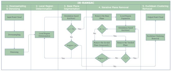
Figure 1.
The flowchart of IR-RANSAC.
2.1. Downsampling and Denoising
Since input point clouds are generally large in size due to the significant number of 3D points and associated color information, a downsampling method with low computational complexity can significantly reduce the running time of point cloud processing algorithms. Downsampling is typically achieved using either a random downsampling method [52] or a voxelized grid approach [53]. Although the former is more efficient, the latter preserves the shape of the point cloud better and exploits the geometric relationship of the underlying samples. Since we are predominantly concerned with preserving the underlying points that represent the true geometry of objects in the scene, we utilized a voxelized grid approach [53] that returns the centroid of all the points in each 3D voxel grid with a leaf size of 0.1 cm. In this way, the downsampled point clouds will still reflect the structure and maintain the geometric properties of the original point cloud while reducing the total amount of points that will need to be processed and stored.
Removing noisy points is a critical point cloud preprocessing task. Noisy or spurious points have two significant impacts on our approach. A noisy point cloud with false or spurious data points, including points outside of a scene’s real boundaries (see Figure 2 for example) can lead to a wrong measurement of the overall bounding box containing the point cloud, resulting in the definition of incorrect local regions in our subsequent processing steps. Furthermore, noisy points within the point cloud itself will effectively skew or change the geometry of the true objects. We utilized a statistical outlier removal approach [54] by examining the k-nearest neighbors () of each point, and removing all points with a distance () of more than one standard deviation of the mean distance to the query point to remove outliers of each captured point cloud. If the average distance of a point to its k-nearest neighbors is above the threshold (), it is considered as an outlier. In this way, we remove points that are dissimilar from other points in their neighborhood. Together, these approaches decrease the number of points in the point cloud, reducing the downstream processing time and increasing the accuracy of our process.
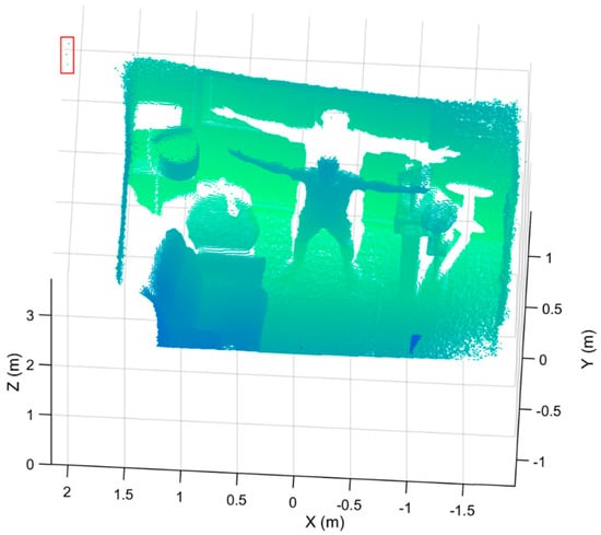
Figure 2.
A sample point cloud with false data points (surrounded by a red rectangle), detected as the noise outside the true boundaries of the room. These noise artifacts artificially expand the overall outer dimensions of the point cloud.
2.2. Local Region Determination
Dividing our captured point clouds into four local regions of interests, based on the properties of our indoor environments, reduces the possibility of detecting foreground planes, increases computational efficiency, and leverages the likely spatial location of potential bounding surfaces. In this way, we exploit knowledge of the scene based on the known sensor perspective, while allowing for surface locations to vary relative to each other in different rooms. Further, these regions help ensure that foreground objects that may appear planar in composition (e.g., tables, beds) are preserved and differentiated from background bounding surfaces.
We partition the point cloud space into four overlapped local regions based on the current view of the sensor. First, we find the bounding values of the downsampled and denoised point cloud, where the values and are the Euclidean extrema of the bounding box enclosing the point cloud, and are the Euclidean dimensions of the bounding box. Using the ranges defined in Table 1, we then determine the four local regions (see Figure 3 for a sample visualization of the local regions). We will use these four regions to identify, segment, and remove potential super-surfaces in each region.

Table 1.
Ranges for each local region.
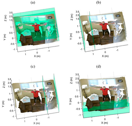
Figure 3.
The boundaries of the four local regions highlighted in green: (a) the back, (b) left, (c) right, and (d) bottom regions.
Since our approach must be independent of any prior knowledge about the geometry of the indoor environment and both the location and perspective of the sensor, the four initial local regions may not include all the points that are actually part of the super-surfaces (e.g., Figure 3d, where parts of the floor are not included within the local region).
Selecting larger initial regions will increase the likelihood that all true points are within the regions but will also increase the likelihood of including points belonging to foreground objects near the super-surfaces (e.g., beds and sofas). To resolve this issue, we implement conservative local regions and extend these four regions after base plane segmentation (see Section 2.4).
2.3. Base Plane Segmentation
We utilize the RANSAC algorithm [32] to segment the largest planes with a specific orientation in each of the local regions. All segmented plane candidates with more points than a learned value of the total number of points in the point cloud, are verified as base planes and stored for use in the next step (Section 2.4). Planes containing fewer than points may be associated with key objects or small bounding planes and are dealt with in subsequent processing steps. Furthermore, is set as a proportion of the total points such that it is adaptive to the size of the point cloud.
The RANSAC algorithm iteratively and randomly samples three voxels, as a minimum subset to generate a hypothesis plane. These three points represent two vectors and , and their cross product is the normal vector to the plane . Therefore, the three parameters of the plane () are computed, and can be solved. In each iteration, the algorithm computes the distance between all the remaining data points and the plane and then counts the number of points within a distance threshold ( of the plane. Finally, RANSAC returns the plane with the highest percentage of inliers.
We add an orientation constraint to the standard RANSAC algorithm (orientation-based RANSAC) so that we assign priority to segmented planes with the highest percentage of inliers that have an expected orientation relative to the local regions. To do this, we defined an initial reference vector for each of the local regions, aligned with the sensor axes as ,, and for the back, left, right, and bottom regions, respectively (Figure 4). Further, we define a maximum allowance angular variation ( degrees) between the normal vector of the planes and our reference vectors to allow for sensor perspective variations.
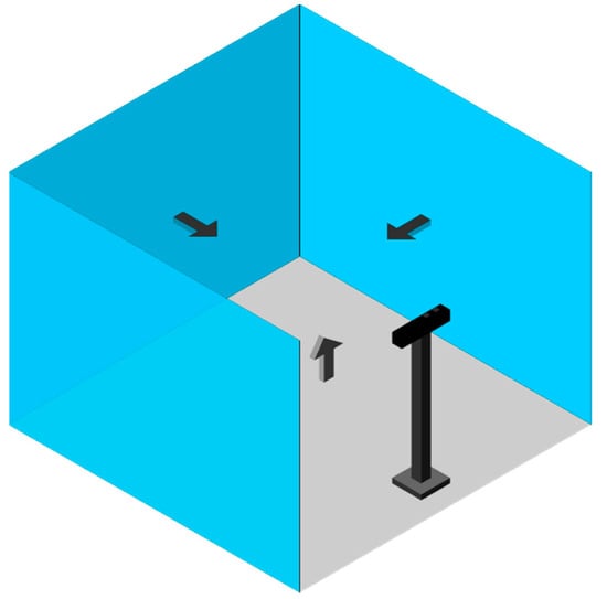
Figure 4.
The initial reference vectors.
The maximum number of iterations required for convergence by the RANSAC algorithm can be approximated as Equation (1) [55]. Convergence depends on the number of samples ( for the plane fitting), the target success probability (e.g., ), and the outlier ratio . Considering there is no prior knowledge about the underlying outlier ratio, it is difficult to approximate the number of RANSAC iterations. Based on our experimental results and due to the iterative design of IR-RANSAC, the algorithm works appropriately with the number of trials adhering to of the data points within each local region. In this study, we set to 2% of the data points (e.g., if the back region contains 60,000 points, the maximum number of trials will be set to 1200). Increasing and improves the robustness of the output at the expense of additional computation:
2.4. Iterative Plane Removal
In a complex indoor environment, bounding surfaces such as walls, windows, and curtains are difficult to fit to a single plane. Increasing the distance threshold () includes more points near the bounding planes, but simultaneously increases the chance of including data from important objects (e.g., the human body) within the extended threshold. Furthermore, the input point cloud can be unorganized, which means the nearest neighbor operations, such as region growing, are not very efficient for segmenting the rest of the super-surfaces. We introduce a novel iterative plane removal technique to segment and remove super-surfaces from a point cloud while minimizing the likelihood of including points that belong to foreground objects.
First, we remove the verified base planes associated with each local region. Then, we expand the local regions according to the ranges in Table 2 to completely encompass the areas containing the super-surfaces. Next, we apply the orientation-based RANSAC in each of the extended regions iteratively. The number of iterations depends on the complexity of the indoor environment; based on our experimental results, three iterations are adequate for a challenging indoor environment. In each iteration, segmented planes must be parallel to the base plane of the current region. Hence, we utilize the normal vectors of the base planes as the reference vectors, and we set the maximum allowance angular variation () to 5°. Finally, because employing the orientation-based RANSAC in a larger region increases the probability of a false segmentation, we validate the segmented planes in each iteration.
Table 2.
Extended ranges for each local region.
The segmented planes are validated based on their distances, D, from their base planes, where are parameters of the base plane, and are coordinates of a point on the segmented plane. To make the technique robust to high levels of noise, we substitute the distance of a point to the base plane with the mean of all the segmented points’ distances from the base plane.
If the distances are less than a threshold (e.g., cm), the planes will be removed from their regions. Otherwise, they are not part of the super-surfaces and will be temporarily removed from the remaining point cloud. There are two advantages to temporarily removing a false segmented plane. First, it prevents RANSAC from segmenting the false plane once again. Second, it reduces the current region for the next iteration. Figure 5 illustrates the output of the iterative plane removal in each iteration when applied to the back region of a point cloud. The green planes are verified and eliminated from the back region, as shown in Figure 5b,c,e. However, the segmented red plane is not verified and temporarily removed from the point cloud, as shown in Figure 5d.
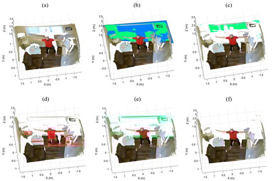
Figure 5.
The iterative plane removal of the back region: (a) the sample point cloud, (b) the verified base plane, (c,e) the verified segmented planes, (d) the invalid segmented plane, and (f) the remaining point cloud after the back wall removal.
2.5. Euclidean Clustering Removal
In this step, we cluster the remaining point cloud based on Euclidean distance to remove the irrelevant small segments and keep the objects of interest. First, we compute the Euclidean distance between each point and its neighbors. Then, we group neighboring points as a cluster if the distance between any point in an object and an adjacent point is less than a threshold cm, finishing when all the clusters are determined. Finally, we remove all small clusters with fewer than a threshold points. Figure 6 illustrates an example of Euclidean clustering removal following the iterative plane removal.
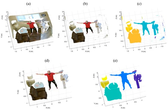
Figure 6.
Euclidean clustering on the sample point cloud (a) following the iterative plane removal (b) results in properly segmented foreground object clusters as well as residual clusters (c). Removing object clusters with fewer than μ points leaves only foreground objects (d) which can be visualized as colored objects (e).
3. Experiments and Evaluation
3.1. Experimental Setup
We evaluated our method on three generated datasets representing three different complex indoor environments, Room-1, Room-2, and Room-3, as shown in Figure 7a,c,e respectively. Each dataset contains different objects, such as furniture, planar objects, and human bodies. To measure the performance of IR-RANSAC in our challenging environments, we acquired each point cloud from an arbitrary oblique-view location using a Microsoft Kinect V2 sensor. The details of each dataset after the preprocessing steps are listed in Table 3.
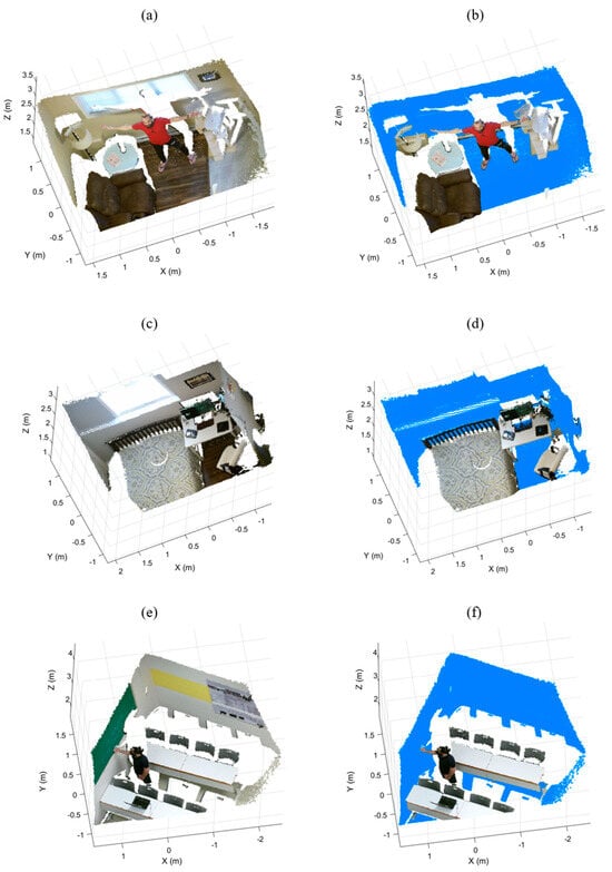
Figure 7.
The generated datasets, Room-1 (a), Room-2 (c), and Room-3 (e), and their manually labeled super-surfaces in blue (b), (d), and (f), respectively.
Table 3.
Parameters of the datasets.
To define the ground truth, we manually labeled the points belonging to each super-surface in every dataset by deploying the MATLAB Data tips tool based on their coordinates, colors, and the super-surface definition. We employed this lengthy and precise procedure by first using a semi-automated labeling approach using the orientation-based RANSAC and MATLAB Data tips tool. First, we segmented as many super-surface points as possible by running the orientation-based RANSAC in manually selected local regions known to contain super-surfaces. Then, we modified and validated the previously labeled points, resulting in the final manually labeled super-surfaces shown in Figure 7b,d,f.
We evaluated the efficiency of our IR-RANSAC and RANSAC (as a baseline) methods in terms of four pixel-based metrics: precision, recall, F1 score, and specificity. The first three parameters have been widely utilized for appraising the effectiveness of plane segmentation (e.g., [36,51,56]). To compute these metrics, we defined a true positive (TP) as a correctly identified bounding surface point, a true negative (TN) as a correctly identified foreground point, a false positive (FP) as a foreground point that was incorrectly identified as a bounding surface point, and a false negative (FN) as a bounding surface point that was incorrectly identified as a foreground point. Precision, calculated as , is the number of correctly removed points (i.e., true positives) with respect to the total number of removed points. Recall, calculated as , is the fraction of true positives among the manually labeled points (ground truth). F1 score, calculated as , or the harmonic mean of the precision and recall, represents the overall performance of our proposed method. The specificity, calculated as , reflects the true negative rate of our algorithm, providing a measure of how well our method distinguishes between foreground points and bounding surface points.
We computed the size reduction of IR-RANSAC as , where and are the sizes (i.e., the number of points) of the output point cloud and the input point cloud, respectively. We implemented our proposed algorithm using MATLAB on an Intel i5-4300M CPU @ 2.60 GHz and with 6.00 GB RAM. The full parameters of IR-RANSAC, determined through experimentation, are listed in Table 4 and were used for all our experiments.
Table 4.
Parameters of IR-RANSAC.
3.2. Experimental Results
Figure 8 shows the output results of our algorithm and the erroneously classified points for the three datasets.
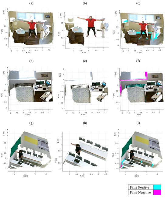
Figure 8.
Output results of IR-RANSAC. The original point clouds, Room-1 (a), Room-2 (d), and Room-3 (g), are visualized with all super-surfaces removed in (b), (e), and (h), respectively. The false positive (cyan) and false negative (magenta) points are highlighted over the original point clouds for the Room-1 (c), Room-2 (f) and Room-3 (i) datasets.
The incorrectly classified points were almost always associated with the points belonging to foreground objects that are contacting a super-surface (i.e., objects within the RANSAC distance threshold), such as the baseboard heater, the bed headboard, and the desk legs (Figure 8c,f,i respectively). Notably, as a result of our local region definitions and bounding surface criteria, we successfully prevented consideration of foreground objects that could be misidentified as bounding surfaces (e.g., beds, desks). Furthermore, foreground objects comprised of fewer points than the Euclidean clustering threshold ( points) were erroneously removed from the point cloud (e.g., the cyan portion of the lamp in Figure 8c).
Our IR-RANSAC method eliminated nearly all points belonging to the super-surfaces in the Room-1 and Room-3 datasets. However, IR-RANSAC failed to remove two small challenging regions belonging to the back and left super-surfaces in Room-2 (the magenta regions around the window and the bottom left corner of the point cloud in Figure 8f). This is because the planes surrounding the window were perpendicular to the back super-surface, and the other small plane in the bottom left corner was smaller than the verification threshold ( of the total number of points in the point cloud). Notably, both of these two misclassified regions are greater than the Euclidean clustering threshold ( points). Additionally, IR-RANSAC incorrectly assigned a small number of points belonging to foreground objects to a bounding surface. In all cases, these incorrect assignment of foreground points to super-surfaces happened in cases where the clustered foreground objects physically contacted super-surfaces (e.g., bed headboard in Figure 8f and desk legs in Figure 8i).
Figure 9 shows the output results of the standard RANSAC plane removal approach for the three datasets. The cyan and magenta colors represent the incorrectly removed regions (i.e., false positive) and undetected regions (i.e., false negative), respectively. The standard RANSAC approach failed to remove many points belonging to the super-surfaces (e.g., the back and right walls in Room-1 and the floors in the other two datasets). Moreover, RANSAC erroneously removed some parts of the human body and the furniture (e.g., couch, bed, and desks). These false segmentations have three main reasons: RANSAC’s sensitivity to clutter and occlusion, the uncertainty of RANSAC in randomly sampling three points as a minimum subset, and the lack of an orientation constraint.
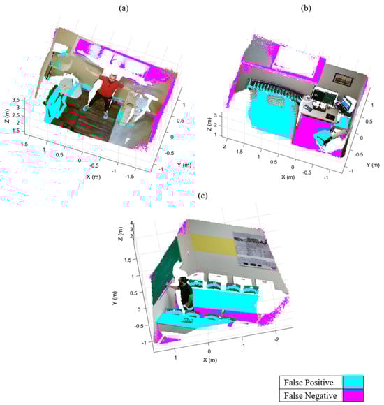
Figure 9.
The output results of standard RANSAC plane removal and its false positives and false negatives in cyan and magenta, respectively: (a) Room-1, (b) Room-2, and (c) Room-3.
Our experimental results suggest that IR-RANSAC supports varied sensor locations and removes background boundary surfaces more effectively without removing foreground data in complex 3D indoor environments.
3.3. Evaluation
Similar to RANSAC, our IR-RANSAC approach is stochastic, and accordingly its results can vary depending on the selection of the random subsample. To account for this stochasticity, we conducted 30 experiments on each dataset, similar to the work of Li et al. [39], and computed our four evaluation metrics for IR-RANSAC and standard RANSAC plane removal as a baseline comparator. We illustrate the evaluation results in Figure 10, with the left column visualizing our IR-RANSAC results and the right column representing the standard RANSAC plane removal results, and the rows corresponding to the three rooms. We implemented standard RANSAC plane removal traditionally to segment and eliminate the four largest planes in each dataset. We set the parameters of our benchmark RANSAC method to be the same as those used in IR-RANSAC. The mean (M) and standard deviation (SD) of the specificity, precision, recall, and F1 score of both approaches are shown in Table 5, along with the execution times.
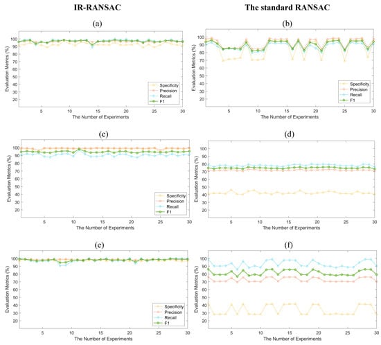
Figure 10.
The evaluation results of IR-RANSAC and standard RANSAC plane removal for the three datasets: (a) and (b) Room-1, (c) and (d) Room-2, (e) and (f) Room-3.
Table 5.
Execution times, and mean (M) and standard deviation (SD) of specificity, precision, recall, and F1 score of IR-RANSAC and standard RANSAC methods.
Given the original size of the point clouds (see Table 3), and the size of the output point clouds for Room-1 (55,705 points), Room-2 (69,044 points), and Room-3 (66,149 points), IR-RANSAC yielded a size reduction of 0.68, 0.62, and 0.64 for Room-1, Room-2, and Room-3, respectively.
4. Discussion
Our evaluation results for all four evaluation metrics achieved with IR-RANSAC (the first column of Figure 10) were higher and much more consistent than those obtained using standard RANSAC (the second column of Figure 10). Additionally, almost all four scores for IR-RANSAC had a lower standard deviation compared to those of standard RANSAC. Overall, all of our evaluation results for IR-RANSAC were statistically significantly better () than those of standard RANSAC using a two-sample t-test. Most notably, the F1 score, which represents the overall performance of the approaches, for IR-RANSAC was higher than that of standard RANSAC.
In all experiments, our proposed IR-RANSAC method obtained average values above 92% for specificity, 96% for precision, 90% for recall, and 94% for F1 score. Comparably, the standard RANSAC achieved average values between 33% and 85%, 71% and 92%, 78% and 92%, 74% and 90% for specificity, precision, recall, and F1 score, respectively. As illustrated in the second column of Figure 10, there are also many sharp fluctuations in the standard RANSAC evaluation results. The F1 score fluctuated from 82% to 95% and 76% to 86% for Room-1 and Room-3, respectively. However, it almost remained steady at 74% for the Room-2 dataset. The standard RANSAC approach demonstrated a very low specificity for Room-2 and Room-3, containing many planar furniture.
IR-RANSAC takes about three times as long to execute when compared to the standard RANSAC approach on the same datasets. This is expected though, since our IR-RANSAC method invokes the RANSAC algorithm four times more than the standard RANSAC plane removal. Theoretically, a faster version of IR-RANSAC, which has only one iteration in each local region, can be implemented that would be faster than the standard RANSAC approach because it runs the RANSAC algorithm in smaller regions.
Our evaluation results support that IR-RANSAC is a robust and reliable method for removing the bounding super-surfaces of a complex 3D indoor environment with better performance over traditional RANSAC in all ways except execution time. Our results suggest that IR-RANSAC removes background boundary surfaces effectively without removing foreground data, and can considerably reduce size of 3D point clouds.
The subjects of future research are speeding up the IR-RANSAC algorithm and improving its results in much more complex 3D indoor environments. To improve our algorithm results, we need to reduce its reliance on the Euclidean clustering technique, eliminate the small challenging regions belonging to a super-surface but with a different normal vector (e.g., the highlighted regions around the window in Figure 8f), and implement self-adaptive parameters to make the algorithm robust to different indoor environments and sensor data.
5. Conclusions
We have presented a 3D bounding surface removal technique, IR-RANSAC, that is particularly suited to more challenging and cluttered indoor environments. IR-RANSAC supports varied sensor perspectives for organized and unorganized point clouds, and it considerably reduces the size of 3D datasets. Moreover, IR-RANSAC can improve the results and the running time of different 3D computer vision methods by reducing their search space. After downsampling and denoising a point cloud captured from an oblique view, we divide the point cloud space into four overlapped local regions, exploiting knowledge of the current view of the sensor, and segment a base plane in each of the four regions. We then expand our search space around the base plane in each region, and iteratively segment and remove the remaining points belonging to each super-surface. Finally, we cluster the remaining point cloud using the geometric relationship between groups of points, resulting in a final point cloud comprised only of clustered objects of interest. We evaluated the performance of IR-RANSAC in terms of four metrics: specificity, precision, recall, and F1 score, on the three generated datasets acquired from an arbitrary oblique-view location and representing different indoor environments. Our experiments demonstrated that our proposed method is a robust super-surface removal and size reduction technique for complex 3D indoor environments. Experimentally, IR-RANSAC outperformed traditional RANSAC segmentation in all categories, supporting our efforts to prioritize the inclusion of all bounding points in each super-surface, while minimizing inclusion of points that belong to foreground objects.
Our intention was to develop a robust method of bounding surface segmentation—maximizing inclusion of bounding surface points and minimizing inclusion of foreground points. Our experimental data suggest that by conceptualizing bounding surfaces (e.g., walls and floor) as unique and different than other large surfaces that belong to foreground objects, it is possible to improve on methods of segmenting and removing these unwanted bounding surfaces specifically. By removing these bounding surfaces and preserving foreground objects, we considerably reduce the size of the resulting dataset, substantially improving downstream storage and processing.
Author Contributions
A.E. developed the method, collected results, and drafted and revised the paper. S.C. conceived of the study and contributed to the analysis and revisions. Both authors have read and agreed to the published version of the manuscript.
Funding
This work was supported by the Natural Sciences and Engineering Research Council of Canada under grant number RGPIN-2016-04165.
Institutional Review Board Statement
Ethical review and approval were not required for this study because all data were collected from members of the research team.
Informed Consent Statement
Patient consent was waived because all data were collected from members of the research team.
Data Availability Statement
The data presented in this study are available on request from the corresponding author. The data are not publicly available at the time of publication due to insufficient resources for making the data publicly accessible.
Conflicts of Interest
The authors declare no conflict of interest. The funders had no role in the design of the study; in the collection, analyses, or interpretation of data; in the writing of the manuscript, or in the decision to publish the results.
References
- Shaikh, S.H.; Saeed, K.; Chaki, N. Moving object detection using background subtraction. In SpringerBriefs in Computer Science; Springer: Berlin, Germany, 2014; pp. 15–23. [Google Scholar]
- Kumar, S.; Yadav, J.S. Video object extraction and its tracking using background subtraction in complex environments. Perspect. Sci. 2016, 8, 317–322. [Google Scholar] [CrossRef]
- Aggarwal, A.; Biswas, S.; Singh, S.; Sural, S.; Majumdar, A.K. Object tracking using background subtraction and motion estimation in MPEG videos. In Lecture Notes in Computer Science; (Including Subseries Lecture Notes in Artificial Intelligence and Lecture Notes in Bioinformatics); Springer: Berlin, Germany, 2006; Volume 3852 LNCS, pp. 121–130. [Google Scholar] [CrossRef]
- Manikandan, R.; Ramakrishnan, R.; Scholar, R. Human Object Detection and Tracking using Background Subtraction for Sports Applications. Int. J. Adv. Res. Comput. Commun. Eng. 2013, 2, 4077–4080. Available online: https://www.researchgate.net/publication/276903638 (accessed on 23 October 2020).
- Czarnuch, S.; Cohen, S.; Parameswaran, V.; Mihailidis, A. A real-world deployment of the COACH prompting system. J. Ambient Intell. Smart Environ. 2013, 5, 463–478. [Google Scholar] [CrossRef]
- Zou, W.; Lu, Y.; Chen, M.; Lv, F. Rapid face detection in static video using background subtraction. In Proceedings of the 2014 10th International Conference on Computational Intelligence and Security, CIS 2014, Kunming, China, 15–16 November 2014; pp. 252–255. [Google Scholar] [CrossRef]
- Yang, H.; Qu, S. Real-time vehicle detection and counting in complex traffic scenes using background subtraction model with low-rank decomposition. IET Intell. Transp. Syst. 2018, 12, 75–85. [Google Scholar] [CrossRef]
- Sahu, A.K.; Choubey, A. Motion Detection Surveillance System Using Background Subtraction Algorithm. Int. J. Adv. Res. Comput. Sci. Manag. Stud. 2013, 1, 58–65. Available online: www.ijarcsms.com (accessed on 23 October 2020).
- Hargude, S.; Idate, S.R. I-Surveillance: Intelligent Surveillance System Using Background Subtraction Technique. In Proceedings of the 2nd International Conference on Computing, Communication, Control and Automation, ICCUBEA 2016, Pune, India, 12–13 August 2016. [Google Scholar] [CrossRef]
- Karaman, M.; Goldmann, L.P. Comparison of Static Background Segmentation Methods, spiedigitallibrary.org. 2005. Available online: https://www.spiedigitallibrary.org/conference-proceedings-of-spie/5960/596069/Comparison-of-static-background-segmentation-methods/10.1117/12.633437.short (accessed on 23 October 2020).
- Stauffer, C.; Grimson, W.E.L. Adaptive background mixture models for real-time tracking. Proc. IEEE Comput. Soc. Conf. Comput. Vis. Pattern Recognit. 1999, 2, 246–252. [Google Scholar] [CrossRef]
- Zivkovic, Z. Improved adaptive Gaussian mixture model for background subtraction. In Proceedings of the International Conference on Pattern Recognition, Cambridge, UK, 26 August 2004; Volume 2, pp. 28–31. [Google Scholar] [CrossRef]
- Kim, K.; Chalidabhongse, T.H.; Harwood, D.; Davis, L. Real-time foreground-background segmentation using codebook model. Real-Time Imag. 2005, 11, 172–185. [Google Scholar] [CrossRef]
- Guo, J.M.; Liu, Y.F.; Hsia, C.H.; Shih, M.H.; Hsu, C.S. Hierarchical method for foreground detection using codebook model. IEEE Trans. Circuits Syst. Video Technol. 2011, 21, 804–815. [Google Scholar] [CrossRef]
- Tsai, D.M.; Lai, S.C. Independent component analysis-based background subtraction for indoor surveillance. IEEE Trans. Image Process. 2009, 18, 158–167. [Google Scholar] [CrossRef]
- Jiménez-Hernández, H. Background Subtraction Approach Based on Independent Component Analysis. Sensors 2010, 10, 6092–6114. [Google Scholar] [CrossRef]
- Gordon, G.; Darrell, T.; Harville, M.; Woodfill, J. Background estimation and removal based on range and color. In Proceedings of the 1999 IEEE Computer Society Conference on Computer Vision and Pattern Recognition, Fort Collins, CO, USA, 23–25 June 1999; Volume 2, pp. 459–464. [Google Scholar] [CrossRef]
- Czarnuch, S.; Mihailidis, A. Development and evaluation of a hand tracker using depth images captured from an overhead perspective. In Disability and Rehabilitation: Assistive Technology; Taylor and Francis Ltd.: Abingdon, UK, 2016; Volume 11, pp. 150–157. [Google Scholar] [CrossRef][Green Version]
- Shotton, J.; FitzGibbon, A.; Cook, M.; Sharp, T.; Finocchio, M.; Moore, R.; Kipman, A.; Blake, A. Real-time human pose recognition in parts from single depth images. In Proceedings of the IEEE Computer Society Conference on Computer Vision and Pattern Recognition, Washington, DC, USA, 20–25 June 2011; pp. 1297–1304. [Google Scholar] [CrossRef]
- Kolmogorov, V.; Criminisi, A.; Blake, A.; Cross, G.; Rother, C. Bi-layer segmentation of binocular stereo video. In Proceedings of the 2005 IEEE Computer Society Conference on Computer Vision and Pattern Recognition, CVPR 2005, San Diego, CA, USA, 20–26 June 2005; Volume II; pp. 407–414. [Google Scholar] [CrossRef]
- Fernandez-Sanchez, E.J.; Diaz, J.; Ros, E. Background subtraction based on color and depth using active sensors. Sensors 2013, 13, 8895–8915. [Google Scholar] [CrossRef] [PubMed]
- Cristani, M.; Farenzena, M.; Bloisi, D.; Murino, V. Background subtraction for automated multisensor surveillance: A comprehensive review. EURASIP J. Adv. Signal. Process. 2010, 2010. [Google Scholar] [CrossRef]
- Zhou, W.; Yuan, J.; Lei, J.; Luo, T. TSNet: Three-stream Self-attention Network for RGB-D Indoor Semantic Segmentation. IEEE Intell. Syst. 2020, 1672. [Google Scholar] [CrossRef]
- Ottonelli, S.; Spagnolo, P.; Mazzeo, P.L.; Leo, M. Improved video segmentation with color and depth using a stereo camera. In Proceedings of the 2013 IEEE International Conference on Industrial Technology (ICIT), Cape Town, South Africa, 25–28 February 2013; pp. 1134–1139. [Google Scholar] [CrossRef]
- The Point Cloud Libraryle. Available online: https://pointclouds.org/ (accessed on 10 December 2020).
- Muthu, S.; Tennakoon, R.; Rathnayake, T.; Hoseinnezhad, R.; Suter, D.; Bab-Hadiashar, A. Motion Segmentation of RGB-D Sequences: Combining Semantic and Motion Information Using Statistical Inference. IEEE Trans. Image Process. 2020, 29, 5557–5570. [Google Scholar] [CrossRef] [PubMed]
- Vaskevicius, N.; Birk, A.; Pathak, K.; Schwertfeger, S. Efficient representation in three-dimensional environment modeling for planetary robotic exploration. Adv. Robot. 2010, 24, 1169–1197. [Google Scholar] [CrossRef]
- Czerniawski, T.; Nahangi, M.; Walbridge, S.; Haas, C. Automated removal of planar clutter from 3D point clouds for improving industrial object recognition. In Proceedings of the ISARC 2016—33rd International Symposium for Automation and Robotics, Construction, Auburn, AL, USA, 18–21 July 2016; pp. 357–365. [Google Scholar] [CrossRef]
- Kaushik, R.; Xiao, J. Accelerated patch-based planar clustering of noisy range images in indoor environments for robot mapping. Rob. Auton. Syst. 2012, 60, 584–598. [Google Scholar] [CrossRef]
- Zhang, C. Perspective Independent Ground Plane Estimation by 2D and 3D Data Analysis, ieeexplore.ieee.org. 2020. Available online: https://ieeexplore.ieee.org/abstract/document/9081938/ (accessed on 19 January 2021).
- Chen, S.; Tian, D.; Feng, C.; Vetro, A.; Kovačević, J. Fast resampling of three-dimensional point clouds via graphs. IEEE Trans. Signal. Process. 2018, 66, 666–681. [Google Scholar] [CrossRef]
- Fischler, M.A.; Bolles, R.C. Random sample consensus: A Paradigm for Model Fitting with Applications to Image Analysis and Automated Cartography. Commun. ACM 1981. [Google Scholar] [CrossRef]
- Ballard, D.H. Generalizing the Hough transform to detect arbitrary shapes. Pattern Recognit. 1981, 13, 111–122. [Google Scholar] [CrossRef]
- Vosselman, G.; Sithole, G.; Vosselman, G.; Gorte, B.G.H.; Sithole, G.; Rabbani, T. Recognising Structure in Laser Scanner Point Clouds. Int. Arch. Photogramm. Remote Sens. Spat. Inf. Sci. 2004, 46, 33–38. [Google Scholar]
- Borrmann, D.; Elseberg, J.; Lingemann, K.; Nüchter, A. The 3D Hough Transform for plane detection in point clouds: A review and a new accumulator design. 3D Res. 2011, 2, 1–13. [Google Scholar] [CrossRef]
- Vo, A.V.; Truong-Hong, L.; Laefer, D.F.; Bertolotto, M. Octree-based region growing for point cloud segmentation. ISPRS J. Photogramm. Remote Sens. 2015, 104, 88–100. [Google Scholar] [CrossRef]
- Awwad, T.M.; Zhu, Q.; Du, Z.; Zhang, Y. An improved segmentation approach for planar surfaces from unstructured 3D point clouds. Photogramm. Rec. 2010, 25, 5–23. [Google Scholar] [CrossRef]
- Chen, D.; Zhang, L.; Mathiopoulos, P.T.; Huang, X. A methodology for automated segmentation and reconstruction of urban 3-D buildings from ALS point clouds. IEEE J. Sel. Top. Appl. Earth Obs. Remote Sens. 2014, 7, 4199–4217. [Google Scholar] [CrossRef]
- Li, L.; Yang, F.; Zhu, H.; Li, D.; Li, Y.; Tang, L. An improved RANSAC for 3D point cloud plane segmentation based on normal distribution transformation cells. Remote Sens. 2017, 9, 433. [Google Scholar] [CrossRef]
- Tarsha-Kurdi, F.; Landes, T.; Grussenmeyer, P. Hough-Transform and Extended Ransac Algorithms for Automatic Detection of 3D Building Roof Planes From Lidar Data. In Proceedings of the ISPRS Workshop Laser Scanning 2007 SilviLaser 2007, Espoo, Finland, 12–14 September 2007; Volume XXXVI, pp. 407–412. [Google Scholar]
- Tóvári, D.; Pfeifer, N. Segmentation based robust interpolation—A newapproach to laser data filtering. Int. Arch. Photogramm. Remote Sens. Spat. Inf. Sci. ISPRS Arch. 2005, 36, 79–84. [Google Scholar]
- Nurunnabi, A.; Belton, D.; West, G. Robust segmentation in laser scanning 3D point cloud data. In Proceedings of the 2012 International Conference on Digital Image Computing Techniques and Applications, DICTA 2012, Fremantle, WA, Australia, 3–5 December 2012; pp. 1–8. [Google Scholar] [CrossRef]
- Deschaud, J.-E.; Goulette, F. A Fast and Accurate Plane Detection Algorithm for Large Noisy Point Clouds Using Filtered Normals and Voxel Growing. 2010. Available online: https://hal-mines-paristech.archives-ouvertes.fr/hal-01097361 (accessed on 5 December 2020).
- Huang, M.; Wei, P.; Liu, X. An Efficient Encoding Voxel-Based Segmentation (EVBS) Algorithm Based on Fast Adjacent Voxel Search for Point Cloud Plane Segmentation. Remote Sens. 2019, 11, 2727. [Google Scholar] [CrossRef]
- Xiao, J.; Zhang, J.; Adler, B.; Zhang, H.; Zhang, J. Three-dimensional point cloud plane segmentation in both structured and unstructured environments. Rob. Auton. Syst. 2013, 61, 1641–1652. [Google Scholar] [CrossRef]
- Leng, X.; Xiao, J.; Wang, Y. A multi-scale plane-detection method based on the Hough transform and region growing. Photogramm. Rec. 2016, 31, 166–192. [Google Scholar] [CrossRef]
- Teboul, O.; Simon, L.; Koutsourakis, P.; Paragios, N. Segmentation of building facades using procedural shape priors. In Proceedings of the IEEE Computer Society Conference on Computer Vision and Pattern Recognition, San Francisco, CA, USA, 13–18 June 2010; pp. 3105–3112. [Google Scholar] [CrossRef]
- Filin, S. Surface clustering from airborne laser scanning data. In Proceedings of the International Archives of the Photogrammetry, Remote Sensing and Spatial Information Sciences, Denver, CO, USA, 10–15 November 2002; pp. 119–124. [Google Scholar]
- Filin, S.; Pfeifer, N. Segmentation of airborne laser scanning data using a slope adaptive neighborhood. ISPRS J. Photogramm. Remote Sens. 2005, 60, 71–80. [Google Scholar] [CrossRef]
- Zhou, G.; Cao, S.; Zhou, J. Planar Segmentation Using Range Images From Terres-trial Laser Scanning. IEEE Geosci. Remote Sens. Lett. 2016, 13, 257–261. [Google Scholar] [CrossRef]
- Dong, Z.; Yang, B.; Hu, P.; Scherer, S. An efficient global energy optimization approach for robust 3D plane segmentation of point clouds. ISPRS J. Photogramm. Remote Sens. 2018, 137, 112–133. [Google Scholar] [CrossRef]
- Pomerleau, F.; Colas, F.; Siegwart, R.; Magnenat, S. Comparing ICP variants on real-world data sets. Auton. Robot. 2013. [Google Scholar] [CrossRef]
- Rusu, R.B.; Cousins, S. 3D is here: Point Cloud Library (PCL). In Proceedings of the IEEE International Conference on Robotics and Automation, Shanghai, China, 9–13 May 2011. [Google Scholar] [CrossRef]
- Rusu, R.B.; Marton, Z.C.; Blodow, N.; Dolha, M.; Beetz, M. Towards 3D Point cloud based object maps for household environments. Rob. Auton. Syst. 2008, 56, 927–941. [Google Scholar] [CrossRef]
- Förstner, W.; Wrobel, B.P. Photogrammetric Computer Vision; Springer: Berlin, Germany, 2016. [Google Scholar]
- Yan, J.; Shan, J.; Jiang, W. A global optimization approach to roof segmentation from airborne lidar point clouds. ISPRS J. Photogramm. Remote Sens. 2014, 94, 183–193. [Google Scholar] [CrossRef]
Publisher’s Note: MDPI stays neutral with regard to jurisdictional claims in published maps and institutional affiliations. |
© 2021 by the authors. Licensee MDPI, Basel, Switzerland. This article is an open access article distributed under the terms and conditions of the Creative Commons Attribution (CC BY) license (https://creativecommons.org/licenses/by/4.0/).