1. Introduction
An IMU (Inertial Measurement Unit) consists of tri-axial accelerometers, tri-axial gyroscopes and sometimes tri-axial magnetometers. A lot of research has been done about IMUs in fields of aerospace, navigation and robotics for several years. This is because of some unique and beneficial characteristics (compare, e.g., Reference [
1] or Reference [
2])—high temporal resolution, orientation estimation, high short term accuracy and unlimited availability independent from exterior environment.
In the early beginnings of IMU technology it was both rather expensive and unhandy in size [
3]. Size, cost and power consumption have been dramatically reduced due to recent developments of MEMS (Microelectromechanical systems) [
4]. This led to an even broader scope of applications and accelerated research [
3].
Initially mainly used in navigation tasks, IMUs are now used in several applications for example, Augmented Reality, Indoor- and Smartphone navigation, Robotics and Mobile Mapping Systems. MEMS IMUs in particular are nowadays not only used for mobile mapping and navigation tasks by the geodetic community. Due to its unlimited measuring range compared to conventional inclination sensors, accelerometer horizon leveling attracted interest. Accelerometer horizon leveling means computation of two angles roll
and pitch
making use of accelerometer triads sensing the local gravity vector. In the following we use the term leveling instead of horizon leveling for the purpose of readability—not to be confused with leveling as a method for determination of height differences. Lately, accelerometer leveling has been used for deformation monitoring [
5,
6] and frequency analysis of vibrations, for example, References [
7,
8].
Another usecase of leveling with MEMS IMUs is tilt compensation of GNSS (Global Navigation Satellite System) poles, see Reference [
9] or Reference [
10]. Generally leveling is used in navigation and pose estimation during unaccelerated phases to stabilize attitude and to compensate gyroscope drifts. These direct measurements of the two tilt angles
and
are fed into IMU strapdown computation or a Kalman Filter for sensor fusion.
In Engineering Geodesy it is very often required to manually align instruments, sensors or measurement equipment with the local vertical defined by gravity. For 3D-point-measurements using a total station and a pole mounted prism, both need to be leveled using a circular level accurate to 6 arc minutes (see e.g., Reference [
11]). Six arc minutes correspond to 2.6 mm horizontal position error at a height of 1.5 m. Modern total stations use liquid based tilt compensators to correct residual tilts. These sensors have inert measurement properties and a very limited measuring range [
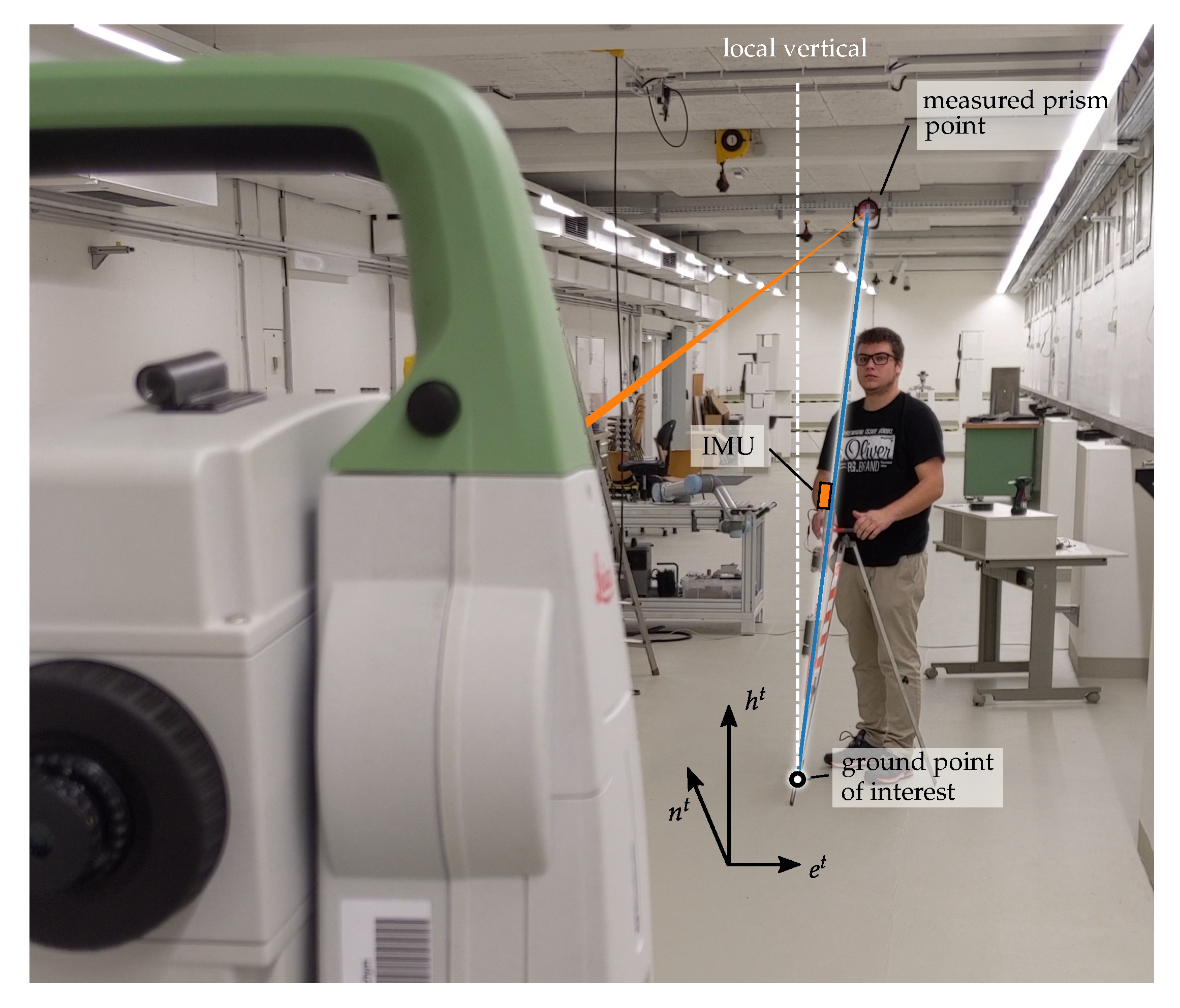
12]. For a prism pole no residual tilt correction sensor is available and errors up to 3 mm are easily introduced. Furthermore the leveling of a pole is the most time consuming part of measuring 3D-point-coordinates. The novel idea in this contribution is to bring the concept of IMU based leveling to the prism pole (see
Figure 1), similar to what Reference [
9] did for a GNSS pole. Advanced requirements on the accuracy of pole tilt compensation arise with the increased accuracy of a total station compared to GNSS. In this contribution we show how a calibration for such a system can be performed and we analyze which parameters are important. The accelerometer triad sensor models have to cope with the advanced accuracy demands. Extensive research has been carried out in the scientific community concerning IMU sensor models. The choice of the inertial instrument error model depends on the application/use-case and on the effect on the derived quantities [
13] (p. 574f). Two basic categories of calibration approaches are distinguished: online and pre-calibration. In the first approach, parameters of the IMU error model (see
Section 2.1) are estimated in real time using sensor fusion (e.g., Kalman Filter) with external observations, for example, GNSS-IMU integration. The deterministic observability of such state parameters depends on the user dynamics [
13] (p. 574f) and is not applicable in static applications. In addition, pre-calibration should be preferred, due to the higher noise level of MEMS sensors, since
the possibilities to reduce noise in static environment through time-averaging, and
the danger of vibrations overlaying systematics in kinematic applications.
Nevertheless, at least sensor biases should always be estimated online, since these parameters highly depend on temperature and might change significantly over time [
14,
15].
Two groups of pre-calibration methods referring to calibration setup can be found in literature. The first depends on additional equipment like a reference sensor (e.g., aviation grade IMU, rate tables [
16,
17,
18,
19], or optical 6DoF-tracking [
20]) and is supposed to be executed in the laboratory. Such high precision equipment is expensive or might not be available [
21] and is not economical for low-cost MEMS sensors [
22]. We summarize these approaches as equipment-aided calibrations.
The other group of approaches targets suitable methods for in-field calibration. These methods mostly rely on gravity and should be feasible for end users. Reference [
23] first introduced the accelerometer calibration using the property—the magnitude of the static acceleration measured must equal that of the gravity. This group is referred to as gravity-based approaches. Methods based on this property have in common, that gravity (
) is measured in multiple quasi-static positions (attitudes). Extensive research has been carried out, differing in number of positions and the underlying estimated error models. A summary can be found in
Table 1.
In this contribution we investigate different accelerometer triad error models utilizing a 6-joints industrial robot. In order to compensate the pole tilt, additional mounting parameters of the triad w.r.t. the pole need to be estimated.
The remainder of this paper is organized as follows. In
Section 2 we describe the various models of accelerometer triads, gravity-based leveling and pole tilt compensation. In the following
Section 3, we show how the triad model parameters are calibrated and how the mounting parameters are estimated. In
Section 4 we investigate calibration and mounting parameters concerning their contribution to the uncertainty of the final tilt compensation. Here variance based sensitivity analysis is used to identify and improve important parameters. The results of the calibration and a final evaluation experiment are presented in
Section 5, whereas
Section 6 concludes this contribution.
2. Methodology
To reduce the measured prism to the ground point for a tilted pole, it is necessary to know the orientation of the pole. This involves several coordinate frames (compare
Figure 1 and
Figure 2) accumulating in the transformation from pole frame
to the
local geodetic frame (the frame of total station measurements). First we define the coordinate system of the pole (
pole frame denoted by
) so that the origin is placed at the prism,
points downwards to the tip,
lies in the plane defined by the IMU axis
and
;
completes the right-handed coordinate system. The sensitive axes of the 3 accelerometers form the
sensor frame denoted by
. The calibrated forces of the accelerometer triad refer to the
body frame (
) of the IMU. The process of leveling determines the rotation of the
body frame w.r.t. the local
navigation frame (aligned with local vertical) denoted by
.
Making use of these frames, pole tilt compensation involves three main computation steps:
Application of an appropriate tri-axis accelerometers sensor model to derive calibrated specific force measurements, which is in fact transformatoion from
s-frame to
b-frame. (
Section 2.1)
In unaccelerated motion the sensed earth gravity can be used to compute roll and pitch attitudes w.r.t. the n-frame.
In combination with an externally estimated yaw angle, the pole length and the mounting parameters, the components of the askew pole w.r.t. the t-frame is computed.
2.1. Sensor Models
Several sensor models can be found in literature. They differ mainly in the modeled error parameters. The basic model for the measured accelerometer outputs (measured forces) denoted by
proposed by Reference [
23] is:
where
is the calibrated force vector,
is the offset or biases vector and
is the scale factor diagonal matrix and
is the accelerometer random noise.
The calibrated forces
refer to the three accelerometer sensitivity axes, thus denoted by
. Ideally these axes should be orthogonal, but due to imprecise manufacturing this is most likely not the case. Therefore, Reference [
16] extended their model to account for this non-orthogonality of the sensor sensitivity axis by introducing
which transforms the sensitivity axes to the orthogonal body or IMU-frame (denoted by
) by use of 6 parameters. Here these parameters can be interpreted as
small angles, where
is the rotation of the
i-th axis around the
j-th body axis, compare
Figure 3. If both rotations about one axis are equal, for example,
for all rotation axes, Equation (
3) becomes a skew-symmetric matrix, which corresponds to the well known small angle approximation rotation matrix.
Defining the body frame so that
x-axes coincide and
-axis lies in the plane spanned by
and
Equation (
3) reduces to (compare
Figure 3):
This gives a 9-parameter model by extending Equation (
1) with Equation (
4) comprising three additional non-orthogonality parameters
:
2.2. Leveling
Following equations are used for accelerometer leveling [
13], which describe the orientation of the IMU body frame
with respect to the local navigation frame denoted by
. Euler angles are used to describe the attitude using roll
, pitch
and yaw
rotations.
Note that arctan2() must be used for roll computation, but if limiting tilting to the upper half sphere it can be replaced by arctan().
The accuracy of this leveling process depends on the model parameters for accelerations and accelerations noise. For example, a 1 mrad roll and pitch accuracy is obtained from accelerometers accurate to
g. However, disturbing motions such as vibrations or human activity influences the leveling process. In case this motion averages out over time, its effects may be reduced simply by time-averaging [
13]. This is applied in all experiments in the remainder of this contribution, since human shaking during pole handling is relevant for the application regarded in this case. Furthermore one has to consider present auto-correlation and cross-correlation in the specific force measurement data.
2.3. Pole Tilt Compensation
For coherent pole tilt compensation it is necessary to know the exact relation between the IMU
b-frame and the poles
p-frame. The IMU is placed somewhere on the pole rotated by the Euler angles
which define the rotation from
b-frame to
p-frame (see
Figure 2). These angles can be converted to a rotation matrix or coordinate transformation matrix
:
where the definition of rotation axes and rotation sequence is shown in
Appendix A. The pole length
is the distance from prism center to the pole tip and can be expressed in pole coordinates as:
With the rotation of the pole frame to the local horizontal navigation frame (
) defined by
or
, the tilted pole can be converted to horizontal
n-frame by (see also
Figure 2):
where
must be determined from heading estimation,
is computed by accelerometer leveling and
describes the mounting and needs to be calibrated. For the notation using parentheses, please refer to
Appendix A. The resulting
then describes the coordinate components of the tilted pole w.r.t. the
n-frame.
Finally the coordinates of the pole tip
(= the ground point) are computed from the measured prism point
:
where
takes care of converting the
n-frame to the local geodetic frame (
). The frames
p,
b,
n are designed as NED-system, while the
t-frame (= the total station system) is usually an ENU-system.
3. Calibration Procedure
The proposed calibration procedure here consists of two parts.
The first part involves a 6-joints industrial robot arm, holding the IMU under consideration to perform the tri-axial
accelerometer calibration, referring to the sensor models in
Section 2.1.
In the second part a total station is used to estimate the mounting parameters
introduced in Equation (
7),
Section 2.3. We call this sub-procedure
mounting estimation.
For the first, the method is described in
Section 3.1 to estimate the parameters of various sensor models introduced in
Section 2.1. We investigate different subsets of parameters in Equation (
5) giving the following models (denoted by
) listed below:
These are estimated using the 24 position scheme proposed by Reference [
26], see
Section 3.1. For the mounting estimation, the IMU is mounted on a prism pole and the prism is tracked by a total station. By tilting the pole in different directions over a known ground point the mounting parameters are determined. The method is described in
Section 3.2.
3.1. Accelerometers Calibration
The
gravity-based approach uses the fact, that the norm of measured gravity must be independent from attitude of the IMU under quasi-static conditions [
23]. As long as the position displacement does not exceed a certain limit the length of
is constant. Apart from local gravity variation a change in longitude has no effect, a change in latitude means about 1 mm s
−2 per 55
. Theoretically the norm of the measured specific force must equal the norm of the gravity:
The disadvantage of these approaches is, that
must be known. Generally, no exact measurement of
is available, but values from theoretical models can be computed. Anyhow for applications exclusively concerned about leveling the length of
does not matter, hence a length of 1 could have been used [
29].
Model (
12) can be used as the functional part of a Gauss-Helmert-Adjustment (GH) to estimate the different model parameters of the tri-axial accelerometers of Equation (
5) by replacing
with the corresponding model by inverting Equation (
5). The scale matrix
is easily invertible, since it is a diagonal matrix. For the application of Equation (
5) it is also necessary, that
is invertible, which is given by the fact, that triangular matrices are invertible if all diagonal elements are non-zero, which is the case for
. This is then solved using the well-known iterative nonlinear least squares algorithm, cf. Reference [
30]. Since 9 parameters are to be estimated in Equation (
5), at least 9 positions (=9 condition equations like (
5)) are required [
17]. However, a more sophisticated calibration scheme is necessary for reliable estimates of the parameters. Reference [
26] proposed a 24-position scheme consisting of eight 50 gon rotations per accelerometer axis. This scheme distributes the measured
-vector evenly over the unit-sphere. The stochastic model is then made up of a block diagonal matrix
, consisting of
n (=number of positions) 3 × 3 matrices
empirically determined. This is done by estimating the variance covariance matrix (VCM) using approx. 250 measurements during each stable position. Afterwards the variance of the mean is computed, since the epochs have been proven uncorrelated during auto-correlation investigations.
From a practical point of view, this calibration approach is also applicable in the field, without additional equipment and data collection can be done by hand. Others have used rotation tables or polyhedrons for IMU placement. In this contribution we use a 6-joints industrial robot arm as IMU carrier. This has some advantages: unlimited spectrum of possible attitudes, accurate reproducibility and time efficiency, since no human interaction is necessary.
3.2. Mounting Calibration
To estimate the mounting of the IMU on the pole, that is the rotation
between the pole system (
p-frame) and IMU system (
b-frame) we tilt the pole with the tip fixed on a coordinatively known ground point
. Starting from Equation (
10) the following condition must hold:
Denoting
by
describing pole components measured by the total station, and
as pole components measured by IMU, the condition can be rewritten as:
To get rid of the additional yaw parameter
in Equation (
9), we consider only horizontal displacement
of the prism. Then condition, Equation (
14) reduces to:
This way the attitude of the IMU
reduces to the leveling parameters
, while the mounting parameters
already only consist of
because of the frame definitions described in
Section 2. With Equation (
15), the following condition equation can be defined for every prism position:
The parameters in this model are the roll
and pitch
from
p-frame to
b-frame. The east
and north
coordinates of the prism, measured by the total station form the observation vector together with the IMU accelerometer readings
. We have also designed the ground point (
) as observations to account for the small gliding or moving of the pole tip while tilting the pole. The pole length
is considered a non-stochastic quantity in this model. The pole is held static for a period of about 5 to 10 s using a three-legged clamp (see
Section 5). A scheme of 40 positions with tilts of up to 50 gon is performed.
One can think of combining mounting estimation and accelerometer calibration into one single adjustment by replacing
in Equation (
16) with the according sensor model, for example, Equation (
5). In theory, that would be the preferable approach. We have decided to split these two adjustments, because from a practical point of view, it is only possible to tilt the pole over a known ground point up to about 50 gon, whereas for the accelerometer calibration it is necessary to have rotations all over the sphere.
4. Variance Based Sensitivity Analysis
Variance based sensitivity analysis (VBSA) can be used to analyze the relations between input and output parameters of a model. The goals of sensitivity analysis are listed in References [
31,
32]:
This concept was brought to the engineering geodesy context by References [
32,
33] and has been used in many studies since then (e.g., References [
34,
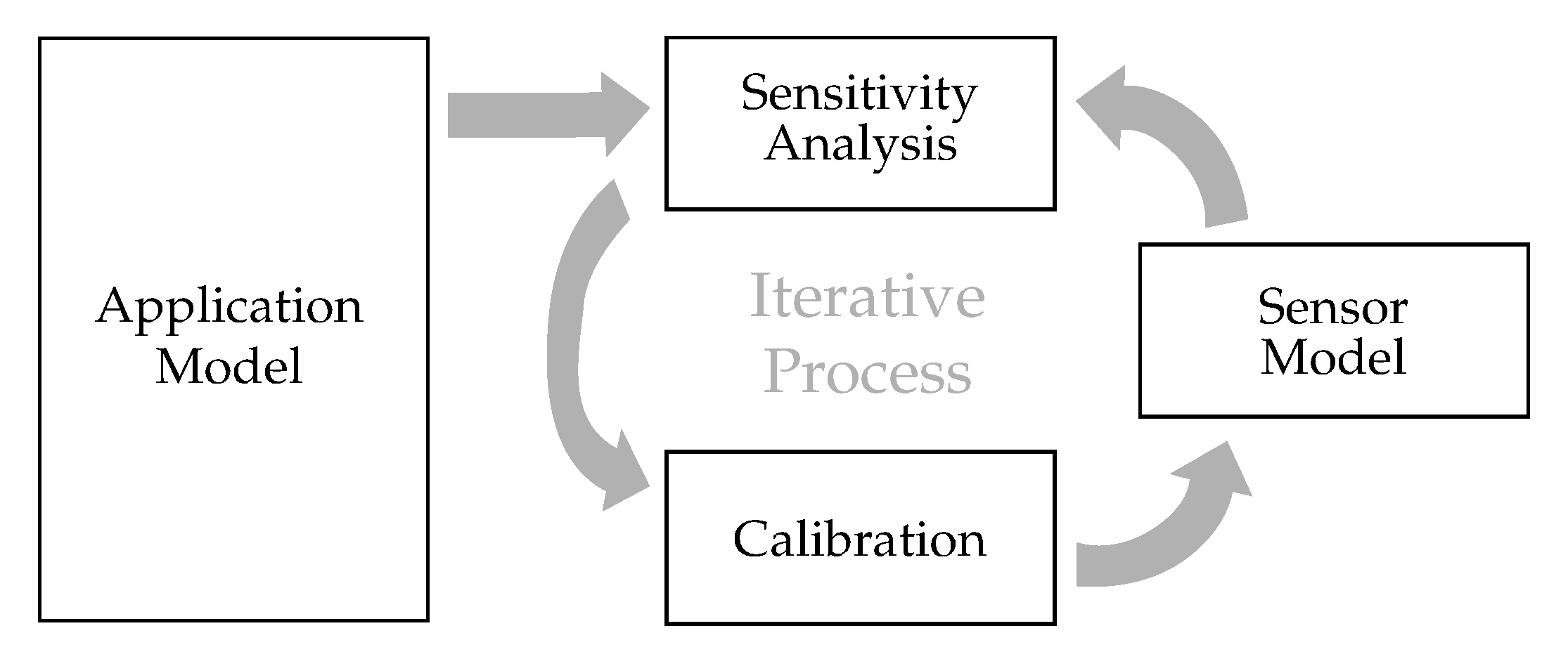
35]). Please refer to these references for details of the methodology and implementation. In this contribution VBSA is a powerful tool to analyze and optimize the calibration process under consideration of the target application. The basic idea is shown in
Figure 4.
The sensor model is already given in
Section 2.1 (
5):
which connects sensed specific forces
to calibrated specific forces
through the calibration parameters
(based on the model
,
Section 3). It is not clear from the first sight, which calibration parameters are important for specific applications, in our case
leveling or
pole tilt compensation. For this purpose we investigate the influence of the calibration parameters on the outputs of the following application models:
The goal is to improve the calibration configuration in an efficient way to improve the output parameters of the application model in a sense of reduced variance. Our approach first analyzes the contribution of each input quantity on the output variance of the application model under consideration, for example, roll and pitch of model
. This can be done utilizing VBSA, computing the
total effect for the
i-th input measure, for example,
on the
j-th element of
by:
Here
describes the variance of the output parameter and
describes the output variance that one would end up with if all other quantities except
could be known or fixed. The total effect terms are computed using a special sample scheme for the correct generation (=simulation) of the conditional variances using the original nonlinear models. The simulation and analysis of correlated input is not considered so far. Sensitivity analysis for leveling is shown in
Section 4.1. The calibration parameter with the highest effect is the one to be improved. A method to improve the calibration configuration for a GH-estimation of the calibration parameters taking these aspects into account is shown in
Section 4.2. This is an iterative process, that can be repeated until the desired output variance of the application model is reached. This section is concluded by the sensitivity analysis of the pole tilt compensation (
Section 4.3).
4.1. Leveling
The total effect terms of the IMU sensor model parameters on the leveling output quantities Equation (
18)
are shown in
Figure 5. The computation is based on the results of the IMU Calibration
(see
Section 5.1) and a
of 30 mm s
−2 from empirical investigations of the IMU in use. This corresponds to a root noise density
of 4.2 mg/
. Time averaging of forces over
uncorrelated epochs is also considered. The theoretical standard deviation of tilt angles
from variance-covariance propagation is about 160 mgon with variations of ±3 mgon. The analysis is done for 5 classes, depending on the tilting and the resulting prism displacement.
represents the approximately leveled case,
results from a tilt of about 20 gon (=40 cm prism displacement) from vertical and
to
are tilted about 40 gon (=80 cm) in different directions. We have included only displacements for one quadrant, since we know from previous studies, that the influences are perfectly symmetric [
36].
The following conclusions can be derived:
For this IMU specifications, the raw observations make up about half of the output tilt variances with a small dependence on prism displacement.
For smaller tilt angles < 30 [gon] z-accelerometer reading is inessential for both tilt angles, whilst y-accelerometer is dominant for roll and x-accelerometer is dominant for pitch computation. This makes sense, considering the corresponding rotation axes of the rotation angles (x for and y for ).
Contribution of z-accelerometer readings increase with prism displacement (or tilt respectively) (compare , with , , )
Concerning the calibration parameters, both bias and scale parameters have very low influence on the resulting parameter variance, whereas
has a big share on the variance of
and
on
. This is plausible, since for example,
nearly directly distort roll
, since both are rotations about the
x-axis, compare
Figure 3.
Whilst we have no influence on the IMU specification from a methodogical point of view, except of buying a better one, we can focus on the two non-orthogonality parameters to improve leveling performance, which cause up to almost 50% of the leveling uncertainty.
4.2. Improvement Strategy
With this conclusions from VBSA one can ask for an optimal or improved accelerometer calibration configuration. But not with the goal to improve the overall result (by means of minimal variance of all the parameters), instead search for a configuration to improve the most relevant parameters for the specific application, namely the non-orthogonality parameters
identified before in
Section 4.1. Practically this means searching for calibration positions (in fact = pose), that maximize the sensitivity of measurements on the identified parameters.
For this purpose we developed an
Adjustment Sensitivity Algorithm inspired by VBSA. Starting with the 24 position scheme proposed by Reference [
26] (from now on denoted
) the expected VCM of parameters can be computed [
37] (for matrix notation and computation please refer to
Appendix B or Reference [
37]):
This is defined as the initial or starting VCM
. For every pose
from the improvement candidate set
the resulting VCM
is computed again according to Equation (
21). This is the variance to be expected when adding position
i to the 24 position scheme resulting in a 25 position scheme. In our case the candidate set was chosen to consist of the initial set
and and extension set
consisting of eight additional 25 gon rotations per axis, giving 24 additional positions. For the positions of
the VCM
indicates the resulting VCM, when measuring the respective position twice. For every position of
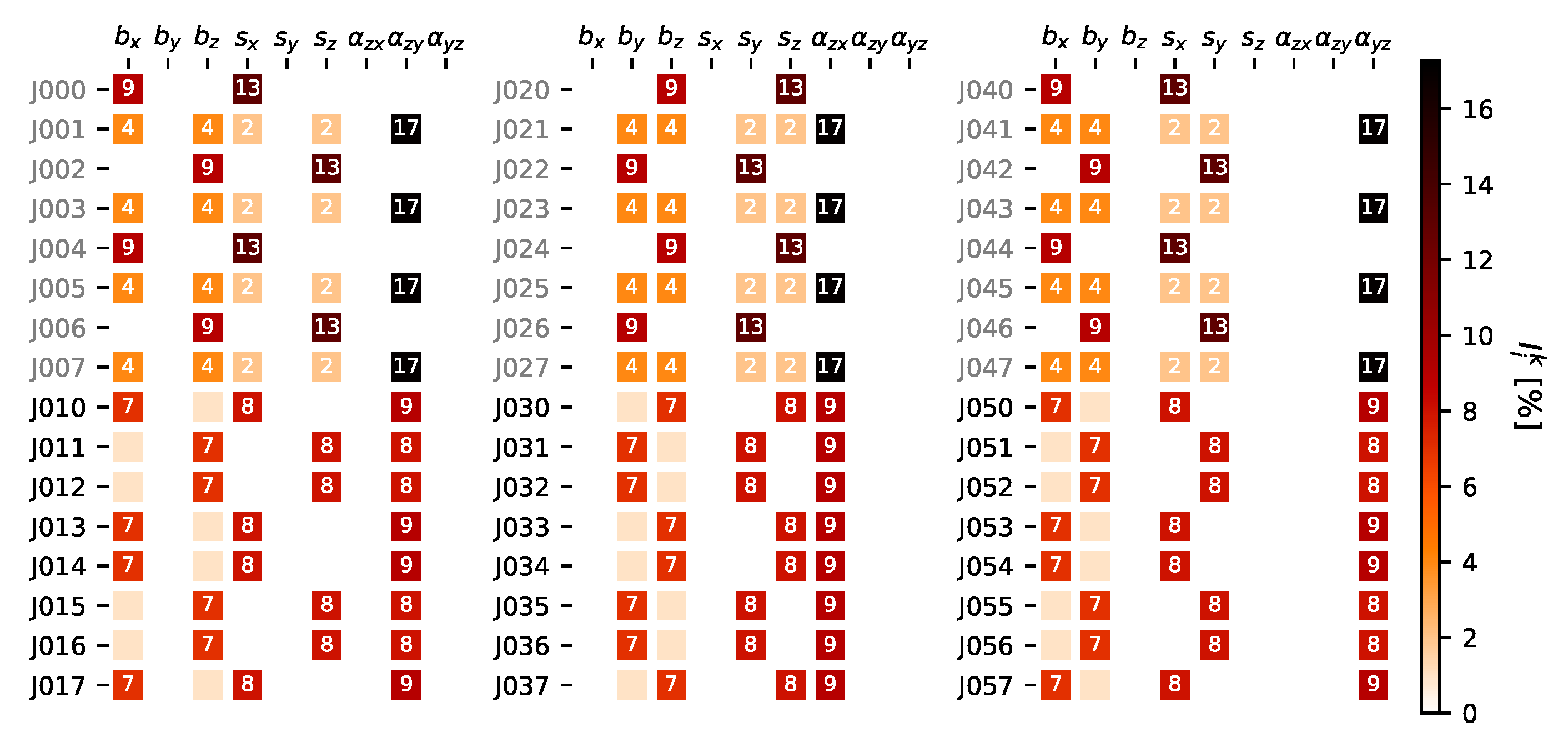
the improvement by means of variance reduction can be computed by:
which is the relative improvement of the
i-th candidate on the
k-th parameter variance. The results for all improvement measures are shown in
Figure 6. Now we can pick the positions with the biggest improvement on the target parameter and might repeat the procedure until a certain exit criterion is met. For a detailed description of this algorithm, please refer to Algorithm A1 in
Appendix B.
The naming of the positions is defined as:
J000 to
J007 are rotations about horizontal
y-axis from 0 gon (
x-axis vertical) to 350 gon in 50 gon steps.
J010 to
J017 are the corresponding 25 gon to 375 gon rotations about horizontal
y-axis. The positions
J020 to
J027 and
J030 to
J037 follow the same scheme about the
x-axis and
J040 to
J047 and
J050 to
J057 about the
z-axis. We can deduce from
Figure 6, that
is best estimated if the rotation axis
j is horizontal and the rotated axis
i (see
Figure 3) forms a ±50 or ±150 gon angle with the gravity vector. These findings match the conclusions from Reference [
38], who did this investigations prior to their estimation process.
For this calibration we picked the eight positions contributing the most on and and stopped, giving a resulting calibration scheme of 32 positions. For comparison the final evaluation investigations have also been done with a full calibration scheme consisting of and giving 48 positions.
4.3. Pole Tilt Compensation
The total effect terms
on the pole components are shown in
Figure 7. IMU specifications and sensor model uncertainties are chosen similar to
Section 4.1, including uncertainties of the mounting parameters from calibration
(
Section 5.2) and a standard deviation
of the yaw
of 0.4 gon. The theoretical standard deviations, again from variance-covariance propagation, are
(horizontal components) and
(height) for
and for example,
(east and height) and
(north) for
. It can be deduced, that again the two important non-orthogonality parameters
together make up almost 40% for near vertical pole tilts (
). With increasing horizontal displacement
the influence of the yaw estimation
increases and has a share of up to almost 75% of the total variance. The effect is similar for both
e and
n components, since we simulated yaw values
from a uniform distribution over the whole spectrum (−200 gon to +200 gon).
It’s important to keep in mind, that VBSA analyzes the stochastic influence of parameters, which does not necessarily agree with deterministic or functional influence. We will revisit this distinction in
Section 5.1.
5. Experiments and Results
To evaluate the proposed methodology a series of experiments were conducted. A consumer-grade MEMS (Micro-Electro-Mechanical Systems) IMU of type
MPU6050 of
InvenSens TDK (see
Figure 8) was used in all the experiments. For the IMU calibration an industrial robot arm
UR5 of
Universal Robots was used as a carrier, see
Figure 8b. For the mounting estimation and evaluation experiment a total station
TS 16 from
Leica Geosystems was used.
First the IMU calibration described in
Section 3.1 was done for the different sensor models
to
(
Section 3) and customized positions schemes
(32 positions) and
(48 positions) based on
(utilizing the same sensor model). During calibration every position was kept static for 5 s.
Secondly the mounting estimation introduced in
Section 3.2 using the different sensor models
giving the corresponding mounting models
. For this a 2.20 m pole was used with 40 evenly distributed positions up to 50 gon tilts. The pole is held static for a period of about 5 to 10 s using a three-legged clamp (see
Figure 8d). The longest possible pole length has been chosen for this calibration, since an error in a mounting parameter has a bigger effect with longer poles.
Finally a pole tilt compensation evaluation experiment was performed, see
Section 5.3.
5.1. IMU Calibration
The results of the different IMU calibrations are shown in
Table 2,
Table 3 and
Table 4. For the first two models
and
the global test of the adjustment (see for example, Reference [
39]) indicates discrepancy in the functional or stochastic model by test values of
and
respectively, see
Table 5. The null hypotheses states that the posterior variance-factor
(computed by weighted sum of squared residuals divided by degree of freedom:
) is equal to the prior variance-factor
. The test quantity
follows a Fisher distribution with parameters
(number of condition equations minus number of parameters) and ∞. The corresponding thresholds can be found in
Table 5. For the 9 parameter models the test value was about
indicating no discrepancy. Since the stochastic model is supposed to be correct for all models, the global test quantity can be treated as indicator for deterministic discrepancies. Again the distinction between deterministic and stochastic influence is important. While the non-orthogonality parameters show the biggest stochastic influence (see sensitivity analysis in
Section 4), the scale parameters show the biggest deterministic influence, indicated by a heavy drop in the test quantity of the global test (
for
against
for
).
The standard deviations of bias and scale drop using 9 parameter models
,
,
, showing that these models might better represent the actual IMU system. Generally the scale factors are quite big, which might be a consequence of the low-cost IMU. The estimated values of models
and
do not differ significantly from each other. Also the standard deviations of bias and scale are quite similar. As expected from the investigations calibration improvement in
Section 4.2, we are able to reduce the standard deviations of the first two non-orthogonality parameters using the extended 32 position scheme
. Nevertheless, the values do not change. A further increase to 48 positions (
) brings no enhancement concerning variance of non-orthogonality parameters. For the relevant non-orthogonality parameters
and
only
is significantly
.
5.2. Mounting Estimation
The results of the mounting estimation Equation (
16) with the corresponding sensor model applied (
is computed by applying
) are shown in
Table 6. From the test quantity of 200 with the bias only model (
), we can see, that there is a clear model discrepancy. The bias and scale model
almost passes the test and for the full models
to
the null hypotheses can be accepted. The first mounting parameter
does not differ significantly between
and all the full models
to
. The non-orthogonality parameter
and
have a similar effect on leveling and tilt compensation and
is insignificant different from 0, hence no difference in the estimated parameter. For the pitch mounting
we can see a difference of approximately
between
and
to
. The accuracy of mounting parameters is also nearly the same for all full model calibrations. A calibration parameter error of 42 mgon (=three times the standard deviation) equals to an error in pole tip coordinates of
for 2.20 m pole length and
for 1.40 pole length.
5.3. Evaluation
Finally the complete pole tilt compensation using the IMU calibration and the mounting estimation is evaluated in an independent experiment. For this a pole length of 1.40 m (mostly used in surveying) is used to measure a known ground point with arbitrary tilts up to 50 gon. Again a three-legged clamp kept the pole static for about 2 to 5 s for each point. The total station is constantly tracking the prism and the measurements are simply time-averaged for each static period. Overall the ground point is measured 75 times.
After applying the mounting
and leveling
of Equation (
9), the yaw (
) can be computed from total station measurements and the known ground point. In fact we use
from ground truth (
, see below) to compute the final tilted pole vector
. This way, we are able to focus on the leveling parameters in our evaluation study. In addition the tilted pole vector can be computed from total station measurements
, see Equation (
14). This
would mean, that the coordinates of the ground point are correctly measured and the pole tilt compensation perfectly yields the tilted pole vector. Therefore we use
as ground truth and analyze the differences
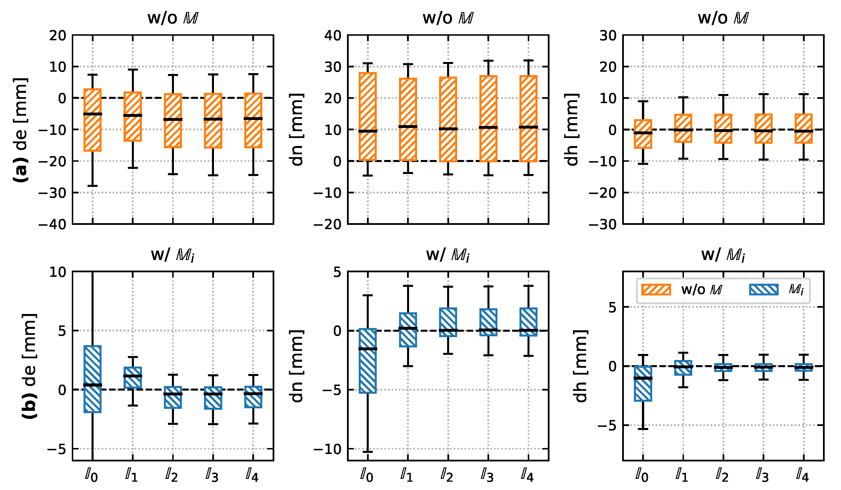
. The results per component are shown in
Figure 9, the numerical results for
Figure 9b are listed in
Table 7. Throughout the experiment, the
x-axis of the IMU was pointing towards the
e-axis of the total station.
Noting the different scales between the subplots (a) (without any mounting applied) and (b), it is obvious, that the application of mounting parameters is crucial for all sensor model
. With the according mounting parameters (
Figure 9b) a Bias only sensor model (
) performs the worst in terms of systematic bias in pole vector components and variability. The second model (
) shows a bias in east component, but the scattering already reduces significantly w.r.t.
. The east component is the one, where errors in the second mounting parameter
and the non-orthogonality parameter
occur (see the differences in
Table 4 and
Table 6 between
/
and
/
). They are consecutive rotations about the
y-axis. There is no significant difference between the full models
to
of different IMU calibration position schemes. We suppose this can have two reasons: first the estimated values of the non-orthogonality parameters
are quite similar for these models, despite the fact that aposteriori variances have improved. Secondly the mounting parameters can mask wrong non-orthogonality parameters, see
Table 6.
The overall ground point (= pole tip) accuracy (), that can be achieved using the low-cost IMU with our approach is about 2.4 mm. Compared to a bias only model of accelerometer triad of 8.0 mm this is an accuracy gain of 69%, compared to a six parameter model (3.0 mm) it corresponds to a gain of 20%. The height component is the most accurate one, since it is the least sensitive one to tilt , which is composed of leveling and mounting parameters.
6. Conclusions
The idea of this paper is to analyze different sensor models of accelerometers triads with respect to leveling applications. In particular for pole tilt compensation, which means computational correction of a slanted position of a pole equipped with a prism. A first prototype with a consumer-grade MEMS IMU and a Raspberry Pi on a simple standard pole from engineering geodesy has been developed. The formalism for pole tilt compensation is successfully validated with this prototype. For that the unknown parameter in this formalism must first be estimated with an appropriate calibration routine, elaborated in this contribution.
The core part of this contribution is related to the question of important parameters in this model. We utilize methods of variance based sensitivity analysis to identify main contributors to the final theoretical uncertainty of the target quantities, for example, tilt angles or pole vector components. We have shown, that the non-orthogonality parameters of the z-axis accelerometer and are the most important both in terms of uncertainty contribution as well as deterministic error introduction. Using this derived insights an iterative application oriented calibration design is proposed to improve the estimated calibration parameters. This concept is formulated to be easily portable to any other calibrations tasks to improve in terms of result accuracy, economics and time saving. Overall sensitivity analysis is useful, both to identify important parameters and to examine how these can be improved.
First the proposed two-part calibration routine consisting of an accelerometer triad calibration using an industrial robot and a mounting estimation with the involved total station is executed. The final evaluation experiment proofs the validity of the proposed models and calibration procedures. With an exact known third orientation angle
we are able to achieve a ground point accuracy of 2.4 mm. The experiment also reveals the necessity of a 9 parameter model consisting of three biases
, three scales
and three non-orthogonality
parameters. Finally three different position schemes for IMU calibration are tested, but showed no performance improvement, it is therefore reasonable to assume that the 24 position scheme from Reference [
26] is sufficient.
Future plans are to repeat the experiments with an industrial grade MEMS IMU and compare the findings between IMUs of different noise level. One can also think about reformulating the compensation model using quaternion attitude representation to overcome singularities inherent in Euler angles and allow the pole for a full-dome probing device. Also for real world application future research has to focus on yaw () estimation, since its uncertainty accounts for up to 75% of the pole components uncertainty.


