An Assessment of Surface Water Detection Methods for Water Resource Management in the Nigerien Sahel


Abstract
1. Introduction
2. Materials and Methods
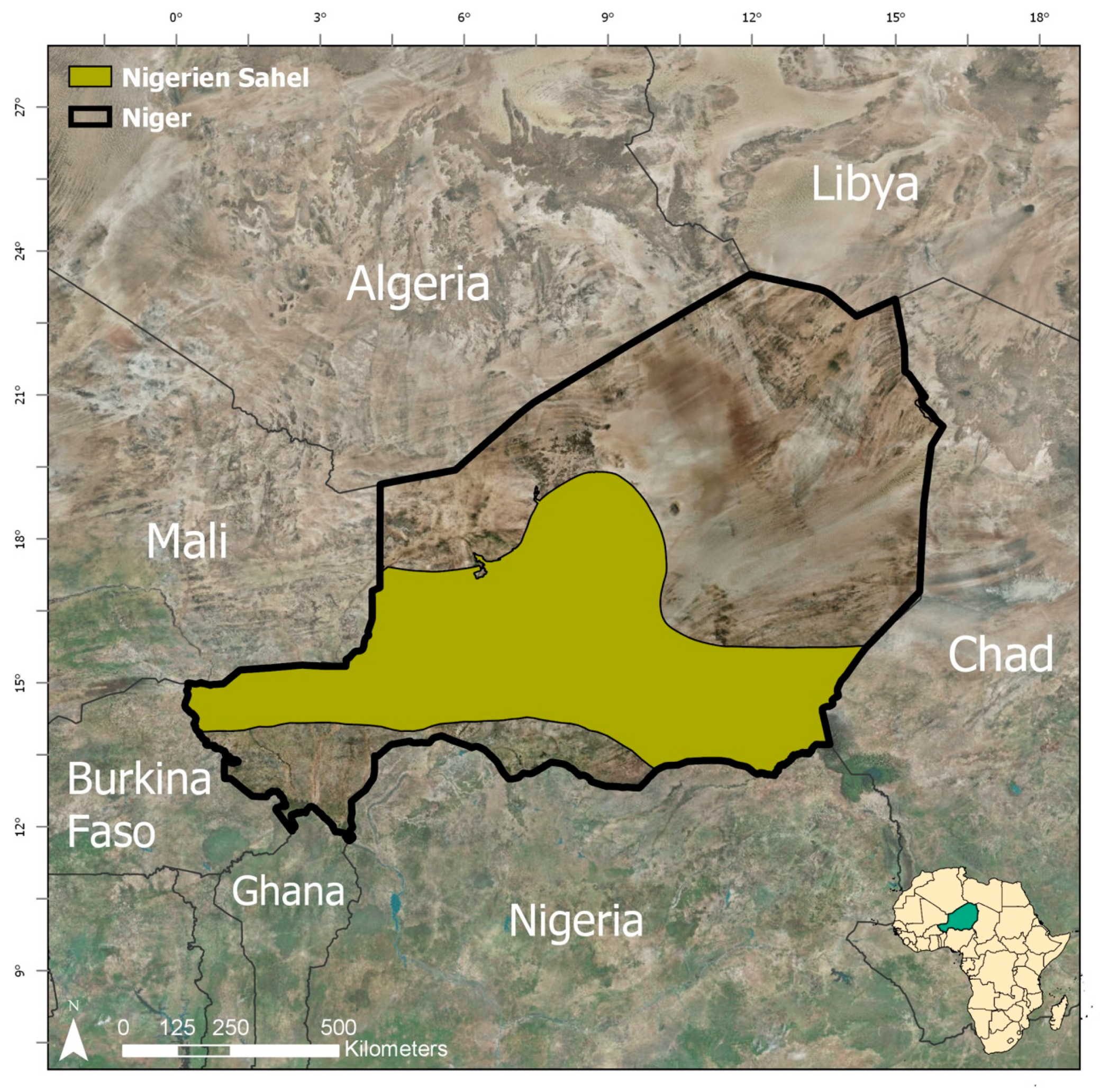
2.1. Study Area
2.2. Data
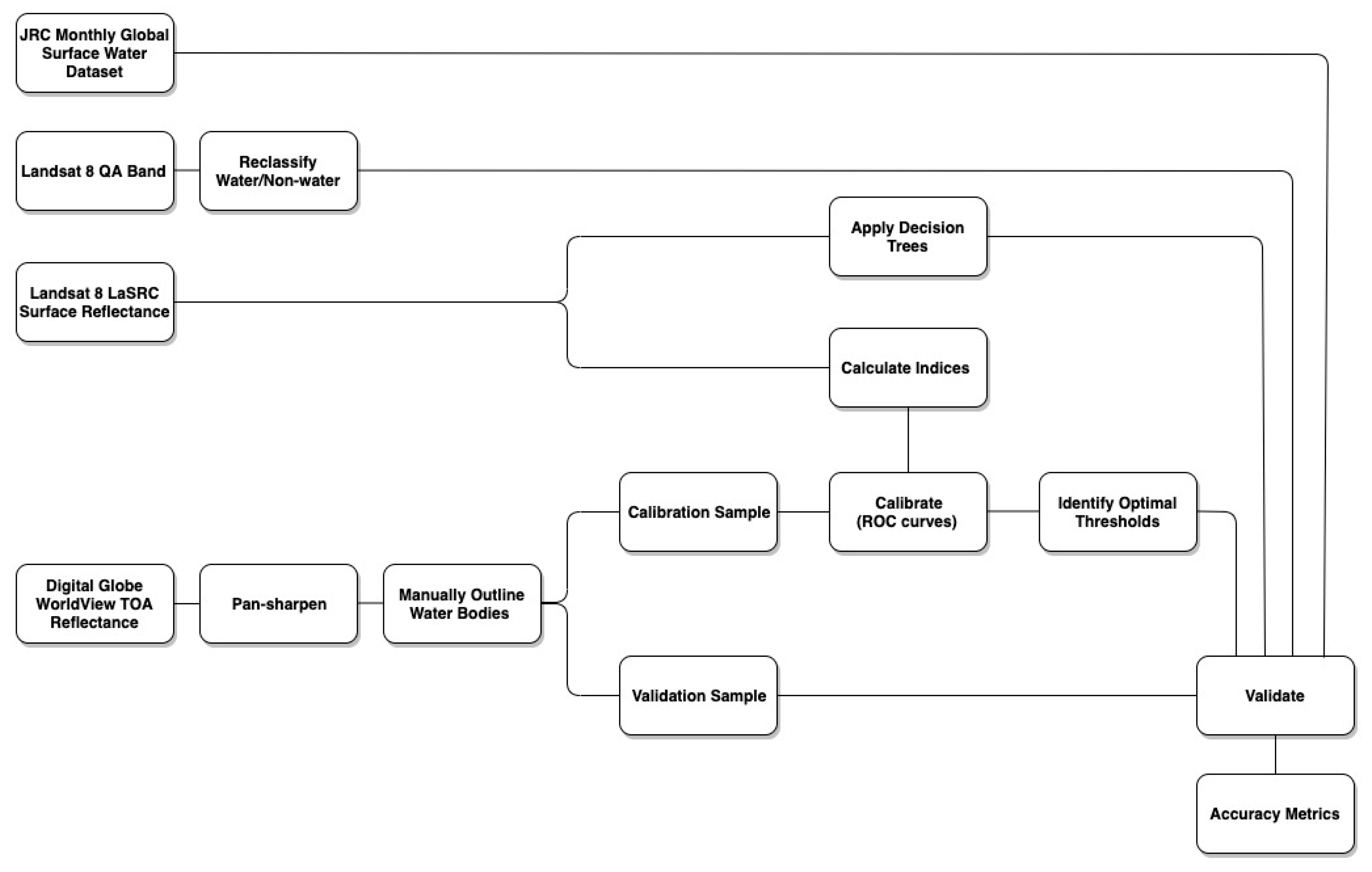
2.3. Methods
3. Results
3.1. Results of Existing Global Surface Water Dataset Assessment
3.2. Results of Spectral Index Assessment
3.3. Results of Decision Tree Assessment
4. Discussion
5. Conclusions
Author Contributions
Funding
Conflicts of Interest
References
- Snorek, J.; Renaud, F.G.; Kloos, J. Divergent adaptation to climate variability: A case study of pastoral and agricultural societies in Niger. Glob. Environ. Chang. 2014, 29, 371–386. [Google Scholar] [CrossRef]
- Snorek, J.; Moser, L.; Renaud, F.G. The production of contested landscapes: Enclosing the pastoral commons in Niger. J. Rural Stud. 2017, 51, 125–140. [Google Scholar] [CrossRef][Green Version]
- Verdin, J.P. Remote sensing of ephemeral water bodies in western Niger. Int. J. Remote Sens. 1996, 17, 733–748. [Google Scholar] [CrossRef]
- Snorek, J.; Terasawa, K.; Stark, J. Climate Change and Conflict in the Sahel: A Policy Brief on Findings from Niger and Burkina Faso; USAID African and Latin American Resilience to Climate Change Project: Burlington, VT, USA, 2014. [Google Scholar]
- McFeeters, S.K. The use of normalized difference water index (NDWI) in the delineation of open water features. Int. J. Remote Sens. 1996, 17, 1425–1432. [Google Scholar] [CrossRef]
- Gao, B. NDWI—A normalized difference water index for remote sensing of vegetation liquid water from space. Remote Sens. Environ. 1996, 58, 257–266. [Google Scholar] [CrossRef]
- Xu, H. Modification of normalized difference water index (NDWI) to enhance open water features in remotely sensed imagery. Int. J. Remote Sens. 2006, 27, 3025–3033. [Google Scholar] [CrossRef]
- Shen, L.; Li, C. Water body extraction from Landsat ETM+ imagery using Adaboost algorithm. In Proceedings of the 18th International Conference on Geoinformatics, Beijing, China, 18–20 June 2010; pp. 1–4. [Google Scholar]
- Baig, M.H.A.; Zhang, L.; Shuai, T.; Tong, Q. Derivation of a tasseled cap transformation based on Landsat 8 at-satellite reflectance. Remote Sens. Lett. 2014, 5, 423–431. [Google Scholar] [CrossRef]
- Feyisa, G.L.; Meilby, H.; Fensholt, R.; Proud, S.R. Automated water extraction index: A new technique for surface water mapping using Landsat imagery. Remote Sens. Environ. 2014, 140, 23–35. [Google Scholar] [CrossRef]
- Tucker, C.J. Red and photographic infrared linear combinations for monitoring vegetation. Remote Sens. Environ. 1979, 2, 127–150. [Google Scholar]
- Fisher, A.; Flood, N.; Danaher, T. Comparing Landsat water index methods for automated water classification in eastern Australia. Remote Sens. Environ. 2016, 175, 167–182. [Google Scholar] [CrossRef]
- Lacaux, J.P.; Tourre, Y.M.; Vignolles, C.; Ndione, J.A.; Lafaye, M. Classification of ponds from high-spatial resolution remote sensing: Application to Rift Valley Fever in Senegal. Remote Sens. Environ. 2007, 106, 66–74. [Google Scholar] [CrossRef]
- Kaptue, A.T.; Hanan, N.P.; Prihodko, L. Characterization of the spatial and temporal variability of surface water in the Soudan-Sahel region of Africa. J. Geophys. Res. Biogeosci. 2013, 118, 1472–1483. [Google Scholar] [CrossRef]
- Gond, V.; Bartholeme, E.; Ouattara, F.; Nonguierma, A.; Bado, L. Surveillance et cartographie des plans d’eau et des zones humides et inondables en regions arides avel l’instrument VEGETATION embarque sur SPOT-4. Int. J. Remote Sens. 2004, 25, 987–1004. [Google Scholar] [CrossRef]
- Halabisky, M.; Moskal, L.M.; Gillespie, A.; Hannam, M. Reconstructing semi-arid wetland surface water dynamics through spectral mixture analysis of a time series of Landsat satellite images (1984–2011). Remote Sens. Environ. 2016, 177, 171–183. [Google Scholar] [CrossRef]
- Huang, C.; Chen, Y.; Zhang, S.; Li, L.; Shi, K.; Liu, R. Spatial downscaling of Suomi NPP-VIIRS image for lake mapping. Water 2017, 9, 834. [Google Scholar] [CrossRef]
- Liu, X.; Deng, R.; Xu, J.; Zhang, F. Coupling the Modified Linear Spectral Mixture Analysis and Pixel-Swapping Methods for Improving Subpixel Water Mapping: Application to the Pearl River Delta, China. Water 2017, 9, 658. [Google Scholar] [CrossRef]
- Acharya, T.D.; Subedi, A.; Lee, D.H. Evaluation of Machine Learning Algorithms for Surface Water Extraction in a Landsat 8 Scene of Nepal. Sensors 2019, 19, 2769. [Google Scholar] [CrossRef]
- Isikdogan, F.; Bovik, A.C.; Passalacqua, P. Surface water mapping by deep learning. IEEE J. Sel. Top. Appl. Earth Obs. Remote Sens. 2017, 10, 4909–4918. [Google Scholar] [CrossRef]
- Malahlela, O.E. Inland waterbody mapping: Towards improving discrimination and extraction of inland surface water features. Int. J. Remote Sens. 2015, 37, 4574–4589. [Google Scholar] [CrossRef]
- Zhou, Y.; Dong, J.; Xiao, X.; Xiao, T.; Yang, Z.; Zhao, G.; Zou, Z.; Qin, Y. Open surface water mapping algorithms: A comparison of water-related spectral indices and sensors. Water 2017, 9, 256. [Google Scholar] [CrossRef]
- Campos, J.C.; Sillero, N.; Brito, J.C. Normalized difference water indexes have dissimilar performances in detecting seasonal and permanent water in the Sahara-Sahel transition zone. J. Hydrol. 2012, 464, 438–446. [Google Scholar] [CrossRef]
- Ji, L.; Zhang, L.; Wylie, B.K. Analysis of dynamic thresholds for the normalized difference water index. Photogramm. Eng. Remote Sens. 2009, 75, 1307–1317. [Google Scholar] [CrossRef]
- Li, W.; Du, Z.; Ling, F.; Zhou, D.; Wang, H.; Gui, Y.; Sun, B.; Zhang, X. A comparison of land surface water mapping using the normalized difference water index from TM, ETM+, and ALI. Remote Sens. 2013, 5, 5530–5549. [Google Scholar] [CrossRef]
- Pekel, J.; Cottam, A.; Gorelick, N.; Belward, A.S. High-resolution mapping of global surface water and its long-term changes. Nature 2016, 540, 418–422. [Google Scholar] [CrossRef]
- USGS. Product Guide: Landsat Surface Reflectance Code (LaSRC) Product v. 4.3; USGS: Sioux Falls, SD, USA, 2018.
- Nicholson, S.E. The West African Sahel: A review of recent studies on the rainfall regime and its interannual variability. ISRN Meteorol. 2013, 2013, 453521. [Google Scholar] [CrossRef]
- Gorelick, N.; Hancher, M.; Dixon, M.; Ilyushchenko, S.; Thau, D.; Moore, R. Google Earth Engine: Planetary-scale geospatial analysis for everyone. Remote Sens. Environ. 2017, 202, 18–27. [Google Scholar] [CrossRef]
- Vermote, E.F.; Tanré, D.; Deuzé, J.L.; Herman, M.; Morcrette, J.J. Second Simulation of the Satellite Signal in the Solar Spectrum, 6S: An overview. IEEE Trans. Geosci. Remote Sens. 1997, 35, 675–686. [Google Scholar] [CrossRef]
- Vermote, E.F.; Saleous, N.; Justice, C.O. Atmospheric correction of MODIS data in the visible to middle infrared: First results. Remote Sens. Environ. 2002, 83, 97–111. [Google Scholar] [CrossRef]
- Herndon, K.E. Applications of Remote Sensing for the Monitoring of Surface Water Dynamics in the Sahel. Master’s Thesis, The University of Alabama in Huntsville, Huntsville, AL, USA, 2018. [Google Scholar]
- Soti, V.; Tran, A.; Bailly, J.S.; Puech, C.; Seen, D.L.; Begue, A. Assessing optical Earth observation systems for mapping and monitoring temporary ponds in arid areas. Int. J. Appl. Earth Obs. Geoinf. 2009, 11, 344–351. [Google Scholar] [CrossRef]
- Donchyts, G.; Schellekens, J.; Winsemius, H.; Eisemann, E.; van de Giesen, N. A 30 m resolution surface water mask including estimation of positional and thematic differences using Landsat 8 SRTM and OpenStreetMap: A case study in the Murray-Darling Basin, Australia. Remote Sens. 2016, 8, 386. [Google Scholar] [CrossRef]
- Metz, C.E. Basic principles of ROC analysis. Seminars Nucl. Med. 1978, 8, 283–298. [Google Scholar] [CrossRef]
- Vermont, J.; Bosson, J.L.; Francois, P.; Robert, C.; Rueff, A.; Demongeot, J. Strategies for graphical threshold determination. Comput. Methods Programs Biomed. 1991, 35, 141–150. [Google Scholar] [CrossRef]


| Satellite/Sensor | Data Source | Image Resolution | Image ID | Date |
|---|---|---|---|---|
| Landsat 8 OLI | USGS ESPA | 30 m | LC81910492015294LGN01 | 21 October 2015 |
| LC81910502017364LGN01 | 29 December 2017 | |||
| LC81910492017268LGN01 | 24 September 2017 | |||
| LC81910492016121LGN01 | 30 April 2016 | |||
| WorldView-3 | Digital Globe | 2 m (pansharpened to 0.5 m) | 1040010012220E00 | 21 October 2015 |
| 10400100356E6500 | 29 December 2017 | |||
| WorldView-2 | Digital Globe | 2 m (pansharpened to 0.5 m) | 1030010070CF0800 | 24 September 2017 |
| 10300100547AA300 | 30 April 2016 |
| DG Scene | Scene Area (km2) | Water Surface Area (km2) | Water Perimeter (km) | Rasterized Surface Area (km2) |
|---|---|---|---|---|
| 1040010012220E00 | 1463.17 | 2.08 | 115.4 | 1.95 |
| 10400100356E6500 | 1576.51 | 2.26 | 58.92 | 2.23 |
| 1030010070CF0800 | 1923.60 | 8.78 | 181.26 | 8.54 |
| 10300100547AA300 | 1988.15 | 4.77 | 19.23 | 4.77 |
| Name | Citation | Equation | Bands Used | |||||
|---|---|---|---|---|---|---|---|---|
| B | G | R | NIR | SWIR1 | SWIR2 | |||
| Near Infrared | - | NIR | - | - | - | X | - | - |
| SWIR 1 | - | SWIR 1 | - | - | - | - | X | - |
| SWIR 2 | - | SWIR 2 | - | - | - | - | - | X |
| NIR-Red Ratio | 13 | NIR/RED | - | - | X | X | - | - |
| Red-Green Ratio | 13 | RED/GREEN | - | X | X | - | - | - |
| Normalized Difference Water Index (NDWI) | 5 | NDWI = (GREEN − NIR)/(GREEN + NIR) | - | X | - | X | - | - |
| Normalized Difference Moisture Index (NDMI) | 6 | NDMI = (NIR − SWIR)/(NIR + SWIR) | - | - | - | X | X | - |
| Modified Normalized Difference Water Index (MNDWI) | 7 | MNDWI = (GREEN − SWIR)/(GREEN + SWIR) | - | X | - | - | X | - |
| Normalized Difference Pond Index (NDPI) | 13 | NDPI = (SWIR − GREEN)/(SWIR + GREEN) | - | X | - | - | X | - |
| Water Ratio Index (WRI) | 8 | WRI = (GREEN + RED)/(NIR+ SWIR) | - | X | X | X | X | - |
| Tasseled Cap Wetness (TCW) | 9 | TCW = 0.1511 × BLUE + 0.1973 × GREEN + 0.3283 × RED +0.3407 × NIR − 0.7117 × SWIR1 − 0.4559 × SWIR2 | X | X | X | X | X | X |
| Automated Water Extraction Index (AWEIsh) | 10 | AWEI(sh) = BLUE + 2.5 × GREEN − 1.5 × (NIR+SWIR1) − 0.25 × SWIR2 | X | X | - | X | X | X |
| Automated Water Extraction Index (AWEInsh) | 10 | AWEI(nsh) = 4 × (GREEN − SWIR1) − (0.25 × NIR + 2.75 × SWIR1) | - | X | - | X | X | - |
| Normalized Difference Vegetation Index (NDVI) | 11 | NDVI = (NIR − RED)/(NIR + RED | - | - | X | X | - | - |
| WI2015 | 12 | 1.7204 + 171(GREEN) + 3(RED) + 70(NIR) + 45(SWIR1) + 71(SWIR2) | - | X | X | X | X | X |
| MNDWI and NDVI | 14 | Water where NDVI < 0 and MNDWI > 0 | - | X | X | X | X | - |
| Simple Water Index (SWI) | 21 | SWI = 1/, values <5 are classified as water | X | - | - | - | X | - |
| NDWI, NDVI, SWIR1 | 15 |
| - | X | X | X | X | - |
| Dataset | Date | OA | FP | FN |
|---|---|---|---|---|
| Landsat 8 QA band | 21 October 2015 | 0.82 | <1% | 0.18 |
| 29 December 2017 | 0.78 | 0 | 0.22 | |
| 24 September 2017 | 0.93 | 0 | 0.07 | |
| 30 April 2016 | 0.77 | 0 | 0.20 | |
| JRC GSW | October 2015 | 0.84 | <1% | 0.15 |
| Algorithm | Scene 1 (Calibrated to Scene 1) | Scene 2 (Calibrated to Scene 2) | Scene 3 (Calibrated to Scene 3) | Scene 4 (Calibrated to Scene 4) | All Scenes (Calibrated to All Scenes) | |||||
|---|---|---|---|---|---|---|---|---|---|---|
| Optimal Threshold | OA | Optimal Threshold | OA | Optimal Threshold | OA | Optimal Threshold | OA | Optimal Threshold | OA | |
| NIR | 0.2965 | 0.70 | 0.4104 | 0.49 | 0.1659 | 0.89 | 0.2193 | 0.79 | 0.2338 | 0.75 |
| SWIR 1 | 0.3032 | 0.96 | 0.3450 | 0.98 | 0.2110 | 0.99 | 0.2750 | 0.99 | 0.2522 | 0.97 |
| SWIR 2 | 0.2035 | 0.95 | 0.2440 | 0.98 | 0.1210 | 0.99 | 0.2090 | 0.99 | 0.1652 | 0.97 |
| NIR/R Ratio | 1.2857 | 0.73 | 1.1587 | 0.96 | 1.1205 | 0.95 | 1.1754 | 0.63 | 1.1859 | 0.82 |
| R/G Ratio | 1.3935 | 0.84 | 1.4621 | 0.83 | 1.2413 | 0.94 | 1.2600 | 0.99 | 1.3774 | 0.84 |
| NDWI | −0.2817 | 0.83 | −0.2548 | 0.96 | −0.2329 | 0.96 | −0.1976 | 0.96 | −0.2498 | 0.88 |
| NDMI | −0.0365 | 0.96 | 0.0158 | 0.98 | 0.0149 | 0.98 | −0.0753 | 0.99 | 0.0149 | 0.98 |
| MNDWI | −0.3378 | 0.97 | −0.2082 | 0.98 | −0.3335 | 0.99 | −0.3300 | 0.99 | −0.3350 | 0.98 |
| NDPI | 0.3378 | 0.97 | 0.2080 | 0.98 | 0.3340 | 0.99 | 0.3300 | 0.99 | 0.3350 | 0.98 |
| WRI | 0.6056 | 0.97 | 0.7320 | 0.98 | 0.5799 | 0.97 | 0.6253 | 0.99 | 0.6250 | 0.97 |
| TCW | −0.1047 | 0.96 | −0.0555 | 0.98 | −0.0803 | 0.99 | −0.1410 | 0.99 | −0.1118 | 0.98 |
| AWEIsh | −0.4187 | 0.96 | −0.4455 | 0.98 | −0.3893 | 0.98 | −0.4040 | 0.99 | −0.4078 | 0.98 |
| AWEInsh | −1.4701 | 0.96 | −1.4995 | 0.98 | −1.0600 | 0.99 | −1.4200 | 0.99 | −1.3835 | 0.98 |
| SWI | -* | 0.81 | -* | 0.95 | -* | 0.80 | -* | 0.77 | -* | 0.83 |
| NDVI | 0.1250 | 0.73 | 0.0735 | 0.96 | 0.0568 | 0.95 | 0.0806 | 0.63 | 0.0850 | 0.82 |
| WI2015 | 80.0887 | 0.79 | 98.5396 | 0.90 | 52.8095 | 0.94 | 63.4000 | 0.97 | 66.6648 | 0.69 |
| Kaptue | -* | 0.87 | -* | 0.91 | -* | 0.95 | -* | 0.77 | -* | 0.88 |
| Gond | -* | 0.93 | -* | 0.97 | -* | 0.95 | -* | 0.97 | -* | 0.96 |
© 2020 by the authors. Licensee MDPI, Basel, Switzerland. This article is an open access article distributed under the terms and conditions of the Creative Commons Attribution (CC BY) license (http://creativecommons.org/licenses/by/4.0/).
Share and Cite
Herndon, K.; Muench, R.; Cherrington, E.; Griffin, R. An Assessment of Surface Water Detection Methods for Water Resource Management in the Nigerien Sahel. Sensors 2020, 20, 431. https://doi.org/10.3390/s20020431
Herndon K, Muench R, Cherrington E, Griffin R. An Assessment of Surface Water Detection Methods for Water Resource Management in the Nigerien Sahel. Sensors. 2020; 20(2):431. https://doi.org/10.3390/s20020431
Chicago/Turabian StyleHerndon, Kelsey, Rebekke Muench, Emil Cherrington, and Robert Griffin. 2020. "An Assessment of Surface Water Detection Methods for Water Resource Management in the Nigerien Sahel" Sensors 20, no. 2: 431. https://doi.org/10.3390/s20020431
APA StyleHerndon, K., Muench, R., Cherrington, E., & Griffin, R. (2020). An Assessment of Surface Water Detection Methods for Water Resource Management in the Nigerien Sahel. Sensors, 20(2), 431. https://doi.org/10.3390/s20020431