Article

A Personalized Diagnosis Method to Detect Faults in a Bearing Based on Acceleration Sensors and an FEM Simulation Driving Support Vector Machine

1
College of Mechanical and Electrical Engineering, Wenzhou University, Wenzhou 325035, China
2
Huadian Electric Power Research Institute, Hangzhou 310030, China
*
Author to whom correspondence should be addressed.
Sensors 2020, 20(2), 420; https://doi.org/10.3390/s20020420
Submission received: 6 December 2019 / Revised: 8 January 2020 / Accepted: 9 January 2020 / Published: 11 January 2020

Abstract

:
Classification of faults in mechanical components using machine learning is a hot topic in the field of science and engineering. Generally, every real-world running mechanical system exhibits personalized vibration behaviors that can be measured with acceleration sensors. However, faulty samples of such systems are difficult to obtain. Therefore, machine learning methods, such as support vector machine (SVM), neural network (NNs), etc., fail to obtain agreeable fault detection results through smart sensors. A personalized diagnosis fault method is proposed to activate the smart sensor networks using finite element method (FEM) simulations. The method includes three steps. Firstly, the cosine similarity updated FEM models with faults are constructed to obtain simulation signals (fault samples). Secondly, every simulation signal is separated into sub-signals to solve the time-domain indexes to generate the faulty training samples. Finally, the measured signals of unknown samples (testing samples) are inserted into the trained SVM to classify faults. The personalized diagnosis method is applied to detect bearing faults of a public bearing dataset. The classification accuracy ratios of six types of faults are 90% and 92.5%, 87.5% and 87.5%, 85%, and 82.5%, respectively. It confirms that the present personalized diagnosis method is effectiveness to detect faults in the absence of fault samples.

1. Introduction

With the rapid development of artificial intelligence (AI) technology, machine learning methods have been widely used in fault diagnosis of mechanical components. Rolling bearings, as important components in rotating machinery, they exhibit personalized vibration behaviors under different work conditions. The running state of bearings directly affects the reliability and stability of the entire machine. Thus, in order to detect the faults in bearings, many researchers have proposed different intelligent diagnosis methods based on machine learning methods or artificial intelligence models [1,2,3]. Wang et al. [4] presented convolutional neural network-based hidden Markov models (CNN-HMMs) to classify multi faults in a bearing. To enlarge the application cases of training samples collected from fault simulators, an intelligent fault diagnosis approach was proposed using transfer learning to transfer fault samples from laboratory bearings to locomotive bearings [5]. By using limited fault samples as training and testing samples, the performance of machine learning methods have been verified to detect faults in bearings, such as extreme learning machine (ELM), support vector machine (SVM), neural networks (NNs) [6,7,8,9], etc. However, in the real world, it is difficult to obtain sufficient suitable training samples to represent various kinds of bearing faults that may occur in actual mechanical systems. Therefore, various machine learning methods have been greatly limited in engineering applications for the lack of fault training samples.
To fully understand the fault mechanism and obtain agreeable fault detection results, many researchers performed numerical simulations to analyze faults. To detect faults online in nonlinear continuous systems, Bregon et al. [10] used the simulation and state observer models to obtain the final fault diagnosis results. To detect the abnormal conditions of structures, two kinds of wavelet-based numerical simulation models were carried out to calculate the dynamic responses of a shaft [11,12]. Thereafter, Xiang and Zhong [13] further proposed a novel fault diagnosis scheme using finite element method (FEM), wavelet packet transform (WPT), and SVM. To detect faults in reciprocating machine, Wang et al. [14] proposed a combination method using the minimum entropy deconvolution (MED) and FEM modal analysis determined band-pass filter to detect faults in an axial piston pump. Generally, as a powerful tool, FEM simulation can be employed to obtain a large number of numerical data/signals at a lower experimental cost, especially for those that are difficult to obtain through physical experiments.
FEM models are constructed on the basis of a highly idealized engineering design, and the dynamic responses of FEM simulations and physical experiments are usually quite different. In order to obtain effective FEM simulation results similar to those in real-world running mechanical systems, it is necessary to update the FEM model. As an optimization problem, the FEM model updating is achieved by correcting the design parameters, such as boundary conditions and materials [15]. According to the dynamic theory of mechanical system, the dynamic information in different assembly and working states will be carried in the corresponding vibration signals [16]. Therefore, various FEM model parameters can be corrected effectively by comparing the measured signals with the FEM simulation signals using similarity indexes, such as the cosine similarity, Theil’s inequality coefficient, etc. [17].
As one of the key problems in the intelligent diagnosis, the selection of feature vectors is affect diagnosis result directly. Generally, feature vectors are generated by calculating the feature indexes in time, frequency and time-frequency domains. Chen et al. [18] proposed an approach including six indexes (e.g., mean value, root mean square, standard deviation, skewness, kurtosis and shape indicator) and two indexes (e.g., mean frequency and standard deviation frequency) in the time frequency domains, respectively to construct a feature set to train the SVM. Liu et al. [19] used a hybrid time frequency analysis method to get the feature information to classify gear faults.
SVM is a pattern recognition approach widely used in fault classification [20]. Based on Vapnik Chervonenkis (VC) dimension theory and structural risk minimization (SRM) principle, SVM can be used to solve the nonlinear and high dimensional problems. However, due to the lack of fault training samples, SVM has not been successfully applied to real-world running mechanical systems.
Recently, motivated by personalized medicine, Xiang [13] developed a personalized diagnosis concept for mechanical fault diagnosis by the combination of numerical simulations and machine learning methods or artificial intelligence models. If the FEM model can effectively represent the real-world running mechanical systems, the lack of fault training samples will be inexpensively obtained by FEM simulations. Thereafter, machine learning methods or artificial intelligence models will be activated for the diagnosis of mechanical faults under different working conditions. In this paper, we proposed a new personalized diagnosis method called FEM simulation driving SVM to detect faults in a bearing. In Section 2, the basic principle of the personalized diagnosis method is introduced. In Section 3, an example is given to show the performance of the present method to classify six types of faults in experimental test rigs. Concluding remarks of this study are given in Section 4.

2. The Basic Principle of Personalized Diagnosis Method

2.1. Cosine Similarity-Based FEM Model Updating Technique

As we know, vibration of mechanical system is the external reflection of its intrinsic dynamic characteristics, thus vibration signals (dynamic responses) can be used to determine the corresponding main parameters of FEM model, such as materials and boundary conditions. Many researchers have done researches on model parameter identification and fault diagnosis based on vibration signals [21,22,23]. Sarin et al. [24] made comparative study residual errors between time-domain signals of simulations and experiments, and further provided a theoretical basis for model updating. Zapico-Valle et al. [25] defined a residual value between FEM simulation and experimental signals to search the minimum residual value using optimization methods for the purpose of FEM model updating. Here, we directly use the cosine similarity between the time-domain vibration signals of FEM simulation and experimental measurement to update the FEM model of a bearing by adjusting the corresponding parameters. The cosine similarity between the measured and the FEM simulation signals is defined by:
c o s ( θ ) = i = 1 n ( x i × y i ) / ( i = 1 n ( x i ) 2 × i = 1 n ( y i ) 2 ) = X Y X × Y ,
where X and Y represent the measured and simulation signals, respectively. When the closer the value of cos(θ) is to 1, the more similar the two signals are. Generally, in engineering applications, cos(θ) > 0.6 will lead to a satisfactory result [26].

2.2. A Brief Review of SVM

Consider a training set S:
S = { x i , y i } i = 1 l ,
where xi Є Rl, yi Є {-1,+1}, and l is the number of samples.
The aim of SVM is to determine an optimal hyper plane for separating one from the others by using the training dataset. To get the ideal hyper plane, the dual optimization problem is often mentioned in SVM as:
m i n 1 2 i = 1 l j = 1 l α i α j y i y j K ( x i , y j ) + i = 1 l α i , s . t . i = 1 l y i α i 0 α i C , i = 1 , 2 , , l ,
where αi is the Lagrange multiplier coefficient obtained by dealing with the dual optimization in the process of the SVM training; K(xi, yi) is referred to as the kernel function; C > 0 is the error penalty parameter.
There are many forms of the kernel function. The radial basis function (RBF) kernel is employed in this paper for the highest accuracy ratio of classification. How to choose the tradeoff parameters ρ1 (the width of RBF) and C is a difficult task in the application of SVM. A possible way is suggested by Xiang et al. [27] suggested that the simulation investigation should proceed first to obtain the relative best parameters ρ1 and C, and hence, ρ1 = 1.05 and C = 10 were employed in the present investigation.

2.3. The Personalized Diagnosis Method by Using FEM Simulation and SVM

For the bearings under different running sates, the vibration response signals exhibit personalized characteristics. In the fault diagnosis of bearings, a generalized fault samples definitely not available for all the bearings. Therefore, a new idea for personalized fault diagnosis is developed using FEM simulation to activate SVM. Figure 1 shows the flowchart of the present method.

2.3.1. Construct and Update the FEM Model for a Mechanical System

FEM model of a mechanical systems is constructed using the commercial FEM software ANSYS. To keep the FEM model effectively represent the corresponding physical mechanical system, the cosine similarity-based FEM model updating technique is used to determine the model parameters based on the comparison of the time-domain signals obtained by FEM simulations and measurements. If the value of cosine similarity is larger than 0.6, the FEM model can well represent its physical one. Moreover, the faulty models will be inserted into the FEM model to simulate the dynamic response of mechanical system with faults.

2.3.2. Obtain the Faulty Training Samples

The FEM models of the mechanical systems with different faults are calculated to obtain the simulation vibration signals in time-domain. Then, each simulation signal is divided into sub-signals with the same length in time domain, and the sixteen time-domain indexes (as shown in Table 1) of each sub-signal are further calculated. Therefore, the number of training samples corresponding to each fault is the same, which ensures the balance of the samples.

2.3.3. Fault Classification Using SVM

The fault training samples formed by the time-domain indexes are used as inputs to train SVM. Same as the processing of simulation signals, each measured signal (the fault type is unknown) is employed to generate the testing samples to the trained SVM, and fault patterns are finally identified.

3. Experimental Investigations

In this section, experimental investigations of a public bearing dataset were carried out, which proves that the personalized diagnosis method is feasible in bearing faults diagnosis using FEM simulation driving SVM. In order to ensure the reliability of the measured signals, the bearing data are from the Bearing Data Centre at Case Western Reserve University (CWRU), as referred to in the website [28]. The drive-end bearing is taken as the experimental object, and the sampling frequency is 6 kHz.

3.1. Construction and Updating of Bearing FEM Model

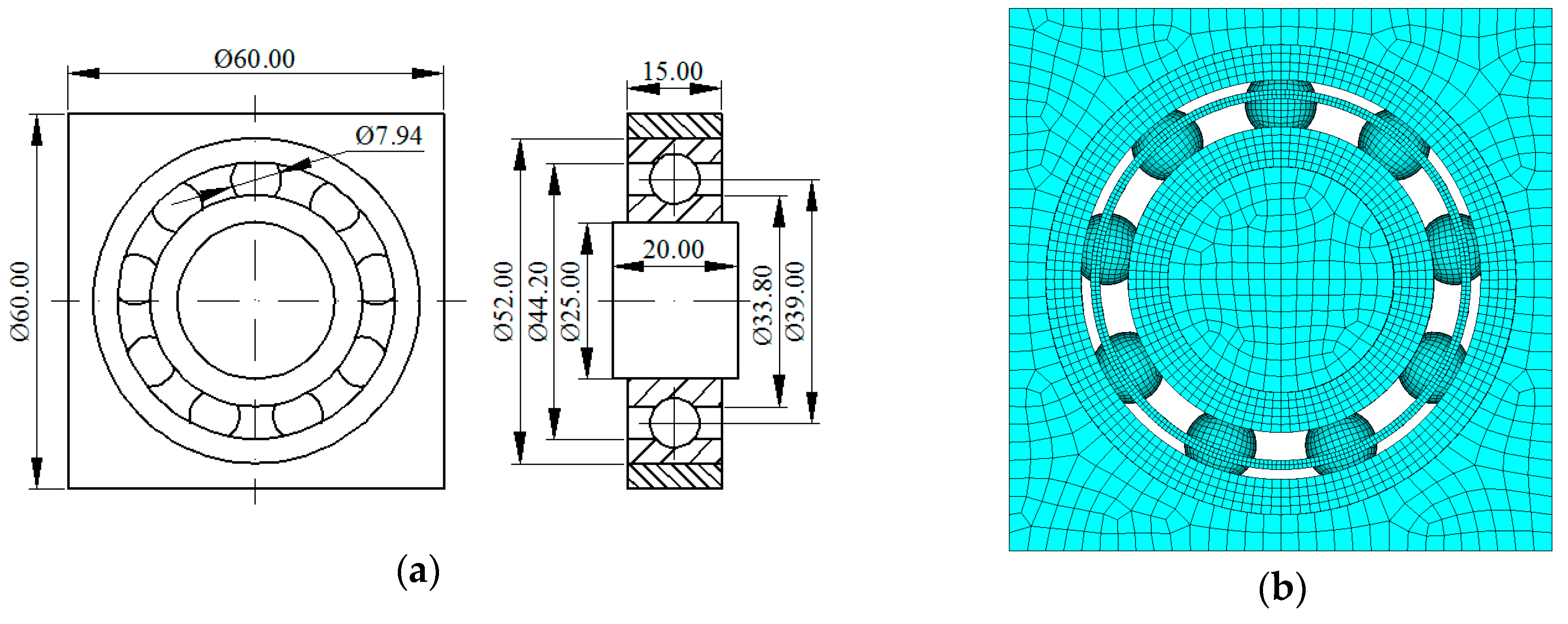
According to the experiment of CWRU, the geometrical dimensions of bearing were determined, shown in Figure 2a. Using commercial finite element analysis (FEA) software ANSYS to construct a three-dimensional (3D) FEM model of the bearing with the bearing seat and shaft, as shown in Figure 2b.
In constructing the FEM model of the bearing, 3D solid element (SOLID164) and shell element (SHELL163) are employed to mesh the body and inner surface of inner ring (for applying the rotating loading), respectively. In order to reduce the computing time and improve the calculation accuracy, the element size is changed according to the components of bearing, as shown in Table 2. Figure 2b shows the result of meshing, and the total FEM model contains 71,976 elements with 73,133 nodes. All the components of bearing are constructed with line elastic material: density ρ = 7860 kg/m3, elastic modulus E = 2.06 × 10 Pa, and Poisson’s ratio μ = 0.3.
Consider the actual working condition, three contact pairs are defined in the FEM model:
(1) S1, a contact pair between the balls and inner ring.
(2) S2, a contact pair between the balls and outer ring.
(3) S3, a contact pair between the outer ring and bearing seat.
Due to the max radial load of bearing is known to be Fr = 14 kN, the dynamic friction coefficients f1 and f2 of S1 and S2, respectively, can be determined using the geometry and material parameters [29,30,31] to f1 = 0.02 and f2 = 0.016, respectively. Generally, the contact damping c of the bearing in running state is variable, while the damping coefficient λ is near constant [32,33,34] and is suggested to λ = 0.02 [35]. To set the contact stiffness, a normal contact stiffness factor FKN is employed in ANSYS to estimate the contact stiffness based on the material properties and the elemental deformations. FKN is suggested to be the maximum value within the interval [0.1, 1] to avoid penetration and keep the contact stress unchanged using static analysis [36]. Based on the static analysis of bearing under Fr =14 kN, the FKN=0.12 can be empirically determined with f1 = 0.02, f2 = 0.016, and λ = 0.02 . The contact parameters of the FEM model are finally listed in Table 3.
In the FEM simulations, the shaft and inner ring are combined as one volume. The displacement constraining of the model are: the axial degree-of-freedom (DOF) of bearing, the rotating DOF of outer ring, and all the DOFs on the outer surface of bearing seat.
However, the loads of bearing are unknown, include the gravity load of shaft Fg, the eccentric load caused by machining error Fe, and the preload of inner ring Fro, which are the main factors affecting the vibration response of the bearing. Therefore, the three loads are the sensitive parameters to be updated using the cosine similarity cos(θ). Referring to the rotating load of bearing in the actual experiment, the rotating speed n = 1797 rpm is applied to the inner surface of the inner ring. Fg is preliminary set in the range from 100 N to 1000 N. Meanwhile, Fe is applied to the upper surface of inner ring. According to the general coaxiality requirement of a shaft, the maximum eccentric distance of the shaft is limited to 0.01 mm. Then Fe is accordingly updated in the range of 0 to 0.2 MPa. Moreover, Fi is applied on the inner surface of the inner ring to make each ball fully contact with the raceway. According to Reference [37], the radial preload of inner ring Fao can be calculated:
F ao = 1.13 × 10 12 D w 3 d m ( 1 γ 2 ) ( 1 γ ) × Z n 2 sin β sin α / f 1 + 1.9 F r t g α ,
F ro = F ao cos α / S i ,
where Dw denote the diameter of ball; dm is the inner diameter of bearing; Z is the number of balls; α = 0.19 rad is the contact angular of the bearing; β is the self-rotation angle of ball, β=α; γ denotes the structural parameter of bearing, γ = 2 D w cos α / ( D + d ) ; D and d are the outer and inner diameters of bearing (mm), respectively; and Si is the area of inner surface of inner ring. Using Equation (5), Fro can be determined.
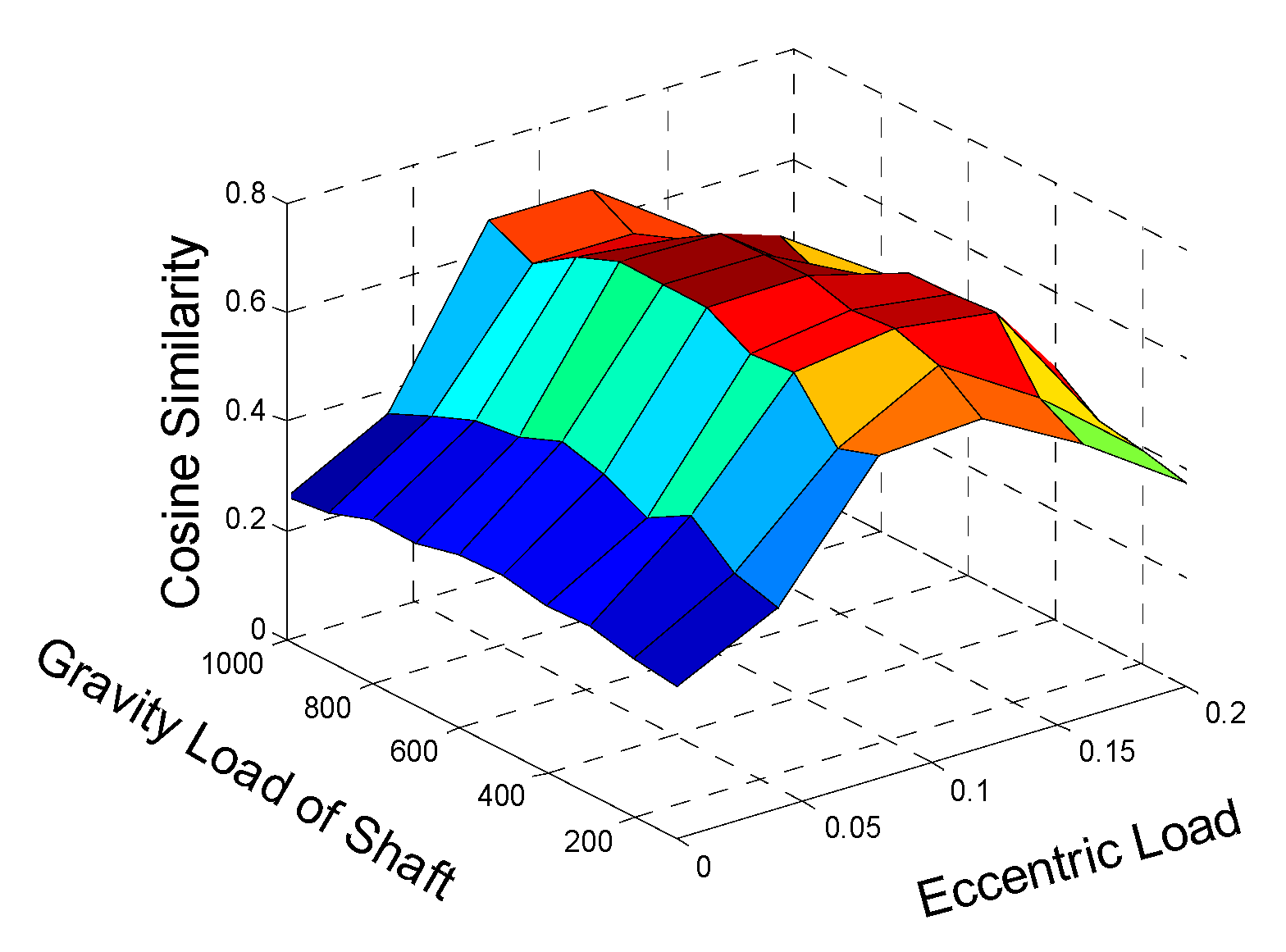
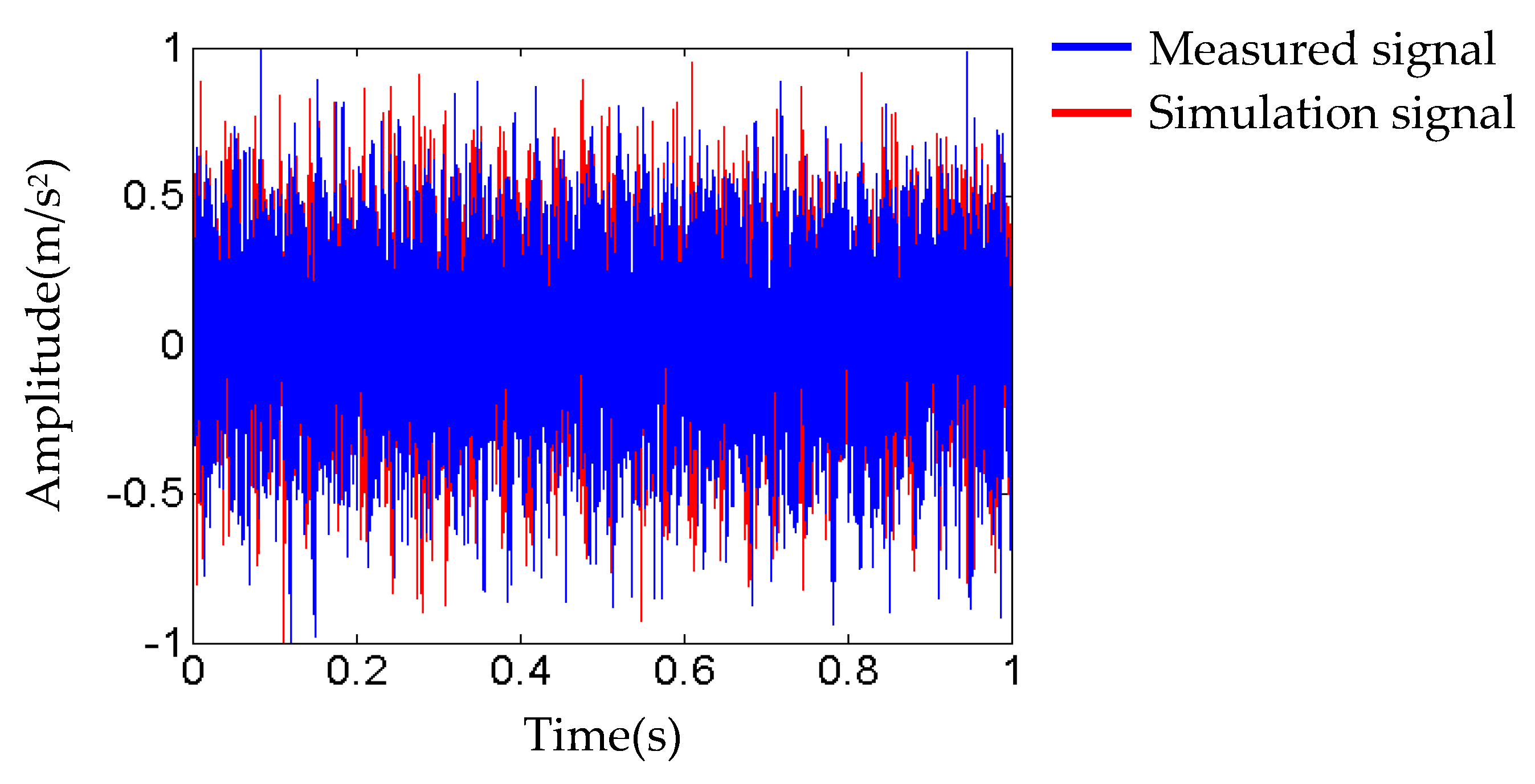
Through iteratively adjusting the selected load parameters (Fg, Fe, and Fro) according to the flowchart shown in Figure 1, we finally obtain the maximum cosine similarity cos(θ) = 0.618. The changing trend of cosine similarity values are shown in Table 4 and Figure 3. Figure 4 shows the comparison between measured and simulated signals when cos(θ) = 0.618. The two signals are matched well at a certain degree, which proves that the updated FEM model constructed using the relative optimal parameters (shown in Table 3) is agreeable.

3.2. Generation of Simulation Fault Training Samples

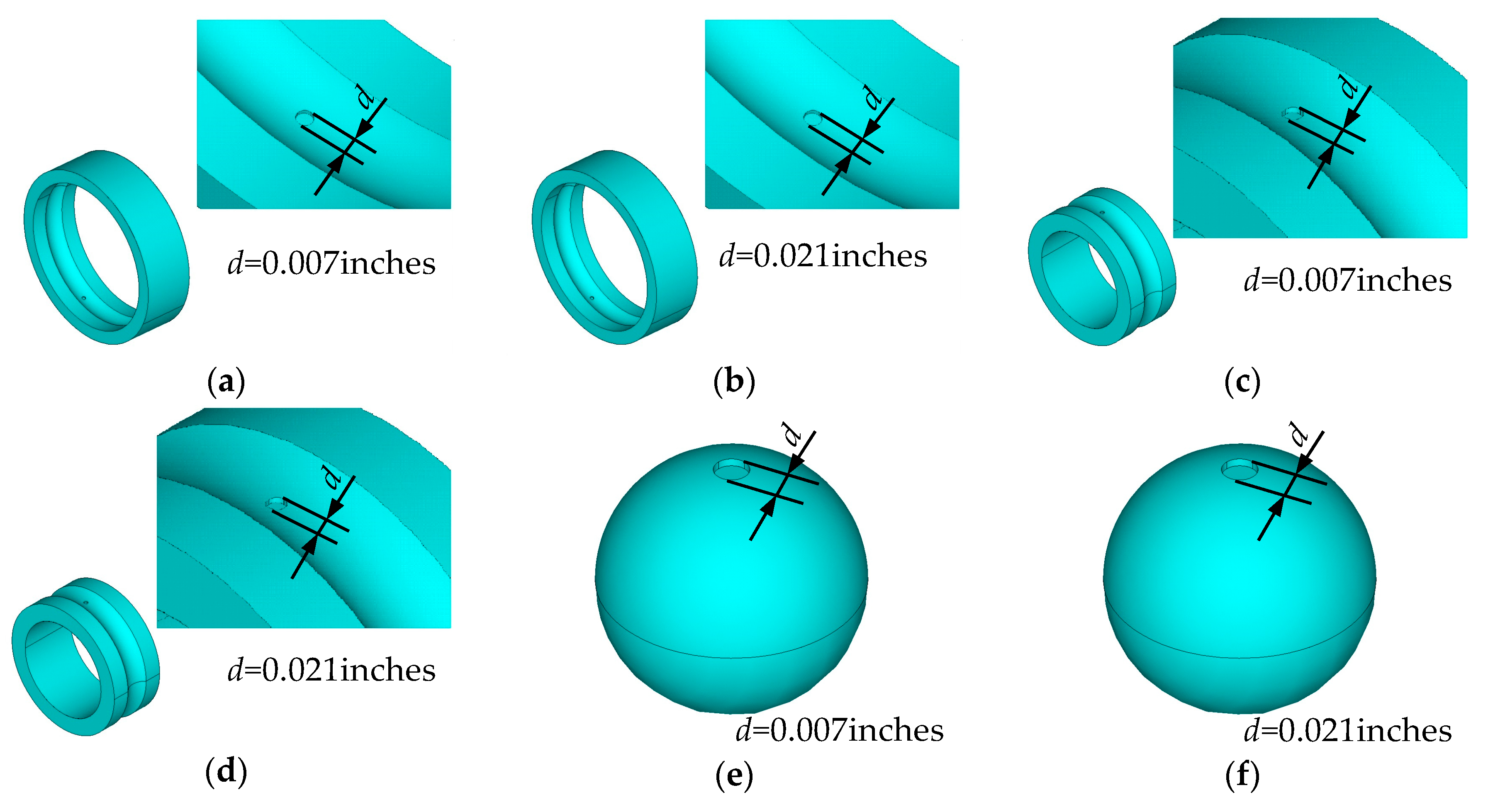
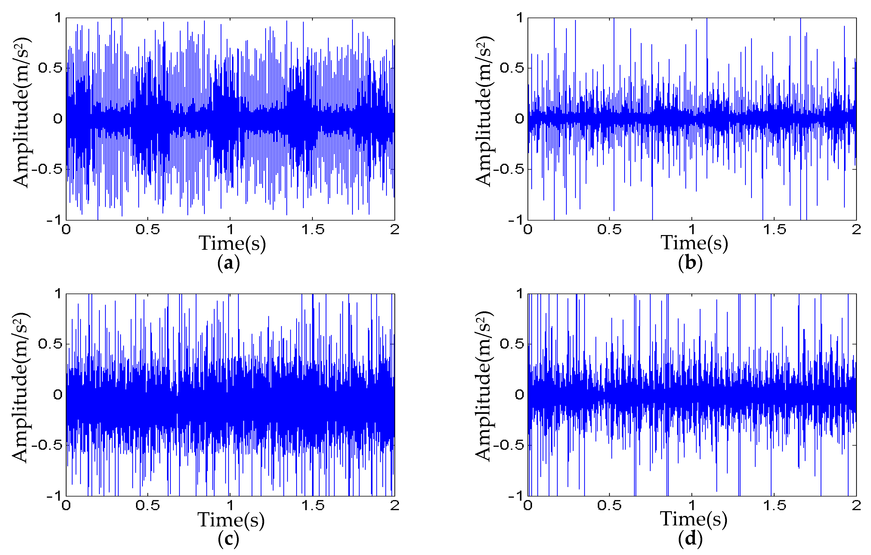
According to bearing data from CWRU, six types of bearing faults (denoted by T1, T2, T3, T4, T5, and T6) are considered, as shown in Figure 5. Using the updated FEM model parameters (shown in Table 4), the FEM models with the above six types of faults are constructed to generate the simulation signals, and the length of each simulation signal is 12,000 data points, as shown in Figure 6.
For getting satisfactory performance in fault classification, each simulation signal is normalized and divided into 40 sub-signals in time-domain (12,000 data points in total, 300 data points as the length), then calculated the 16 time-domain indexes of each sub-signal. Therefore, for each fault, 16 × 40 = 640 indexes are forming a feature vector. Finally, the data as training samples of the six types of faults are a 640 × 6 matrix.

3.3. Experimental Investigations Using a Public Bearing Dataset Based on SVM

In this section, the measured signals corresponding to six types of faults in associates with the simulations are selected from the same Bearing Data Centre at CWRU.
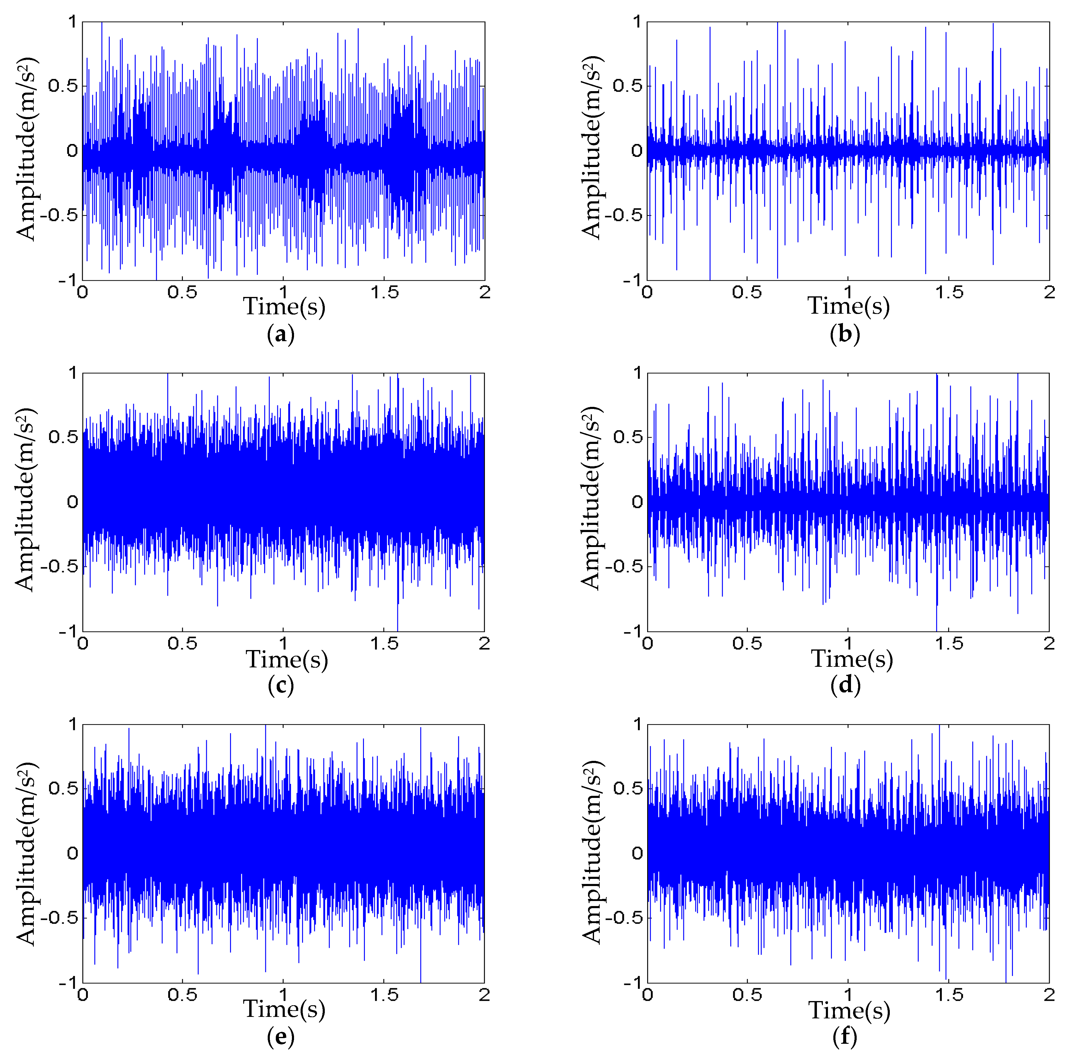
The six types of bearing faults of the measured signals include the IRF, ORF, and BF with three levels of fault diameters 0.007 inches and 0.021 inches, respectively. Just as the simulation signals, the length of each measured signal is 12,000 data points, which are used for testing SVM. The measured fault signals for testing samples are shown in Figure 7.
Similar to the FEM simulations for generating testing samples of six faults, each corresponding measured signal is normalized and divided into 40 sub-signals with 300 data points as length in the time domain, and the 16 corresponding time-domain indexes of each sub-signal are calculated. In this fault classification, all six types of fault training samples are all missed. The simulation signals are used to provide the faulty training samples, and the testing samples are all from the measured signals.
To distinguish the six faults numerically, they are labeled from 1 to 6, respectively. In the process of classification, the adjustable parameters of SVM are selected as ρ1 = 1.05 and C = 10 [27]. Based on the SVM toolkit trained by Franc et al. [38], the six types of faults in bearing are classified and the results are listed in Table 5. It shows that the fault classification accuracy ratios of outer ring, inner ring, and ball using the personalized diagnosis method are 90% (T1) and 92.5% (T2), 87.5% (T3) and 87.5% (T4), and 85%(T5) and 82.5% (T6), respectively. We can see that the classification accuracy ratios are not agreeable. To make a fair comparison, the classification accuracy using the measured signals alone (the training and testing samples are selected from the same measured signals) is also given using the same SVM with parameters ρ1 = 1.05 and C = 10. From Table 5, the relative errors of the present personalized diagnosis method with the measured signals alone are varying from 2.2 % to 12.8%. It notes that the relative errors of inner ring faults T3, T4, and ball fault T5 are a little bit large. The possible reason is the large measured noise of experimental test rigs of Bearing Data Centre at CWRU using the accelerometer mounted on the outer surface of bearing house far away from inner race and balls. In conclusion, the comparison investigations testify that the proposed personalized fault diagnosis method is feasible for judge the fault types of bearings.
Further, the possible way to improve the performance of the personalized diagnosis method is to do in-depth research on the construction of the simpler FEM models, high-performance FEM model updating, and updating more model parameters, and using transfer learning, etc.

4. Conclusions

For the application of machine learning methods in intelligent diagnosis of a mechanical system, sufficient fault training samples are the most basic and critical requirement. Based on the advantages of FEM simulation, the problem of lacking samples is solved by using FEM simulation, and the idea of personalized diagnosis based on FEM simulation driving machine learning is put forward. Specifically, a personalized fault diagnosis method based on FEM simulation driving SVM is proposed. The method is applied to diagnosis of the faults in a bearing, and the fault type are distinguished. In the experimental investigations using simulation signals to make up for the lack of faulty training samples, the classification accuracy of three faults located in outer ring, inner ring, and ball are 90% and 92.5%, 87.5% and 87.5%, and 85% and 82.5%, respectively. Finally, the classification results show that the present personalized fault diagnosis method is effective in identifying the faults in bearings. The proposed personalized fault diagnosis method based on FEM simulation driving machine learning can solve many problems, such as providing complete fault samples for various intelligent diagnosis, ensuring that the fault signal is pure without noise interference, etc.
Furthermore, the proposed method is worthy to be widely applied in complex mechanical systems for accurate fault detection.

Author Contributions

Conceptualization, J.X.; methodology, J.X.; software, X.L.; validation, X.L., J.X., and H.H.; formal analysis, X.L.; investigation, X.L.; resources, X.L.; data curation, X.L.; writing—original draft preparation, X.L.; writing—review and editing, J.X.; visualization, J.X.; supervision, J.X.; project administration, J.X.; funding acquisition, J.X. All authors have read and agree to the published version of the manuscript.

Funding

This work was funded in part by the National Natural Science Foundation of China under Grants U1909217 and U1709208, in part by the Zhejiang Special Support Program for High-level Personnel Recruitment of China under Grant 2018R52034, in part by the Wenzhou Key Innovation Project for Science and Technology of China under Grants 2018ZG023 and ZG2019018.

Conflicts of Interest

The authors declare no conflict of interest.

References

  1. Wang, D.; Miao, Q. Smoothness index-guided Bayesian inference for determining joint posterior probability distributions of anti-symmetric real Laplace wavelet parameters for identification of different bearing faults. J. Sound. Vib. 2015, 345, 250–266. [Google Scholar] [CrossRef]
  2. Zhao, R.; Yan, R.; Chen, Z.; Mao, K.; Wang, P.; Gao, R. Deep learning and its applications to machine health monitoring. Mech. Syst. Signal Pr. 2019, 115, 213–237. [Google Scholar] [CrossRef]
  3. Qin, Y.; Wang, X.; Zou, J.Q. The optimized deep belief networks with improved logistic Sigmoid units and their application in fault diagnosis for planetary gearboxes of wind turbines. IEEE T. Ind. Electron. 2019, 66, 3814–3824. [Google Scholar] [CrossRef]
  4. Wang, S.H.; Xiang, J.W.; Zhong, Y.T.; Zhou, Y.Q. Convolutional Neural Network-based Hidden Markov Models for Rolling Element Bearing Fault Identification. Knowl.-Based Syst. 2017, 144, 65–76. [Google Scholar] [CrossRef]
  5. Yang, B.; Lei, Y.G.; Jia, F.; Xing, S.B. An intelligent fault diagnosis approach based on transfer learning from laboratory bearings to locomotive bearings. Mech. Syst. Signal Pr. 2019, 122, 692–706. [Google Scholar] [CrossRef]
  6. Kumar, A.; Kumar, R. Time-frequency analysis and support vector machine in automatic detection of defect from vibration signal of centrifugal pump. Measurement 2017, 108, 119–133. [Google Scholar] [CrossRef]
  7. Wang, S.H.; Xiang, J.W.; Zhong, Y.T.; Tang, H.S. A data indicator-based deep belief networks to detect multiple faults in axial piston pumps. Mech. Syst. Signal Pr. 2018, 112, 154–170. [Google Scholar] [CrossRef]
  8. Wang, S.H.; Xiang, J.W. A minimum entropy deconvolution-enhanced convolutional neural networks for fault diagnosis of axial piston pumps. Soft Comput 2019, 1–15. [Google Scholar] [CrossRef]
  9. Kumar, A.; Kumar, R. Adaptive artificial intelligence for automatic identification of defect in the angular contact bearing. Neural. Comput. Appl. 2018, 29, 277–287. [Google Scholar] [CrossRef]
  10. Bregon, A.; Alonso-González, C.J.; Pulido, B. Integration of simulation and state observers for online fault detection of nonlinear continuous systems. IEEE Trans. Syst. Man Cy.-S. 2014, 44, 1553–1568. [Google Scholar] [CrossRef]
  11. Xiang, J.W.; Jiang, Z.S.; Chen, X.F. A class of wavelet-based Rayleigh-Euler beam element for analyzing rotating shafts. Shock Vib. 2011, 18, 447–458. [Google Scholar] [CrossRef]
  12. Xiang, J.W.; Long, J.Q.; Jiang, Z.S. A numerical study using Hermitian cubic spline wavelets for the analysis of shafts. Proc. Inst. Mech. Eng. 2010, 224, 1843–1851. [Google Scholar] [CrossRef]
  13. Xiang, J.W.; Zhong, Y.T. A novel personalized diagnosis methodology using numerical simulation and an intelligent method to detect faults in a shaft. Appl. Sci-Basel. 2016, 6, 414. [Google Scholar] [CrossRef] [Green Version]
  14. Wang, S.H.; Xiang, J.W.; Tang, H.S.; Liu, X.Y.; Zhong, Y.T. Minium entropy deconvolution based on simulation determined band pass fiter to detect faults in bearings of axial piston pumps. ISA Transaction 2018, 50, 599–608. [Google Scholar]
  15. Ren, W.X.; Chen, H.B. Finite element model updating in structural dynamics by using the response surface method. Eng. Struct. 2010, 32, 2455–2465. [Google Scholar] [CrossRef]
  16. Liu, B.; Ling, S.F. On the selection of informative wavelets for machinery diagnosis. Mech. Syst. Signal Pr. 1999, 13, 145–162. [Google Scholar] [CrossRef]
  17. Biswas, S.K.; Milanfar, P. One shot detection with laplacian object and fast matrix cosine similarity. IEEE T. Pattern Anal. 2016, 38, 546–562. [Google Scholar] [CrossRef]
  18. Chen, F.F.; Tang, B.P.; Song, T. Multi-fault diagnosis study on roller bearing based on multi-kernel support vector machine with chaotic particle swarm optimization. Measurement 2014, 47, 576–590. [Google Scholar] [CrossRef]
  19. Liu, W.Y.; Han, J.G.; Lu, X.N. A new gear fault feature extraction method based on hybrid time-frequency analysis. Neural Comput. Appl. 2014, 25, 387–392. [Google Scholar] [CrossRef]
  20. Liu, Z.; Cao, H.; Chen, X. Multi-fault classification based on wavelet SVM with PSO algorithm to analyze vibration signals from rolling element bearings. Neurocomputing 2013, 99, 399–410. [Google Scholar] [CrossRef]
  21. Hemez, F.M.; Doebling, S.W. Test-analysis correlation and finite element model updating for nonlinear transient dynamics. In Proceedings of the 17th International Modal Analysis Conference, Kissimmee, FL, USA, 1999; 3727, p. 1501. [Google Scholar]
  22. Link, M.; Weiland, M. Damage Identification by Multi-Model Updating in the Modal and in the Time Domain. Mech. Syst. Signal Process 2009, 23, 1734–1746. [Google Scholar] [CrossRef]
  23. Hasselman, T.K.; Anderson, M.C.; Gan, W.S. Principal components analysis for nonlinear model correlation, updating and uncertainty evaluation. In Proceedings of the 16th International Modal Analysis Conference, Santa Barbara, CA, USA, 1998; 3243, pp. 644–651. [Google Scholar]
  24. Sarin, H.; Kokkolaras, M.; Hulbert, G.; Papalambros, P. Comparing Time Histories for Validation of Simulation Models: Error Measures and Metrics. J. Dyn. Syst. 2010, 132, 173–179. [Google Scholar] [CrossRef] [Green Version]
  25. Zapico-Valle, J.L.; Alonso-Camblor, R. A new method for finite element model updating in structural dynamics. Mech. Syst. Signal Pr. 2010, 24, 2137–2159. [Google Scholar] [CrossRef]
  26. Kheir, N.A.; Holmes, W.M. Modeling and credibility of random ensembles. Simulation 1982, 38, 93–103. [Google Scholar] [CrossRef]
  27. Xiang, J.W.; Liang, M.; He, Y.M. Experimental investigation of frequency-based multi-damage detection for beams using support vector regression. Eng. Fract. Mech. 2014, 131, 257–268. [Google Scholar] [CrossRef]
  28. Case Western Reserve University. Bearing Data Center. Available online: http://csegroups.case.edu/bearingdatacenter/home (accessed on 26 October 2019).
  29. Hamrock, B.J.; Dowson, D. Ball bearing lubrication: The Elastohydrodynamics of Elliptical Contacts; Wiley & Sons: New York, NY, USA, 1982; pp. 279–281. [Google Scholar]
  30. Gupta, P.K. Advanced Dynamics of Rolling Elements; Springer: New York, NY, USA, 1986; pp. 203–209. [Google Scholar]
  31. Zhao, C.; Yu, X.; Huang, Q.; Ge, S.; Gao, X. Analysis on the load characteristics and coefficient of friction of angular contact ball bearing at high speed. Tribol. Int. 2015, 87, 50–56. [Google Scholar]
  32. Wei, J.; Gao, P.; Hu, X.L.; Sun, W. Effects of dynamic transmission errors and vibration stability in helical gears. J. Mech. Sci. Technol. 2014, 28, 2253–2262. [Google Scholar] [CrossRef]
  33. Zhao, M.M.; Ji, J.C. Dynamic analysis of wind turbine gearbox components. Energies 2016, 9, 110. [Google Scholar] [CrossRef] [Green Version]
  34. Al-Shyyab, A.; Kahraman, A. Non-linear dynamic analysis of a multi-mesh gear train using multi-term harmonic balance method: period-one motions. J. Sound Vib. 2005, 284, 151–172. [Google Scholar] [CrossRef]
  35. Chen, B.; Li, S.S.; Chen, J.; Lu, Y.X. The sources of damping in rolling element bearings under oscillating conditions. Lubr. Eng. 2013, 38, 62–66. [Google Scholar]
  36. Chen, S.Y.; Kung, C.; Liao, T.T. Dynamic analysis of a rotary hollow shaft with hot-fit part using contact elements with friction. T. Can. Soc. Mech. Eng. 2011, 35, 461–474. [Google Scholar] [CrossRef] [Green Version]
  37. Harris, T.A. Rolling Bearing Analysis, 3rd ed.; Wiley & Sons: London, UK, 1991. [Google Scholar]
  38. Franc, V.; Hlavác, V. Statistical Pattern Recognition Toolbox for Matlab; Center for Machine Perception, Czech Technical University: Prague, Czech Republic, 2004. [Google Scholar]
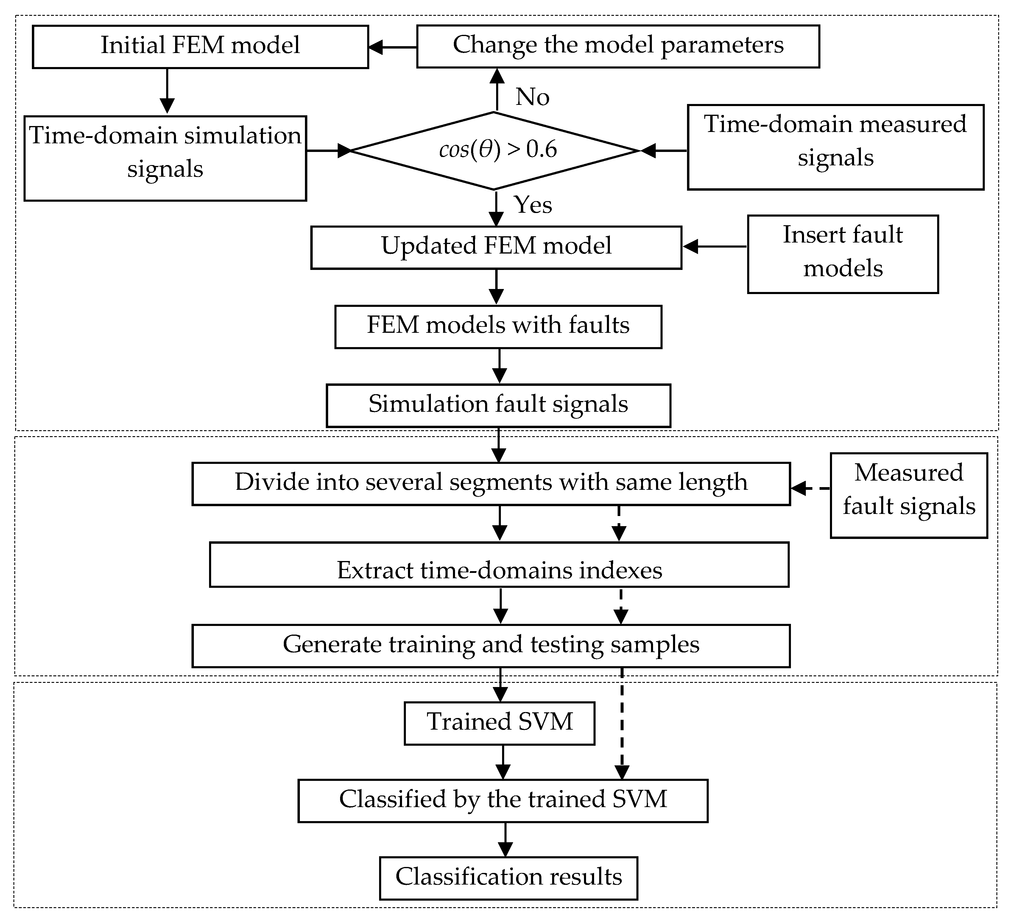
Figure 1. The flowchart of the personalized fault diagnosis method.
Sensors 20 00420 g001
Figure 2. The geometrical dimension and finite element method (FEM) model of a bearing: (a) the geometrical dimension and (b) the FEM model.
Sensors 20 00420 g002
Figure 3. The cosine similarity between measured and simulated signals in normal state.
Sensors 20 00420 g003
Figure 4. The comparison between measured and simulated signals in normal state.
Sensors 20 00420 g004
Figure 5. The geometry of faulty bearing: (a) Fault type T1; (b) Fault type T2; (c) Fault type T3; (d) Fault type T4; (e) Fault type T5; and (f) Fault type T6.
Sensors 20 00420 g005
Figure 6. The simulation signals with six types of faults: (a) Fault type T1; (b) Fault type T2; (c) Fault type T3; (d) Fault type T4; (e) Fault type T5; and (f) Fault type T6.
Sensors 20 00420 g006aSensors 20 00420 g006b
Figure 7. The measured signals with six types of faults: (a) Fault type T1 (b) Fault type T2, (c) Fault type T3, (d) Fault type T4, (e) Fault type T5, and (f) Fault type T6.
Sensors 20 00420 g007
Table 1. Sixteen indexes in time domain.
IndexEquationIndexEquation
Mean x m x m = i = 1 N x i / N Average amplitude x a v a x a v a = i = 1 N | x ( i ) | / N
Standard deviation x s t d x s t d = i = 1 N ( x ( i ) x m ) 2 / N Square root amplitude x s r a x s r a = ( i = 1 N | x ( i ) | / N ) 2
Variance x v a r x v a r = i = 1 N ( x i x m ) 2 / N Skewness x s k e x s k e = i = 1 N ( x ( i ) x m ) 3 / N
Peak x P x P = m a x | x ( i ) | Kurtosis x k u r x k u r = i = 1 N ( x ( i ) x m ) 4 / N x s t d 4
Maximum x m a x x m a x = m a x ( x ( i ) ) Shape factor S F S F = x r m s / ( i = 1 N | x ( i ) | / N )
Minimum x m i n x m i n = m i n ( x ( i ) ) Impulse factor I F I F = x P / ( i = 1 N | x ( i ) | / N )
Peak to peak x p p x p p = m a x ( x ( i ) ) m i n ( x ( i ) ) Peak factor P F P F = x P / x r m s
Root mean square x r m s x r m s = i = 1 N ( x i ) 2 / N Clearance indicator C I C I = x m a x / ( i = 1 N | x ( i ) | / N ) 2
x is the data; N is the number of data points.
Table 2. The element size of bearing.
ComponentElement Size (mm)
Outer ring1
Inner ring1
Ball1
Cage0.5
Shaft2
Bearing seat2
Table 3. Contact parameters and loading parameters for the FEM model.
Contact ParametersValueLoading ParametersValue
FKN0.12Fg500 N
f10.02Fe0.12 MPa
f20.016n1797 rpm
λ 0.02Fro0.5 MPa
Table 4. The experimental design and cosine similarity value of model parameter updating.
cos(θ).Fe (MPa)
00.040.080.120.160.2
Fg (N) 1000.2020.2680.3940.5050.4030.374
2000.1930.2920.4630.5590.4460.351
3000.1510.2550.4120.4980.5010.306
4000.2060.3110.4550.5810.4550.364
5000.2230.3510.5010.6180.4510.411
6000.1690.2710.5040.6010.5070.403
7000.2010.3360.5030.4990.4730.418
8000.2030.2270.4720.5490.4370.372
9000.1740.2940.4180.5170.4220.393
10000.1610.2580.3580.4580.4280.358
Table 5. The classification results using the proposed method (16 indexes) and measured fault signals alone.
Fault TypeTraining SamplesTesting SamplesFaults LabelsClassification Accuracy Using the Present Method (%)Classification Accuracy Using the Measured Signals Alone (%)Relative Error (%)
T14040190%92%2.2
T24040292.5%95%2.6
T34040387.5%95%7.9
T44040487.5%90%7.9
T54040585%97.5%12.8
T64040682.5%87.5%5.7