An Extended Kalman Filter and Back Propagation Neural Network Algorithm Positioning Method Based on Anti-lock Brake Sensor and Global Navigation Satellite System Information

Abstract
1. Introduction
2. Positioning Scheme Based on ABS Sensor and GNSS Information Fusion
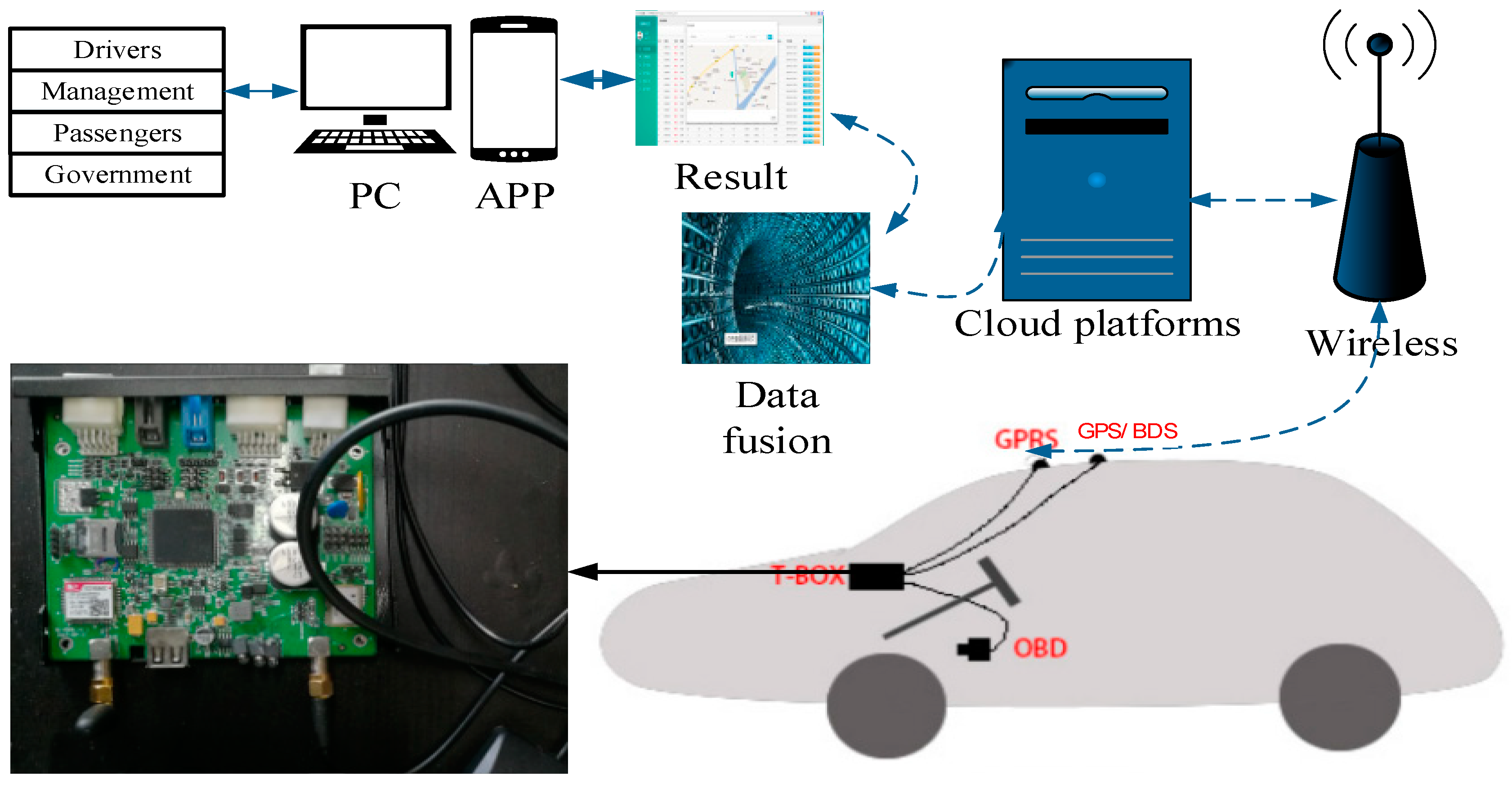
2.1. Fusion Positioning System
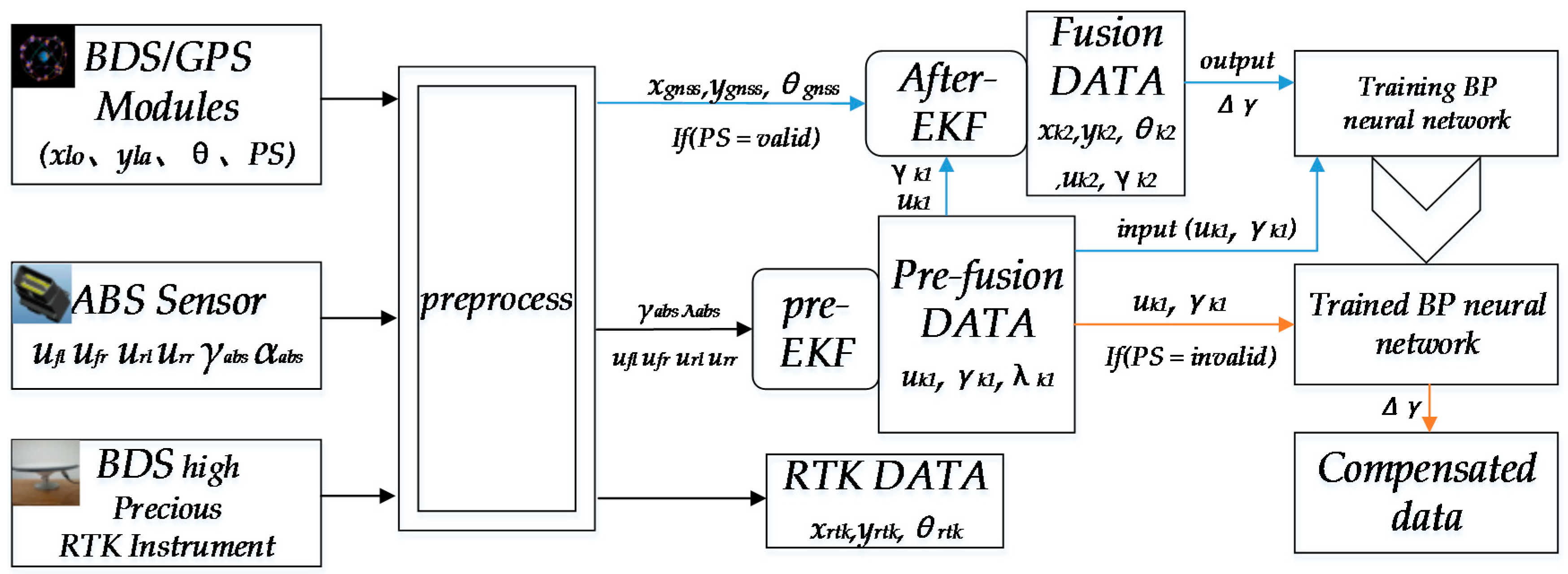
2.2. Fusion Positioning Method
3. Dual Kalman Filtering-Based Positioning Research
3.1. Fusion Positioning System
3.2. After-EKF Model
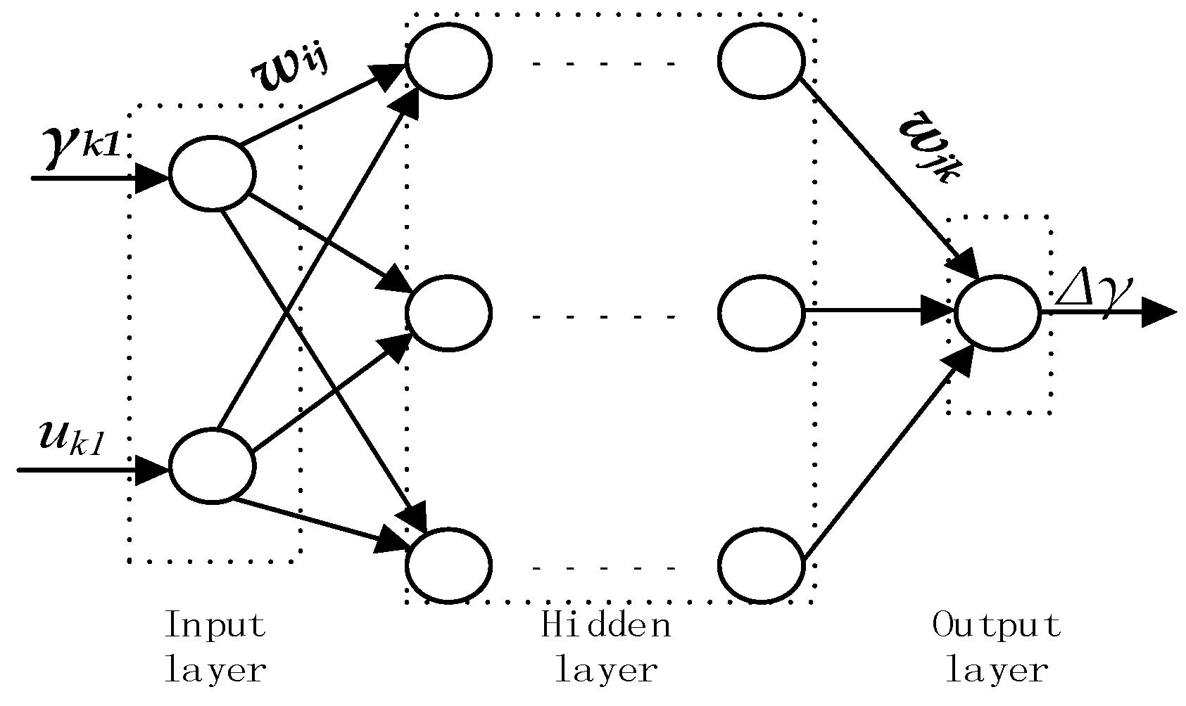
4. Study of Positioning Method Based on BP Neural Network
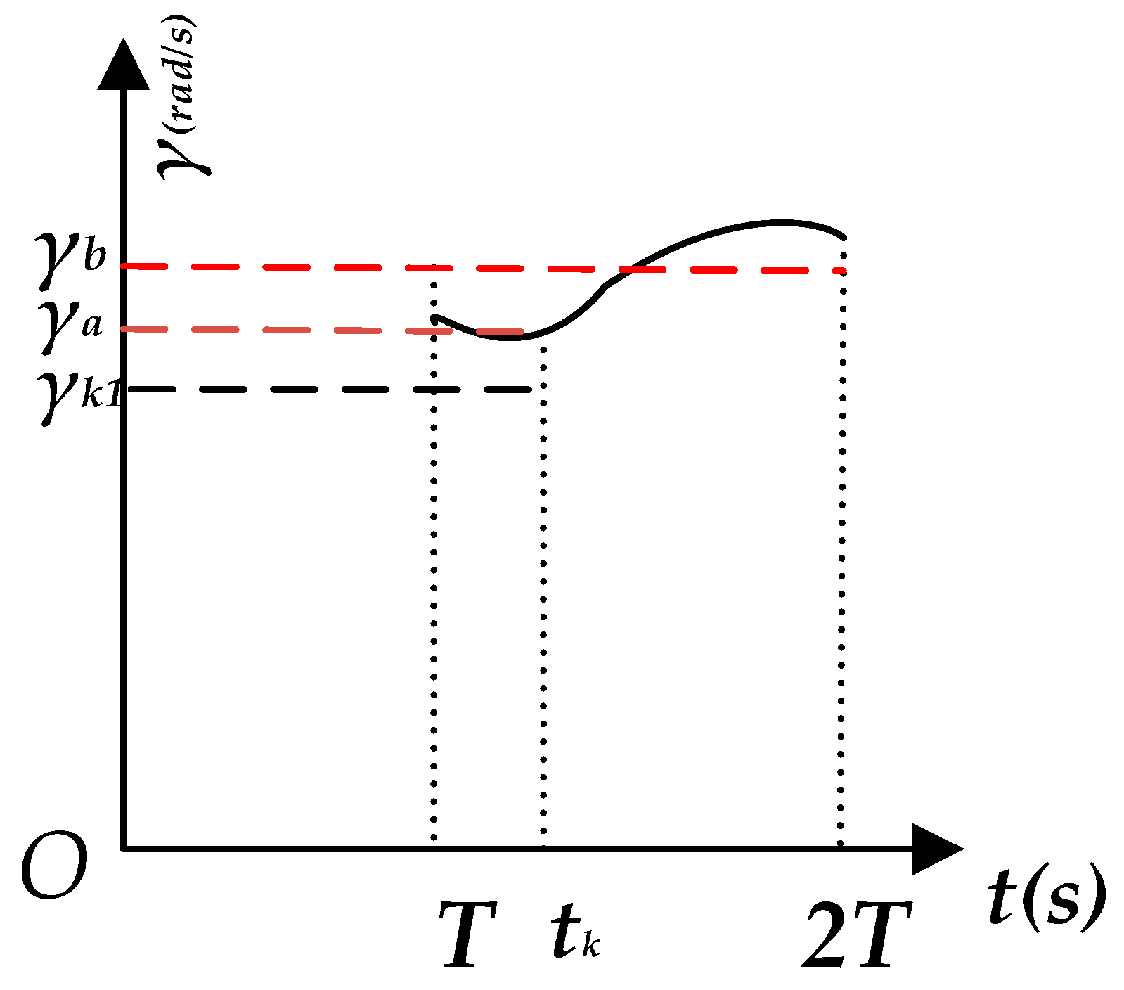
- : actual value of corresponding to time
- : expected value referring to the average value of from time T to time 2T
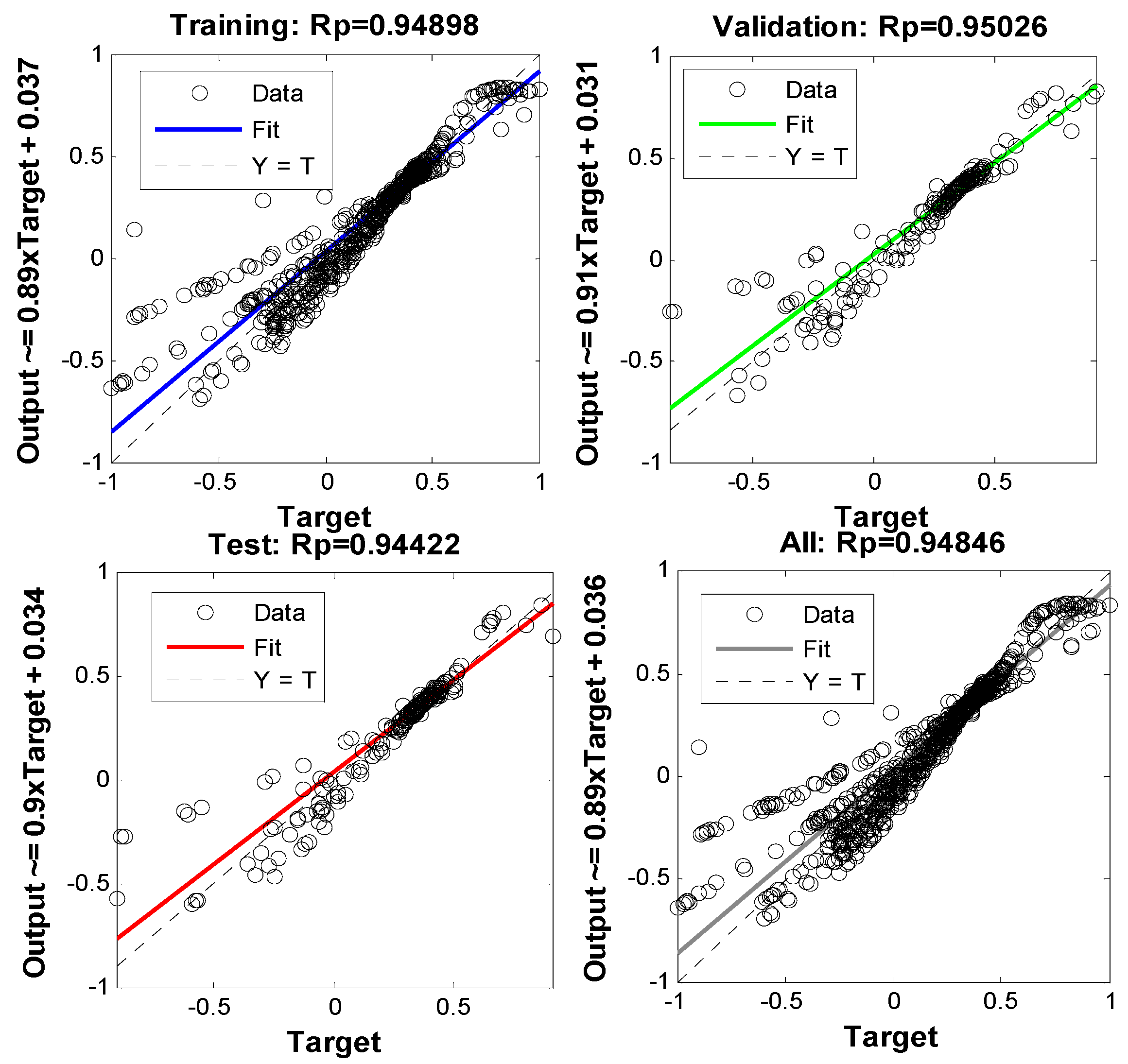
4.1. BP Neural Network Model
4.2. Determination of the BP Neural Network Structure
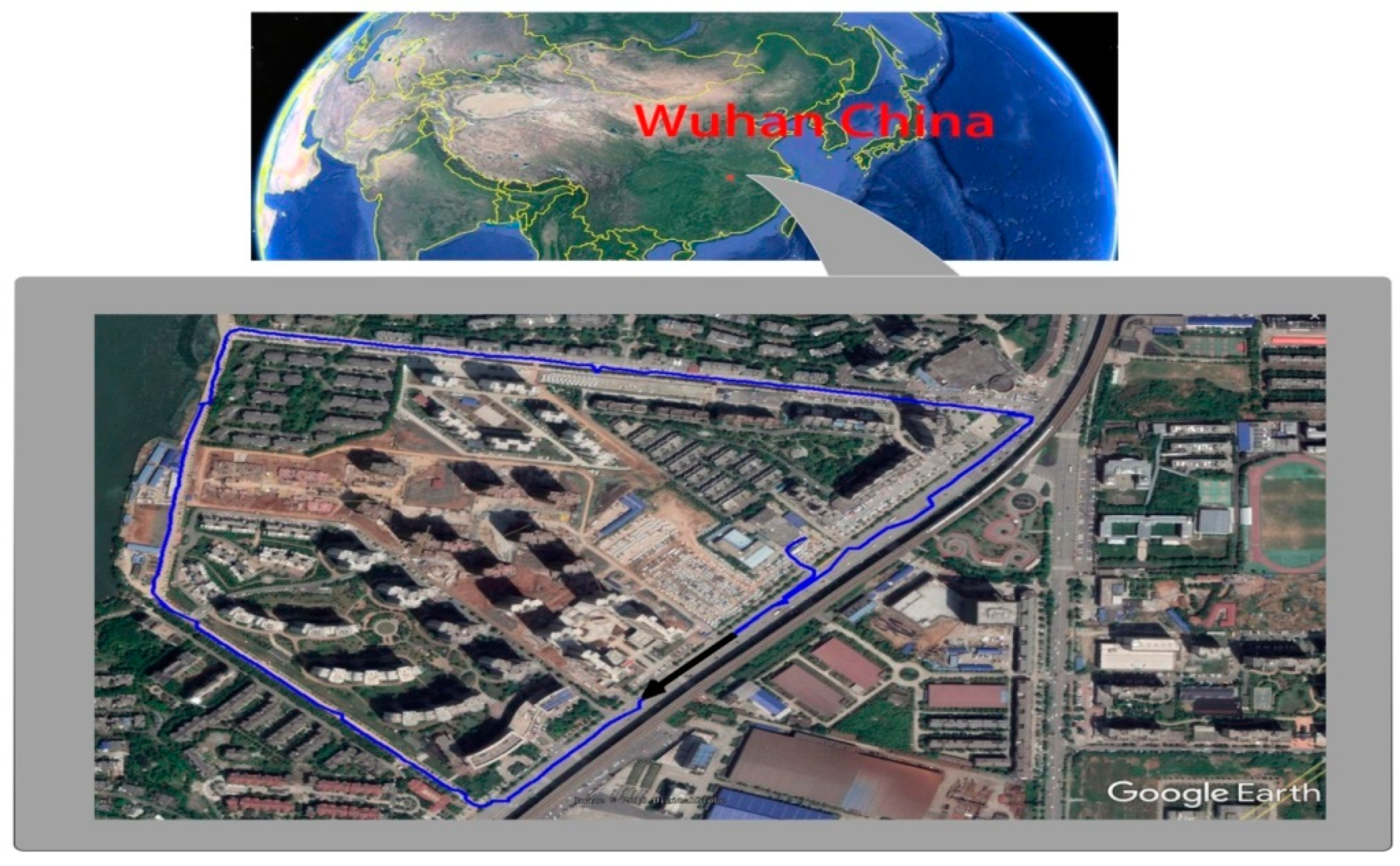
5. Experimental Study and Analysis of Results
5.1. Testing Program
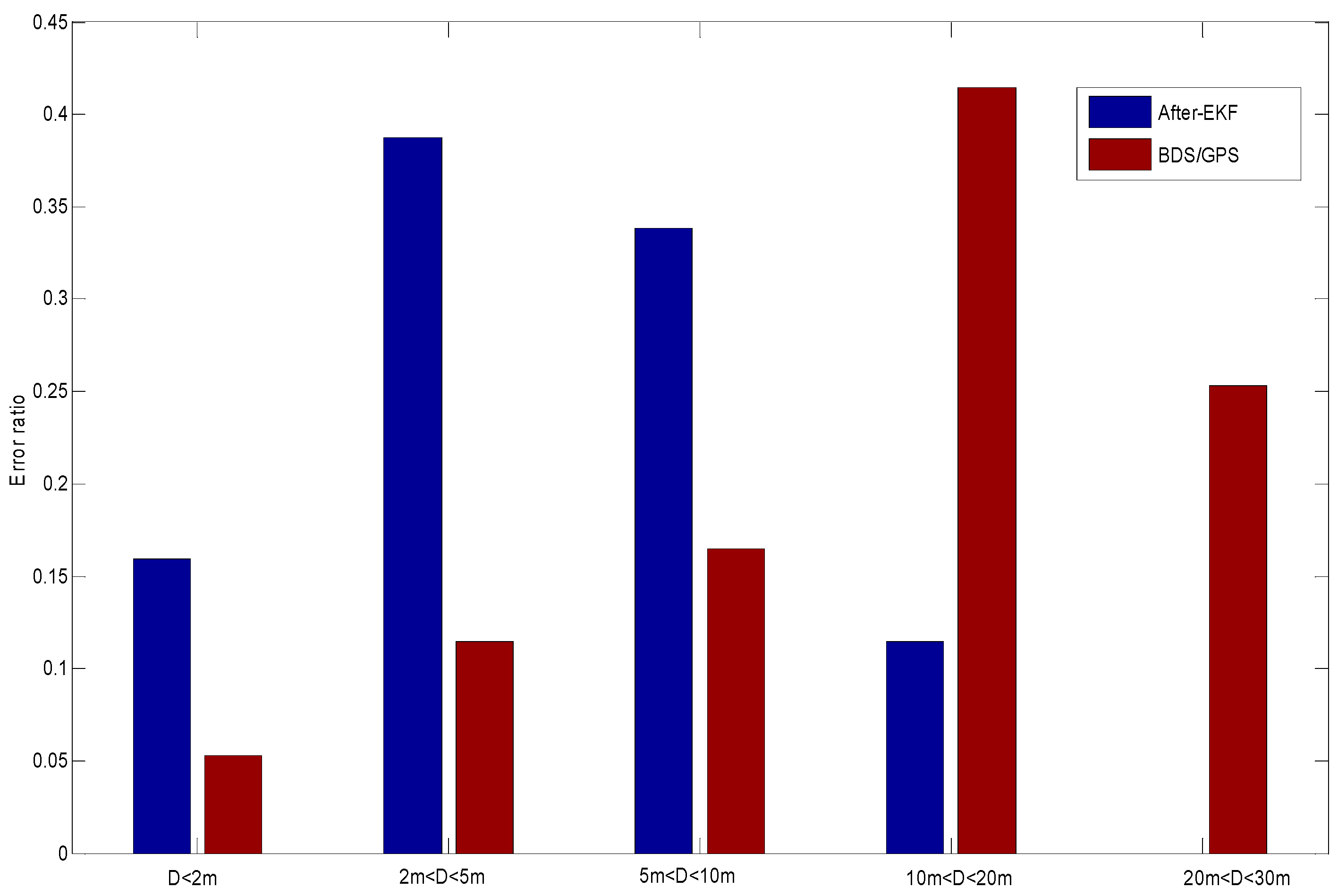
5.2. Analysis of Positioning Effects in Case of GNSS Positioning Status Being Valid
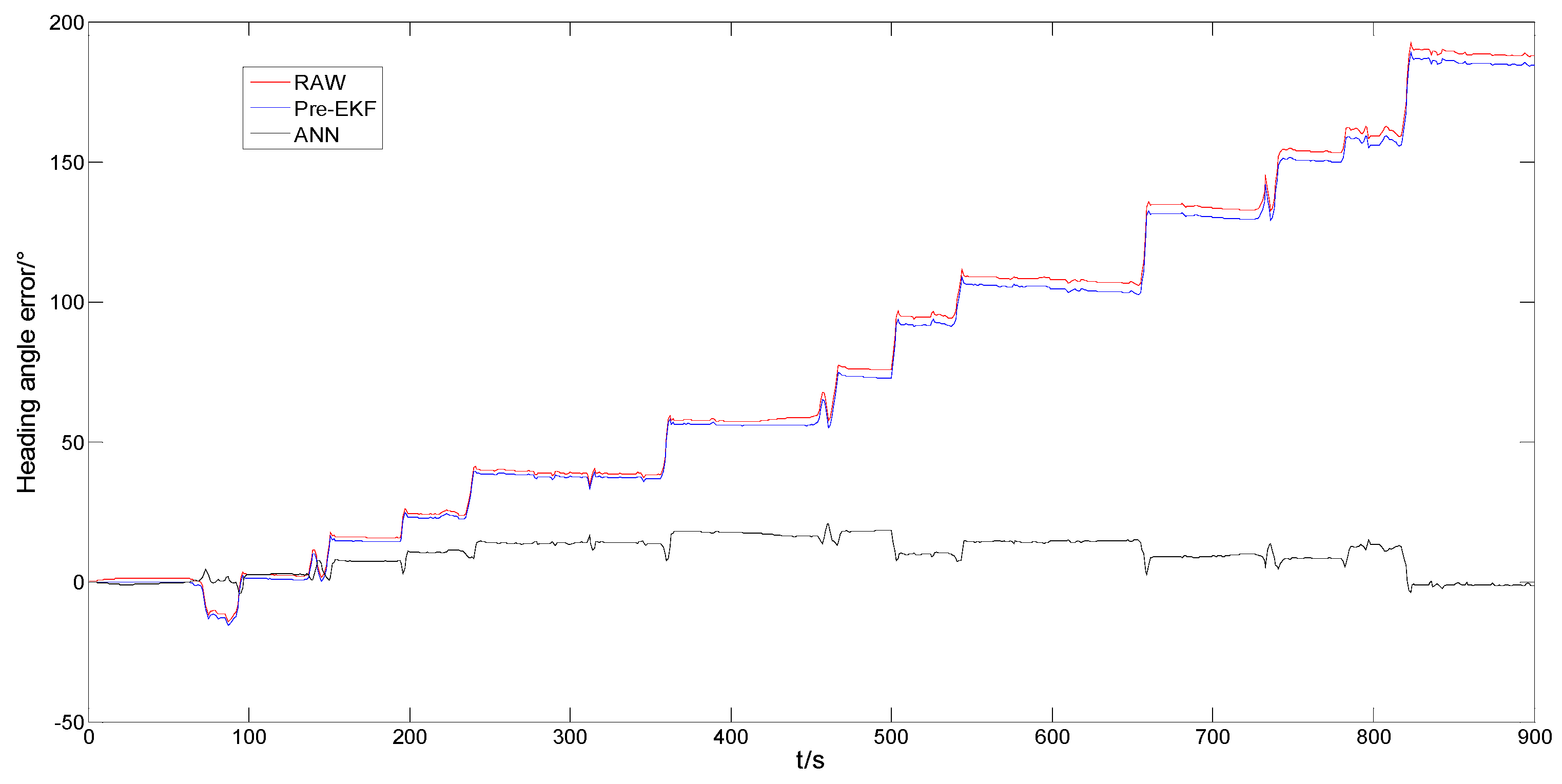
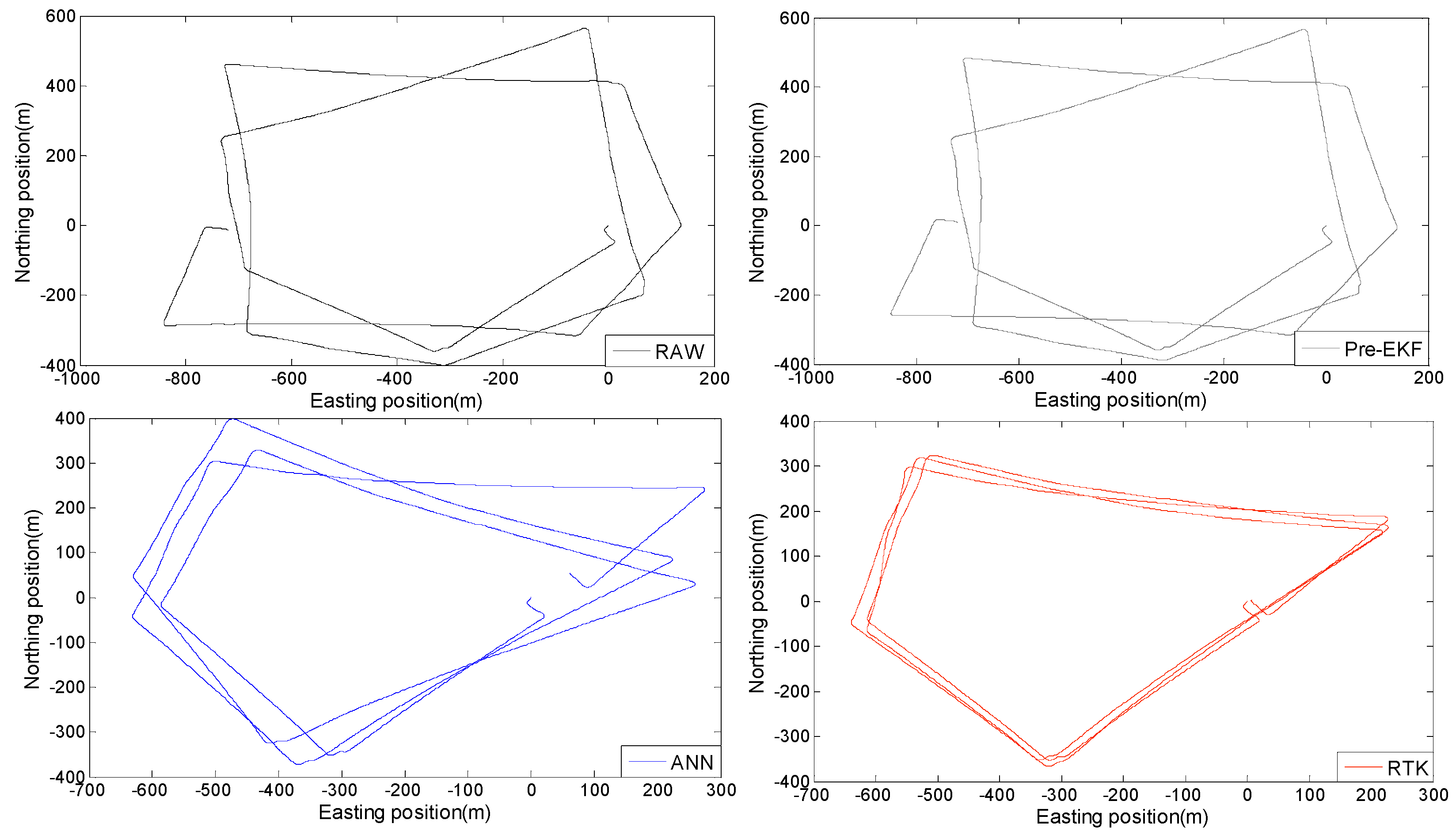
5.3. Analysis of Positioning Effects in Case of Invalid of GNSS Positioning Status
- (1)
- 30 min sample data;
- (2)
- 15 min performance display data.
6. Conclusions and Outlook
Author Contributions
Funding
Acknowledgements
Conflicts of Interest
References
- Karagiannis, G.; Altintas, O.; Ekici, E.; Heijenk, G.; Jarupan, B.; Lin, K.; Weil, T. Vehicular Networking: A Survey and Tutorial on Requirements, Architectures, Challenges, Standards and Solutions. IEEE Commun. Surv. Tutor. 2011, 13, 584–616. [Google Scholar] [CrossRef]
- Hadiwardoyo, S.A.; Patra, S.; Calafate, C.T.; Cano, J.-C.; Manzoni, P. An Intelligent Transportation System Application for Smartphones Based on Vehicle Position Advertising and Route Sharing in Vehicular Ad-Hoc Networks. J. Comput. Sci. Technol. 2018, 33, 249–262. [Google Scholar] [CrossRef]
- Cucinotta, F.; Costa, D. Telematic Box Device for Motor Vehicles. EP3021290A1, 18 May 2016. [Google Scholar]
- Reese, K.J.; Jones, A.; Turner, M. Inline GPS Receiver Module. U.S. Patent 20110068974A1, 24 March 2011. [Google Scholar]
- Dong, D.; Wang, M.; Chen, W.; Zeng, Z.; Song, L.; Zhang, Q.; Cai, M.; Cheng, Y.; Lv, J. Mitigation of multipath effect in GNSS short baseline positioning by the multipath hemispherical map. J. Geod. 2016, 90, 255–262. [Google Scholar] [CrossRef]
- Cheng, Y.-M. Method and Apparatus for Positioning an Unmanned Vehicle in Proximity to a Person or an Object Based Jointly on Placement Policies and Probability of Successful Placement. U.S. Patent 20150057917A1, 26 February 2015. [Google Scholar]
- Song, J.H.; Jee, G.I. Performance Enhancement of Land Vehicle Positioning Using Multiple GPS Receivers in an Urban Area. Sensors 2016, 16, 1688. [Google Scholar] [CrossRef] [PubMed]
- Lu, Z.; Wang, J.; Ba, B.; Wang, D. A novel direct position determination algorithm for orthogonal frequency division multiplexing signals based on the time and angle of arrival. IEEE Access 2017, 5, 25312–25321. [Google Scholar] [CrossRef]
- Zhang, H.M.; Deng, Z.L. UKF Method for Land Vehicle Integrated Navigation Systems. J. Chin. Inertial Technol. 2004, 12, 20–23. [Google Scholar]
- Donovan, G.T. Position Error Correction for an Autonomous Underwater Vehicle Inertial Navigation System (INS) Using a Particle Filter. IEEE J. Ocean. Eng. 2012, 37, 431–445. [Google Scholar] [CrossRef]
- Yun, X.; Bachmann, E.R.; Mcghee, R.B.; Whalen, R.H.; Roberts, R.L.; Knapp, R.G.; Healey, A.J.; Zyda, M.J. Testing and evaluation of an integrated GPS/INS system for small AUV navigation. IEEE J. Ocean. Eng. 1999, 24, 396–404. [Google Scholar] [CrossRef]
- Upadhyay, T.N.; Cotterill, S.; Deaton, A.W. Autonomous GPS/INS navigation experiment for space transfer vehicle. IEEE Trans. Aerosp. Electron. Syst. 1991, 29, 772–785. [Google Scholar] [CrossRef]
- Malleswaran, M.; Vaidehi, V.; Mohankumar, M. A hybrid approach for GPS/INS integration using Kalman filter and IDNN. In Proceedings of the Third International Conference on Advanced Computing, Chennai, India, 14–16 December 2011. [Google Scholar]
- Malleswaran, M.; Vaidehi, V.; Saravanaselvan, A. Performance Analysis of Various Artificial Intelligent Neural Networks for GPS/INS Integration. Eng. Appl. Artif. Intell. 2013, 27, 367–407. [Google Scholar] [CrossRef]
- Huang, J.Y.; Huang, Z.Y.; Chen, K.H. Combining low-cost Inertial Measurement Unit (IMU) and deep learning algorithm for predicting vehicle attitude. In Proceedings of the IEEE Conference on Dependable and Secure Computing, Taipei, Taiwan, 7–10 August 2017. [Google Scholar]
- Hu, B.; Dixon, P.C.; Jacobs, J.V.; Jacobs, J.V.; Dennerlein, J.T.; Schiffman, J.M. Machine learning algorithms based on signals from a single wearable inertial sensor can detect surface- and age-related differences in walking. J. Biomech. 2018, 71, 37–42. [Google Scholar] [CrossRef] [PubMed]
- Quddus, M.A.; Ochieng, W.Y.; Noland, R.B. Current map-matching algorithms for transport applications: State-of-the art and future research directions. Transp. Res. Part C Emerg. Technol. 2007, 15, 312–328. [Google Scholar] [CrossRef]
- Attia, M.; Moussa, A.; El-Sheimy, N. Updating Integrated GPS/INS Systems with Map Matching for Car Navigation Applications. In Proceedings of the 24th International Technical Meeting of The Satellite Division of the Institute of Navigation (ION GNSS 2011), Portland, OR, USA, 1 January 2011. [Google Scholar]
- Kim, S.; Kim, J.H. Adaptive fuzzy-network-based C-measure map-matching algorithm for car navigation system. IEEE Trans. Ind. Electron. 2001, 48, 432–441. [Google Scholar]
- Alam, N.; Kealy, A.; Dempster, A.G. An INS-Aided Tight Integration Approach for Relative Positioning Enhancement in VANETs. IEEE Trans. Intell. Transp. Syst. 2013, 14, 1992–1996. [Google Scholar] [CrossRef]
- Rakouth, H.; Alexander, P.; Brown, A.; Brown, A., Jr.; Kosiak, W.; Fukushima, M.; Ghosh, L.; Hedges, C.; Kong, H.; Kopetzki, S.; Siripurapu, R.; et al. V2X Communication Technology: Field Experience and Comparative Analysis. In Lecture Notes in Electrical Engineering, Proceedings of the FISITA 2012 World Automotive Congress, Beijing, China, 27–30 November 2012; Springer: Berlin/Heidelberg, Germany, 2013. [Google Scholar]
- Khattab, A.; Fahmy, Y.A.; Wahab, A.A. High Accuracy GPS-Free Vehicle Localization Framework via an INS-Assisted Single RSU. Int. J. Distrib. Sens. Netw. 2015, 2015, 1–16. [Google Scholar] [CrossRef]
- Wahab, A.A.; Khattab, A.; Fahmy, Y.A. Two-way TOA with limited dead reckoning for GPS-free vehicle localization using single RSU. ITS Telecommun. 2013, 12, 244–249. [Google Scholar]
- Chi, J.; Do, S.; Park, S. Traffic flow-based roadside unit allocation strategy for VANET. In Proceedings of the International Conference on Big Data and Smart Computing (BigComp), Hong Kong, China, 18–20 January 2016. [Google Scholar]
- Melendez-Pastor, C.; Ruiz-Gonzalez, R.; Gomez-Gil, J. A data fusion system of GNSS data and on-vehicle sensors data for improving car positioning precision in urban environments. Expert Syst. Appl. 2017, 80, 28–38. [Google Scholar] [CrossRef]
- Grewal, M.S.; Weill, L.R.; Andrews, A.P. Global positioning systems, inertial navigation, and integration. Wiley Interdiscip. Rev. Comput. Stat. 2011, 3, 383–384. [Google Scholar] [CrossRef]
- Mourikis, A.I.; Roumeliotis, S.I. Analysis of Positioning Uncertainty in Simultaneous Localization and Mapping (SLAM). IROS 2004, 1, 13–20. [Google Scholar]
- Trehard, G.; Pollard, E.; Bradai, B.; Nashashibi, F. On line mapping and global positioning for autonomous driving in urban environment based on evidential SLAM. Proceedings of IEEE Intelligent Vehicles Symposium (IV), Seoul, Korea, 28 June–1 July 2015; pp. 814–819. [Google Scholar]
- Lee, C.-H.; Tahk, M.-J. Unmanned Aerial Vehicle Recovery Using a Simultaneous Localization and Mapping Algorithm without the Aid of Global Positioning System. Int. J. Aeronaut. Space Sci. 2010, 11, 98–109. [Google Scholar] [CrossRef]
- Feng, G.S.; Feng, L.S.; Jia, S.M.; Wang, H.H.; Zheng, M.J. Development of On-board Diagnostic System Based on Wireless Network. Veh. Eng. 2013, 1. [Google Scholar] [CrossRef]
- Jimenez, A.R.; Seco, F.; Prieto, C.; Guevara, J. A comparison of pedestrian dead-reckoning algorithms using a low-cost mems IMU. In Proceedings of the IEEE International Symposium on Intelligent Signal Processing, Budapest, Hungary, 26–28 August 2009. [Google Scholar] [CrossRef]
- Tamaddoni, S.H.; Taheri, S.; Ahmadian, M. Optimal preview game theory approach to vehicle stability controller design. Veh. Syst. Dyn. 2011, 49, 1967–1979. [Google Scholar] [CrossRef]
- Dixon, J.C. The Equations of Lateral Motion of the Two Degree-of-Freedom Model of the Four-Wheeled Road Vehicle. SAE Tech. Pap. 1990, 901732. [Google Scholar] [CrossRef]


| Parameters | Parameters | ||
|---|---|---|---|
| u | vehicle speed | γ | heading angle speed |
| xlo | longitude of BDS | yla | latitude of BDS |
| xrtk | longitude of RTK | yrtk | latitude of RTK |
| θ | heading angle | PS | positioning valid status |
| rotation angle of the steering wheel | heading angle speed | ||
| speed of left front-wheel | speed of right front-wheel | ||
| speed of left rear-wheel | speed of right rear-wheel | ||
| vehicle speed | heading angle speed | ||
| tangent value of front-wheel steering angle | |||
| relative latitude-conversion | relative longitude-conversion | ||
| heading angle | vehicle speed | ||
| heading angle speed | Δγ | heading angle speed error | |
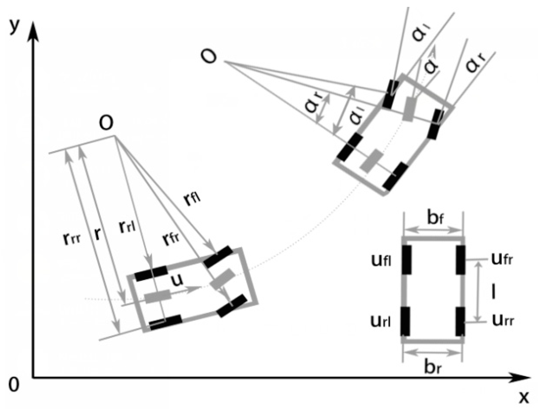
| Parameters | Parameters | ||
|---|---|---|---|
| Front-wheel virtual steering angle | Tangent value of front-wheel steering angle | ||
| l | Vehicle wheelbase | r | Steering radius of the vehicle |
| bf | Front-wheel track | br | Rear-wheel track |
| Deflection angle of the left front-wheel | Deflection angle of the right front-wheel | ||
| rfl | Left front-wheel | rfr | Right front-wheel |
| rrl | Left rear-wheel | rrr | Right rear-wheel |
| Parameters | Values |
|---|---|
| Front track | 1.496 m |
| Rear track | 1.490 m |
| Wheelbase | 2.550 m |
| Test speed | ~40 km/h |
© 2018 by the authors. Licensee MDPI, Basel, Switzerland. This article is an open access article distributed under the terms and conditions of the Creative Commons Attribution (CC BY) license (http://creativecommons.org/licenses/by/4.0/).
Share and Cite
Hu, J.; Wu, Z.; Qin, X.; Geng, H.; Gao, Z. An Extended Kalman Filter and Back Propagation Neural Network Algorithm Positioning Method Based on Anti-lock Brake Sensor and Global Navigation Satellite System Information. Sensors 2018, 18, 2753. https://doi.org/10.3390/s18092753
Hu J, Wu Z, Qin X, Geng H, Gao Z. An Extended Kalman Filter and Back Propagation Neural Network Algorithm Positioning Method Based on Anti-lock Brake Sensor and Global Navigation Satellite System Information. Sensors. 2018; 18(9):2753. https://doi.org/10.3390/s18092753
Chicago/Turabian StyleHu, Jie, Zhongli Wu, Xiongzhen Qin, Huangzheng Geng, and Zhangbin Gao. 2018. "An Extended Kalman Filter and Back Propagation Neural Network Algorithm Positioning Method Based on Anti-lock Brake Sensor and Global Navigation Satellite System Information" Sensors 18, no. 9: 2753. https://doi.org/10.3390/s18092753
APA StyleHu, J., Wu, Z., Qin, X., Geng, H., & Gao, Z. (2018). An Extended Kalman Filter and Back Propagation Neural Network Algorithm Positioning Method Based on Anti-lock Brake Sensor and Global Navigation Satellite System Information. Sensors, 18(9), 2753. https://doi.org/10.3390/s18092753