On Target Localization Using Combined RSS and AoA Measurements


Abstract
:1. Introduction
1.1. Motivation
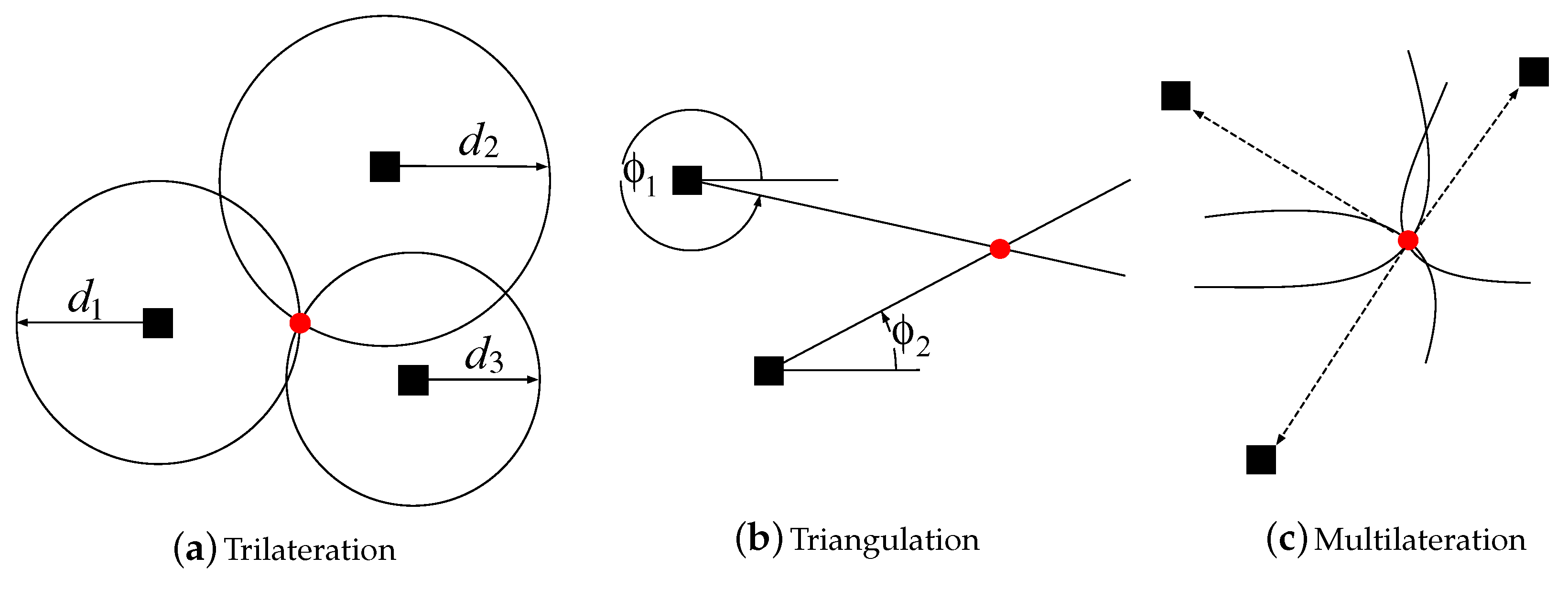
1.2. Related Work
2. Hybrid RSS/AoA Localization
2.1. Problem Formulation
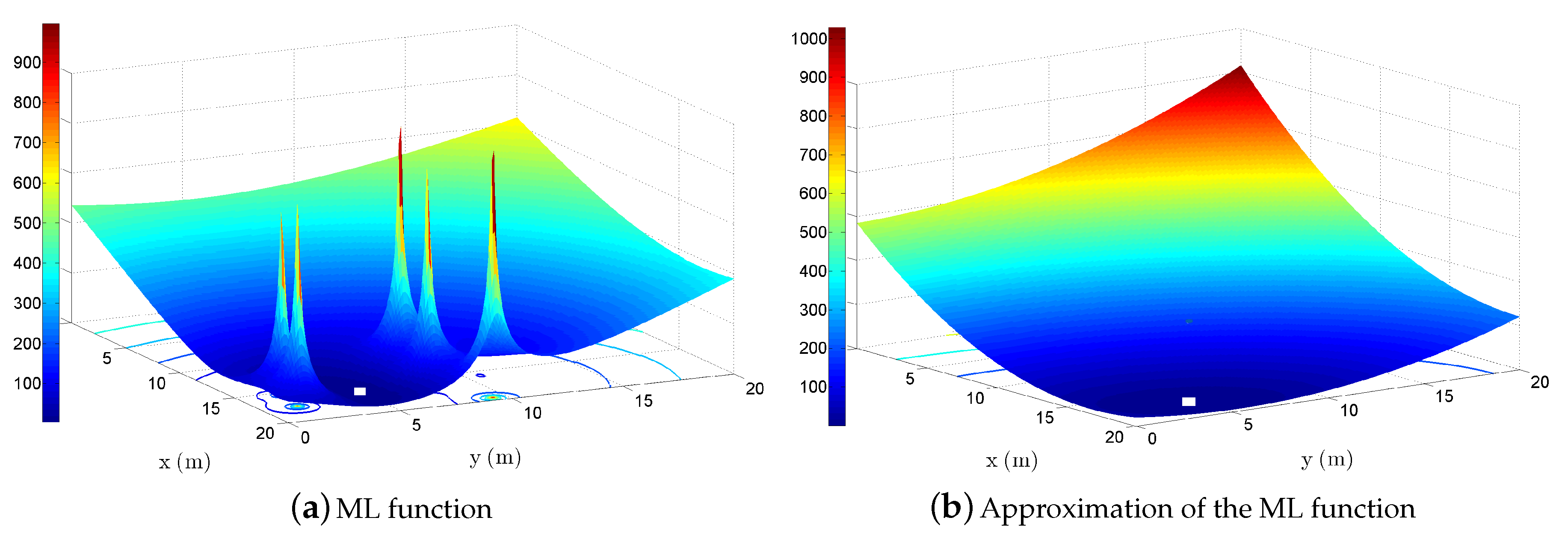
2.2. SDP Estimator
2.3. SOCP Estimator
2.4. SR-WLS Estimator
2.5. WLS Estimator
2.6. LS Estimator
2.7. WLLS Estimator
3. Complexity Analysis
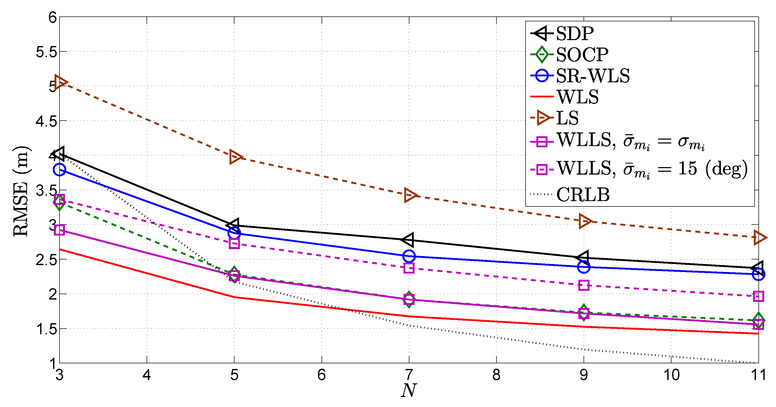
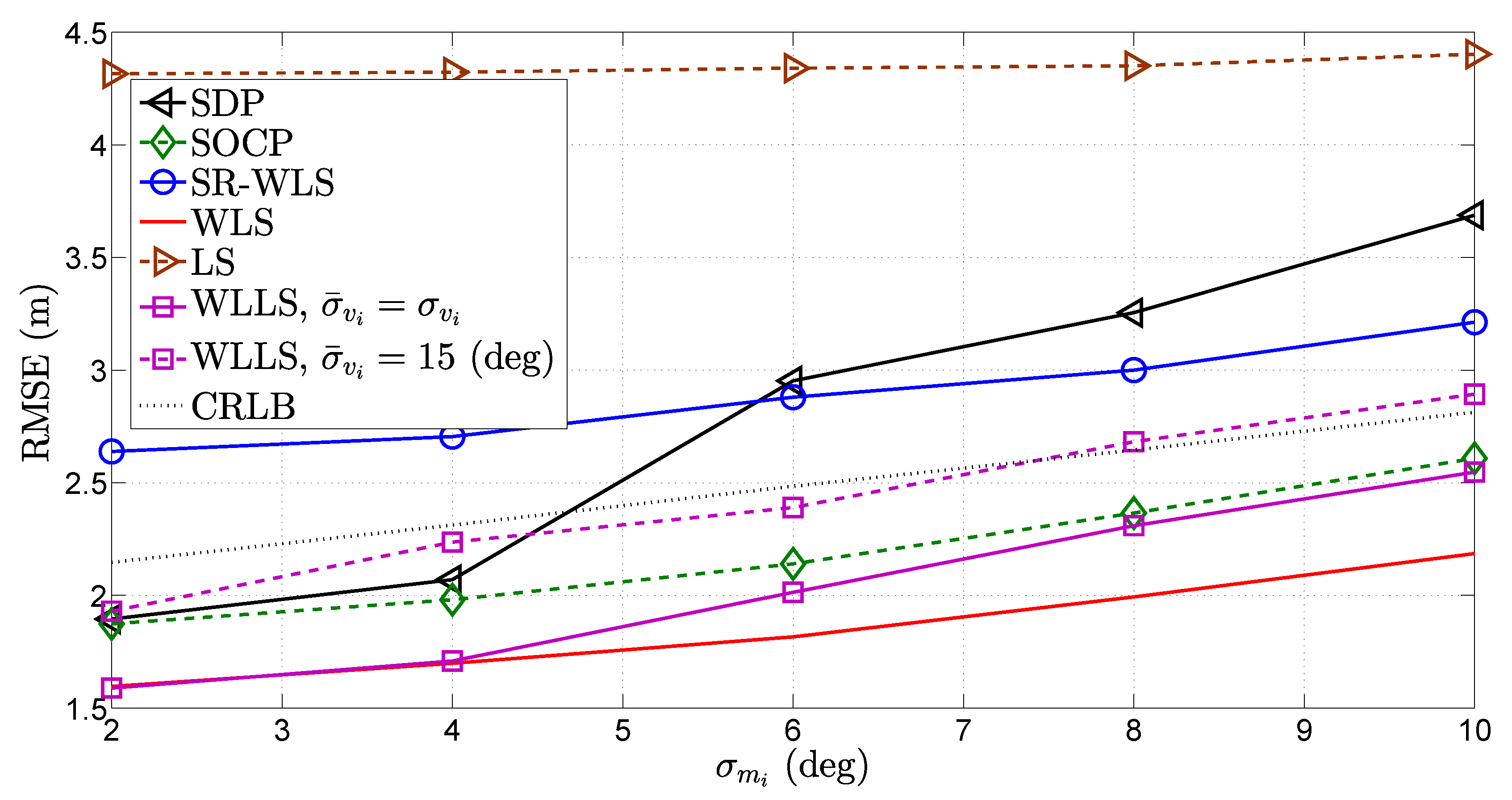
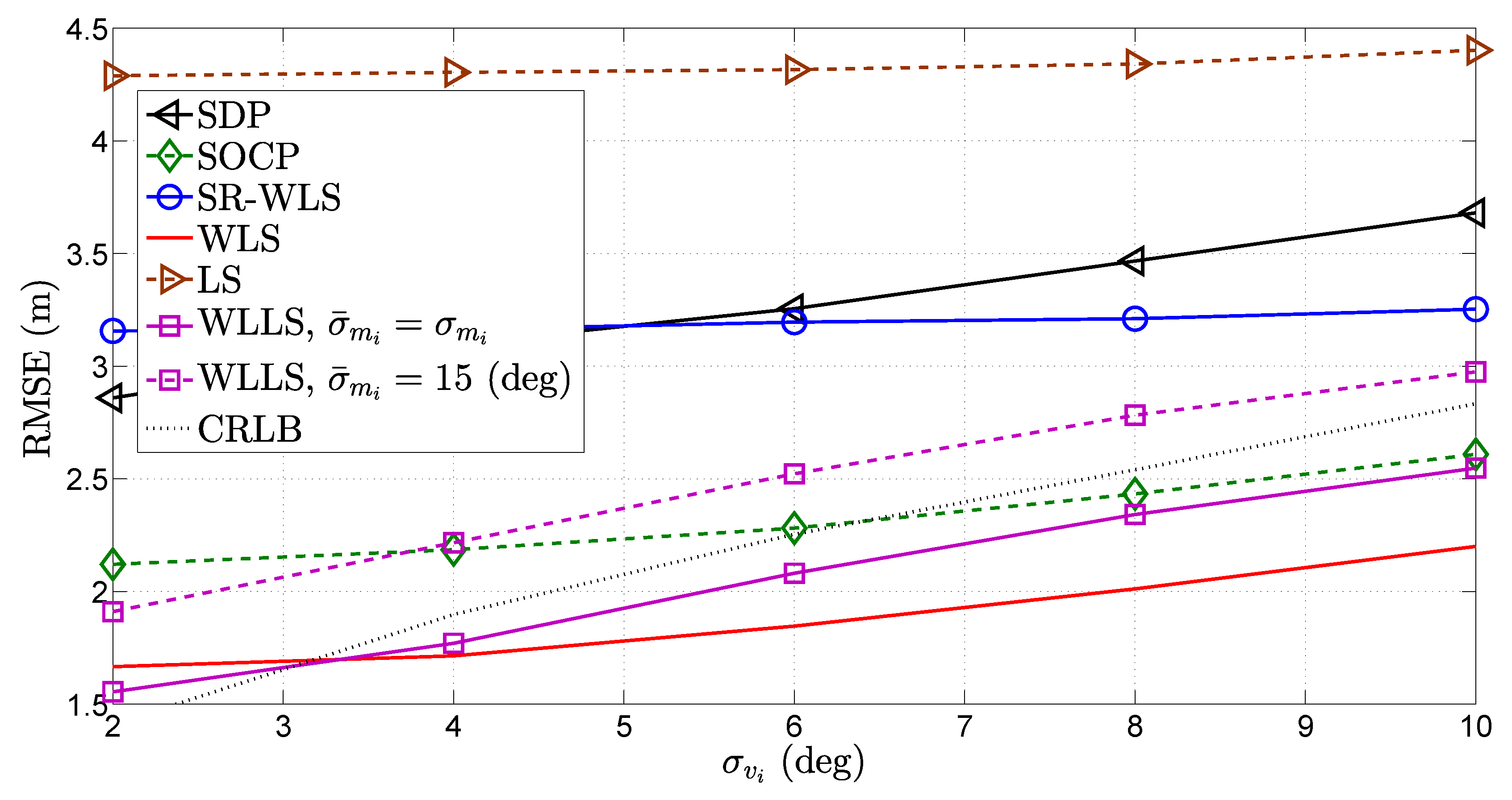
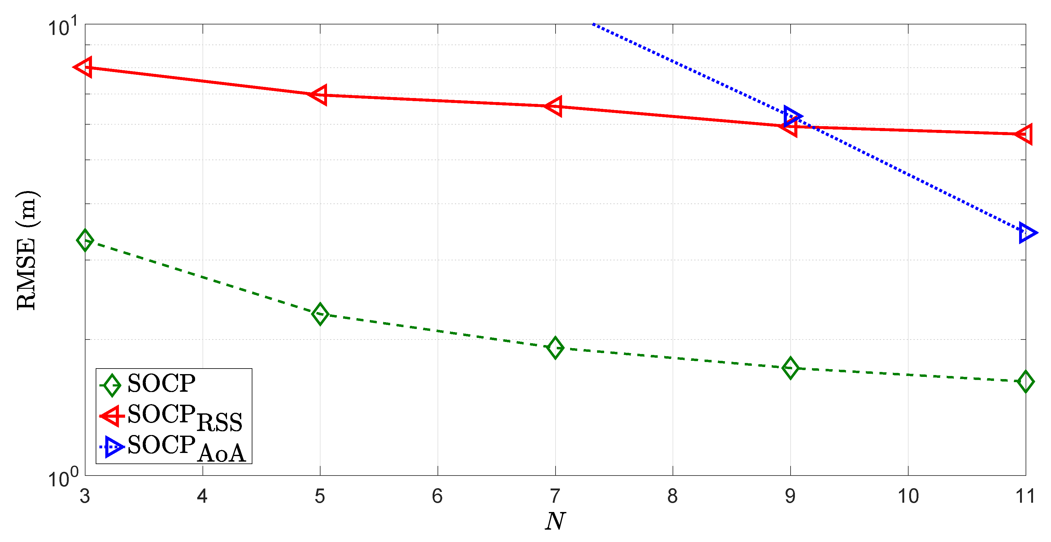
4. Performance Results
5. Conclusions and Future Work
5.1. Conclusions
5.2. Future Work
Acknowledgments
Author Contributions
Conflicts of Interest
Appendix A. Derivation of the Covariance Matrix
Appendix B. CRLB Derivation for RSS-AoA Localization
References
- Patwari, N. Location Estimation in Sensor Networks. Ph.D. Thesis, University of Michigan, Ann Arbor, MI, USA, 2005. [Google Scholar]
- Rongbai, Z.; Guohua, C. Research on Major Hazard Installations Monitoring System Based on WSN. In Proceedings of the International Conference on Future Computer & Communication, ICFCC, Wuhan, China, 21–24 May 2010; pp. 741–745. [Google Scholar]
- Dai, Z.; Wang, S.; Yan, Z. BSHM-WSN: A Wireless Sensor Network for Bridge Structure Health Monitoring. In Proceedings of the International Conference on Modelling, Identification & Control (ICMIC), Wuhan, China, 24–26 June 2012; pp. 708–712. [Google Scholar]
- Singh, Y.; Saha, S.; Chugh, U.; Gupt, C. Distributed Event Detection in Wireless Sensor Networks for Forest Fires. In Proceedings of the 2013 UKSim 15th International Conference on Computer Modelling and Simulation (UKSim), Cambridge, UK, 10–12 April 2013; pp. 634–639. [Google Scholar]
- Ghelardoni, L.; Ghio, A.; Anguita, D. Smart Underwater Wireless Sensor Networks. In Proceedings of the 2012 IEEE 27th Convention of Electrical & Electronics Engineers in Israel (IEEEI), Eilat, Israel, 14–17 November 2012; pp. 1–5. [Google Scholar]
- He, T.; Krishnamurthy, S.; Stankovic, J.A.; Abdelzaher, T.; Luo, L.; Stoleru, R.; Yan, T.; Gu, L. Energy-Efficient Surveillance System Using Wireless Sensor Networks. In Proceedings of the 2nd International Conference on Mobile Systems, Applications, and Services, MobiSys ’04, Boston, MA, USA, 6–9 June 2004; pp. 1–14. [Google Scholar]
- Blazevic, L.; Le Boudec, J.Y.; Giordano, S. A Location-based Routing Method for Mobile Ad Hoc Networks. IEEE Trans. Mob. Comput. 2005, 4, 97–110. [Google Scholar] [CrossRef]
- Beko, M.; Tomic, S.; Dinis, R.; Montezuma, P. Método de Geolocalização 3-D em Redes de Sensores sem Fio não Cooperativas. Patent No. 108735, July 2015. (In Portuguese). [Google Scholar]
- Beko, M.; Tomic, S.; Dinis, R.; Montezuma, P. Método para Localização Tridimensional de Nós Alvo Numa Rede de Sensores sem Fio Baseado em Medições de Potência Recebida e Angulos de Chegada do Sinal Recebido. Patent No. 108963, 2015. (In Portuguese). [Google Scholar]
- Beko, M.; Tomic, S.; Dinis, R.; Montezuma, P. Method for RSS/AoA Target 3-D Localization in Wireless Networks. In Proceedings of the 2015 International Wireless Communications and Mobile Computing Conference (IWCMC), Dubrovnik, Croatia, 24–28 August 2015. [Google Scholar]
- Tomic, S.; Beko, M.; Dinis, R.; Tuba, M.; Bacanin, N. RSS-AoA-Based Target Localization and Tracking in Wireless Sensor Networks, 1st ed.; River Publishers: Aalborg, Denmark, 2017. [Google Scholar]
- Vicente, D.; Tomic, S.; Beko, M. Distributed Algorithms for Target Localization in WSNs Using RSS and AoA Measurement, 1st ed.; Lambert Academic Publishing: Saarbrücken, Germany, 2017. [Google Scholar]
- Tomic, S.; Marikj, M.; Beko, M.; Dinis, R.; Tuba, M. Hybrid RSS/AoA-Based Localization of Target Nodes in a 3-D Wireless Sensor Network. In Sensors and Signals; Yurish, S.Y., Malayeri, A.D., Eds.; IFSA: Freiburg, Germany, 2015; pp. 71–85. ISBN 978-84-608-2320-9. [Google Scholar]
- Tomic, S.; Beko, M.; Dinis, R.; Tuba, M. Target Localization in Cooperative Wireless Sensor Networks Using Measurement Fusion. In Advances in Sensors: Reviews Sensors, Transducers, Signal Conditioning and Wireless Sensors Networks; Yurish, S.Y., Ed.; IFSA: Freiburg, Germany, 2016; Volume 3, pp. 329–344. ISBN 978-84-608-7705-9. [Google Scholar]
- Tomic, S.; Beko, M.; Dinis, R.; Tuba, M. Distributed Algorithm for Multiple Target Localization in Wireless Sensor Networks Using Combined Measurements. In Advances in Sensors: Reviews, Sensors and Applications in Measuring and Automation Control Systems; Yurish, S.Y., Ed.; IFSA: Freiburg, Germany, 2017; Volume 4, pp. 263–275. ISBN 978-84-617-7596-5. [Google Scholar]
- Dikaiakos, M.D.; Florides, A.; Nadeem, T.; Iftode, L. Location-Aware Services over Vehicular Ad-Hoc Networks using Car-to-Car Communication. IEEE J. Sel. Areas Commun. 2007, 25, 1590–1602. [Google Scholar] [CrossRef]
- Faschinger, M.; Sastry, C.R.; Patel, A.H.; Tas, N.C. An RFID and Wireless Sensor Network-based Implementation of Workflow Optimization. In Proceedings of the WoWMoM 2007, IEEE International Symposium on a World of Wireless, Mobile and Multimedia Networks, Espoo, Finland, 18–21 June 2007; pp. 1–8. [Google Scholar]
- Deshpande, N.; Grant, E.; Henderson, T.C. Target-directed Navigation using Wireless Sensor Networks and Implicit Surface Interpolation. In Proceedings of the IEEE International Conference on Robotics and Automation (ICRA), Saint Paul, MN, USA, 14–18 May 2012; pp. 457–462. [Google Scholar]
- Xu, E.; Ding, Z.; Dasgupta, S. Target Tracking and Mobile Sensor Navigation in Wireless Sensor Networks. IEEE Trans. Mob. Comput. 2013, 12, 177–186. [Google Scholar] [CrossRef]
- Deshpande, N.; Grant, E.; Henderson, T.C. Target Localization and Autonomous Navigation Using Wireless Sensor Networks—A Pseudogradient Algorithm Approach. IEEE Syst. J. 2014, 8, 93–103. [Google Scholar] [CrossRef]
- Kandhare, P.G.; Bhandari, G.M. Guidance Providing Navigation in Target Tracking For Wireless Sensor Networks. IJSR 2015, 4, 2795–2798. [Google Scholar]
- Sahinoglu, Z.; Gezici, S.; Güvenc, I. Ultra-wideband Positioning Systems: Theoretical Limits, Ranging Algorithms, and Protocols, 1st ed.; Cambridge University Press: New York, NY, USA, 2008. [Google Scholar]
- Sousa, R.; Alves, M.; Gonçalves, G. HealthCare Management with Keepcare. Stud. Health Technol. Inform. 2012, 77, 65–70. [Google Scholar]
- Berbakov, L.; Pavković, B.; Vraneš, S. Smart Indoor Positioning System for Situation Awareness in Emergency Situations. In Proceedings of the 26th International Workshop on Database and Expert Systems Applications (DEXA), Valencia, Spain, 1–4 September 2015; pp. 139–143. [Google Scholar]
- Buttyán, L.; Hubaux, J.P. Security and Cooperation in Wireless Networks: Thwarting Malicious and Selfish Behavior in the Age of Ubiquitous Computing, 1st ed.; Cambridge University Press: New York, NY, USA, 2007. [Google Scholar]
- Patwari, N.; Ash, J.N.; Kyperountas, S.; Hero, A.O., III; Moses, R.L.; Correal, N.S. Locating the Nodes: Cooperative Localization in Wireless Sensor Networks. IEEE Signal Process. Mag. 2005, 22, 54–69. [Google Scholar] [CrossRef]
- Bandiera, F.; Coluccia, A.; Ricci, G. A Cognitive Algorithm for Received Signal Strength Based Localization. IEEE Trans. Signal Process. 2015, 63, 1726–1736. [Google Scholar] [CrossRef]
- Destino, G. Positioning in Wireless Networks: Noncooperative and Cooperative Algorithms. Ph.D. Thesis, University of Oulu, Oulu, Finland, 2012. [Google Scholar]
- He, J.; Geng, Y.; Pahlavan, K. Toward Accurate Human Tracking: Modeling Time-of-Arrival for Wireless Wearable Sensors in Multipath Environment. IEEE Sens. J. 2014, 14, 3996–4006. [Google Scholar]
- Qua, X.; Xie, L. An Efficient Convex Constrained Weighted Least Squares Source Localization Algorithm Based on TDOA Measurements. Elsevier Sign. Process. 2016, 16, 142–152. [Google Scholar] [CrossRef]
- Cota-Ruiz, J.; Rosiles, J.G.; Rivas-Perea, P.; Sifuentes, E. A Distributed Localization Algorithm for Wireless Sensor Networks Based on the Solution of Spatially-Constrained Local Problems. IEEE Sens. J. 2013, 13, 2181–2191. [Google Scholar] [CrossRef]
- Wang, Y.; Ho, K.C. An Asymptotically Efficient Estimator in Closed-Form for 3D AOA Localization Using a Sensor Network. IEEE Trans. Wirel. Commun. 2015, 14, 6524–6535. [Google Scholar] [CrossRef]
- Tomic, S.; Beko, M.; Dinis, R. Distributed RSS-Based Localization in Wireless Sensor Networks Based on Second-Order Cone Programming. MDPI Sens. 2014, 14, 18410–18432. [Google Scholar] [CrossRef] [PubMed]
- Salman, N.; Ghogho, M.; Kemp, A.H. Optimized Low Complexity Sensor Node Positioning in Wireless Sensor Networks. IEEE Sens. J. 2014, 14, 39–46. [Google Scholar] [CrossRef]
- Bulusu, N.; Heidemann, J.; Estrin, D. GPS-less Low Cost Outdoor Localization for Very Small Devices. IEEE Pers. Commun. Mag. 2000, 7, 28–34. [Google Scholar] [CrossRef]
- Bahillo, A.; Mazuelas, S.; Lorenzo, R.M.; Fernández, P.; Prieto, J.; Durán, R.J.; Abril, E.J. Hybrid RSS-RTT Localization Scheme for Indoor Wireless Networks. EURASIP J. Adv. Sign. Process. 2010, 10, 1–12. [Google Scholar] [CrossRef]
- Alam, N.; Dempster, A.G. Cooperative Positioning for Vehicular Networks: Facts and Future. IEEE Trans. Intell. Transp. Syst. 2013, 14, 1708–1717. [Google Scholar] [CrossRef]
- Ouyang, R.W.; Wong, A.K.S.; Lea, C.T. Received Signal Strength-based Wireless Localization via Semidefinite Programming: Noncooperative and Cooperative Schemes. IEEE Trans. Veh. Technol. 2010, 59, 1307–1318. [Google Scholar] [CrossRef]
- Wang, G.; Yang, K. A New Approach to Sensor Node Localization Using RSS Measurements in Wireless Sensor Networks. IEEE Trans. Wirel. Commun. 2011, 10, 1389–1395. [Google Scholar] [CrossRef]
- Wang, G.; Chen, H.; Li, Y.; Jin, M. On Received-Signal-Strength Based Localization with Unknown Transmit Power and Path Loss Exponent. IEEE Wirel. Commun. Lett. 2012, 1, 536–539. [Google Scholar] [CrossRef]
- Vaghefi, R.M.; Gholami, M.R.; Buehrer, R.M.; Ström, E.G. Cooperative Received Signal Strength-Based Sensor Localization with Unknown Transmit Powers. IEEE Trans. Signal Process. 2013, 61, 1389–1403. [Google Scholar] [CrossRef]
- Tomic, S.; Beko, M.; Dinis, R. RSS-based Localization in Wireless Sensor Networks Using Convex Relaxation: Noncooperative and Cooperative Schemes. IEEE Trans. Veh. Technol. 2015, 64, 2037–2050. [Google Scholar] [CrossRef]
- Biswas, P.; Lian, T.C.; Wang, T.C.; Ye, Y. Semidefinite Programming Based Algorithms for Sensor Network Localization. ACM Trans. Sens. Netw. 2006, 2, 188–220. [Google Scholar] [CrossRef]
- Hatthasin, U.; Thainimit, S.; Vibhatavanij, K.; Premasathian, N.; Worasawate, D. The Use of RTOF and RSS for a One Base Station RFID system. IJCSNS 2010, 10, 184–195. [Google Scholar]
- G#xE4;deke, T.; Schmid, J.; Krüger, M.; Jany, J.; Stork, W.; Müller-Glaser, K.D. A Bi-Modal Ad-Hoc Localization Scheme for Wireless Networks Based on RSS and ToF Fusion. In Proceedings of the 10th Workshop on Positioning Navigation and Communication (WPNC), Dresden, Germany, 20–21 March 2013; pp. 1–6. [Google Scholar]
- Yu, K. 3-D Localization Error Analysis in Wireless Networks. IEEE Trans. Wirel. Commun. 2007, 6, 3473–3481. [Google Scholar]
- Fletcher, R. Practical Methods of Optimization, 1st ed.; John Wiley & Sons: Chichester, UK, 1987. [Google Scholar]
- Wang, S.; Jackson, B.R.; Inkol, R. Hybrid RSS/AOA Emitter Location Estimation Based on Least Squares and Maximum Likelihood Criteria. In Proceedings of the 26th Biennial Symposium on Communications (QBSC), Kingston, ON, Canada, 28–29 May 2012; pp. 24–29. [Google Scholar]
- Gazzah, L.; Najjar, L.; Besbes, H. Selective Hybrid RSS/AOA Weighting Algorithm for NLOS Intra Cell Localization. In Proceedings of the Wireless Communications and Networking Conference (WCNC), Istanbul, Turkey, 6–9 April 2014; pp. 2546–2551. [Google Scholar]
- Chan, Y.T.; Chan, F.; Read, W.; Jackson, B.R.; Lee, B.H. Hybrid Localization of an Emitter by Combining Angle-of-Arrival and Received Signal Strength Measurements. In Proceedings of the IEEE 27th Canadian Conference on Electrical and Computer Engineering (CCECE), Toronto, ON, Canada, 4–7 May 2014; pp. 1–5. [Google Scholar]
- Biswas, P.; Aghajan, H.; Ye, Y. Semidefinite Programming Algorithms for Sensor Network Localization Using Angle of Arrival Information. In Proceedings of the Asilomar Conference on Signals, Systems, and Computers, Pacific Grove, CA, USA, 30 October–2 November 2005; pp. 220–224. [Google Scholar]
- Tomic, S.; Marikj, M.; Beko, M.; Dinis, R.; Orfao, N. Hybrid RSS-AoA Technique for 3-D Node Localization in Wireless Sensor Networks. In Proceedings of the IEEE International Conference on Acoustics, Speech and Signal Processing (ICASSP), Brisbane, Australia, 19–24 April 2015; pp. 1277–1282. [Google Scholar]
- Cheng, C.; Hu, W.; Tay, W.P. Localization of a moving non-cooperative RF target in NLOS environment using RSS and AOA measurements. In Proceedings of the IEEE International Conference on Acoustics, Speech and Signal Processing (ICASSP), Brisbane, Australia, 19–24 April 2015; pp. 3581–3585. [Google Scholar]
- Tomic, S.; Beko, M.; Dinis, R. 3-D Target Localization in Wireless Sensor Network Using RSS and AoA Measurement. IEEE Trans. Veh. Technol. 2017, 66, 3197–3210. [Google Scholar] [CrossRef]
- Tomic, S.; Beko, M.; Dinis, R. Distributed RSS-AoA Based Localization with Unknown Transmit Powers. IEEE Wirel. Commun. Lett. 2016, 5, 392–395. [Google Scholar] [CrossRef]
- Guvenc, I.; Chong, C.C. A Survey on TOA Based Wireless Localization and NLOS Mitigation Techniques. IEEE Commun. Surv. Tutor. 2009, 11, 107–124. [Google Scholar] [CrossRef]
- Manolakis, D.E. Efficient Solution and Performance Analysis of 3-D Position Estimation by Trilateration. IEEE Trans. Aerosp. Electron. Syst. 1996, 32, 1239–1248. [Google Scholar] [CrossRef]
- Sayed, A.H.; Tarighat, A.; Khajehnouri, N. Network-based Wireless Location. IEEE Sign. Process. Mag. 2005, 22, 24–40. [Google Scholar] [CrossRef]
- Fang, B.T. Simple Solutions for Hyperbolic and Related Position Fixes. IEEE Trans. Aerosp. Electron. Syst. 1990, 26, 748–758. [Google Scholar] [CrossRef]
- Rappaport, T.S. Wireless Communications: Principles and Practice, 1st ed.; Prentice Hall: Upper Saddle River NJ, USA, 1996. [Google Scholar]
- Sichitiu, M.L.; Ramadurai, V. Localization of Wireless Sensor Networks with a Mobile Beacon. In Proceedings of the IEEE International Conference on Mobile Ad-hoc and Sensor Systems, Fort Lauderdale, FL, USA, 25–27 October 2004; pp. 174–183. [Google Scholar]
- Xiang, Z.; Ozguner, U. A 3-D Positioning System for Off-road Autonomous Vehicles. In Proceedings of the Intelligent Vehicles Symposium, Las Vegas, NV, USA, 6–8 June 2005; pp. 130–134. [Google Scholar]
- Ferreira, M.B.; Gomes, J.; Costeira, J.P. A Unified Approach for Hybrid Source Localization Based on Ranges and Video. In Proceedings of the IEEE International Conference on Acoustics, Speech and Signal Processing (ICASSP), Brisbane, Australia, 19–24 April 2015; pp. 2879–2883. [Google Scholar]
- Kay, S.M. Fundamentals of Statistical Signal Processing: Estimation Theory, 1st ed.; Prentice Hall: Upper Saddle River, NJ, USA, 1993. [Google Scholar]
- Grant, M.; Boyd, S. CVX: Matlab Software for Disciplined Convex Programming. 2003. Available online: http://cvxr.com/cvx (accessed on 19 April 2018).
- Boyd, S.; Vandenberghe, L. Convex Optimization, 1st ed.; Cambridge University Press: Cambridge, UK, 2004. [Google Scholar]
- Beck, A.; Stoica, P.; Li, J. Exact and Approximate Solutions of Source Localization Problems. IEEE Trans. Signal Process. 2008, 56, 1770–1778. [Google Scholar] [CrossRef]
- More, J.J. Generalization of the Trust Region Problem. Optim. Meth. Soft. 1993, 2, 189–209. [Google Scholar] [CrossRef]
- Tomic, S.; Beko, M.; Dinis, R.; Montezuma, P. A Robust Bisection-based Estimator for TOA-based Target Localization in NLOS Environments. IEEE Commun. Lett. 2017, 21, 2488–2491. [Google Scholar] [CrossRef]
- Tomic, S.; Beko, M. A Bisection-based Approach for Exact Target Localization in NLOS Environments. Signal Process. 2018, 143, 328–335. [Google Scholar] [CrossRef]
- Tomic, S.; Beko, M. Exact Robust Solution to TW-ToA-based Target Localization Problem with Clock Imperfections. IEEE Signal Process. Lett. 2018. [Google Scholar] [CrossRef]
- Tomic, S.; Beko, M.; Dinis, R.; Montezuma, P. A Closed-form Solution for RSS/AoA Target Localization by Spherical Coordinates Conversion. IEEE Wirel. Commun. Lett. 2016, 5, 680–683. [Google Scholar] [CrossRef]
- Khan, M.W.; Salman, N.; Kemp, A.H.; Mihaylova, L. Localisation of Sensor Nodes with Hybrid Measurements in Wireless Sensor Networks. MDPI Sens. 2016, 16, 1143. [Google Scholar] [CrossRef] [PubMed]
- Pólik, I.; Terlaky, T. Interior Point Methods for Nonlinear Optimization. In Nonlinear Optimization; Springer: Berlin/Heidelberg, Germany, 2010. [Google Scholar]
- Tomic, S. Target Localization and Tracking in Wireless Sensor Networks. Ph.D. Thesis, Universidade Nova de Lisboa, Lisbon, Portugal, 2017. [Google Scholar]
- Niculescu, D.; Nath, B. VOR Base Stations for Indoor 802.11 Positioning. In Proceedings of the 10th Annual International Conference on Mobile Computing and Networking, Philadelphia, PA, USA, 26 September–1 October 2004; pp. 58–69. [Google Scholar]
- Elnahrawy, E.; Francisco, J.A.; Martin, R.P. Adding Angle of Arrival Modality to Basic RSS Location Management Techniques. In Proceedings of the 2nd International Symposium on Wireless Pervasive Computing, San Juan, Puerto Rico, 5–7 February 2007; pp. 1–6. [Google Scholar]
- Tomic, S.; Beko, M.; Dinis, R.; Tuba, M.; Bacanin, N. Bayesian Methodology for Target Tracking Using RSS and AoA Measurements. Phys. Commun. 2017, 25, 158–166. [Google Scholar] [CrossRef]
- Tomic, S.; Beko, M.; Dinis, R.; Gomes, J.P. Target Tracking with Sensor Navigation Using Coupled RSS and AoA Measurements. Sensors 2017, 17, 2690. [Google Scholar] [CrossRef] [PubMed]
- Wang, L.; Zawodniok, M.J. ARPAP: A Novel Antenna-Radiation-Pattern-Aware Power-Based Positioning in RF System. IEEE Trans. Veh. Technol. 2017, 1, 10265149. [Google Scholar]
- Pedro, D.; Tomic, S.; Bernardo, L.; Beko, M.; Oliveira, R.; Dinis, R.; Pinto, P. Localization of Static Remote Devices Using Smartphones. In Proceedings of the Vehicular Technology Society 2018 IEEE 87th Vehicular Technology Conference VTC2018-Spring, Porto, Portugal, 3–6 June 2018; pp. 1–6. [Google Scholar]
- IncreaseTime. KeepCare@PRO. Available online: http://increasetime.pt/?lang=en (accessed on 19 March 2018).


| Algorithm | Description | Complexity |
|---|---|---|
| SDP | The SDP algorithm in (12) | |
| SOCP | The SOCP algorithm in (14) | |
| SR-WLS | The SR-WLS algorithm in (18) | |
| WLS | The WLS algorithm in (22) | |
| LS | The LS algorithm in (24) | |
| WLLS | The WLLS algorithm in (27) |
© 2018 by the authors. Licensee MDPI, Basel, Switzerland. This article is an open access article distributed under the terms and conditions of the Creative Commons Attribution (CC BY) license (http://creativecommons.org/licenses/by/4.0/).
Share and Cite
Tomic, S.; Beko, M.; Dinis, R.; Bernardo, L. On Target Localization Using Combined RSS and AoA Measurements. Sensors 2018, 18, 1266. https://doi.org/10.3390/s18041266
Tomic S, Beko M, Dinis R, Bernardo L. On Target Localization Using Combined RSS and AoA Measurements. Sensors. 2018; 18(4):1266. https://doi.org/10.3390/s18041266
Chicago/Turabian StyleTomic, Slavisa, Marko Beko, Rui Dinis, and Luís Bernardo. 2018. "On Target Localization Using Combined RSS and AoA Measurements" Sensors 18, no. 4: 1266. https://doi.org/10.3390/s18041266
APA StyleTomic, S., Beko, M., Dinis, R., & Bernardo, L. (2018). On Target Localization Using Combined RSS and AoA Measurements. Sensors, 18(4), 1266. https://doi.org/10.3390/s18041266