
Improved Omnidirectional Odometry for a View-Based Mapping Approach


Abstract
:1. Introduction
- Adaption of the epipolar constraint to the reference system of an omnidirectional camera sensor.
- Propagation of the current uncertainty to produce an improved adaptive matching process.
- Reliable approach to motion recovery with several variants aiming at the improvement of performance.
- Fusion into a dual view-based SLAM system, as the main prior input in detriment of the internal odometry.
2. Visual Odometry
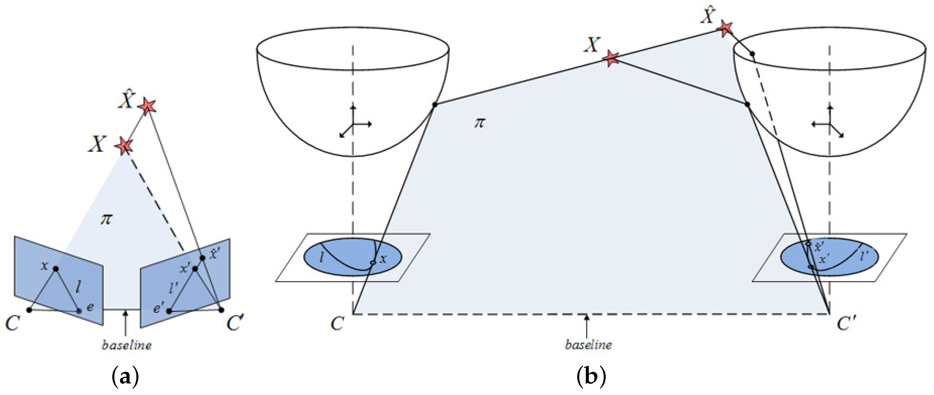
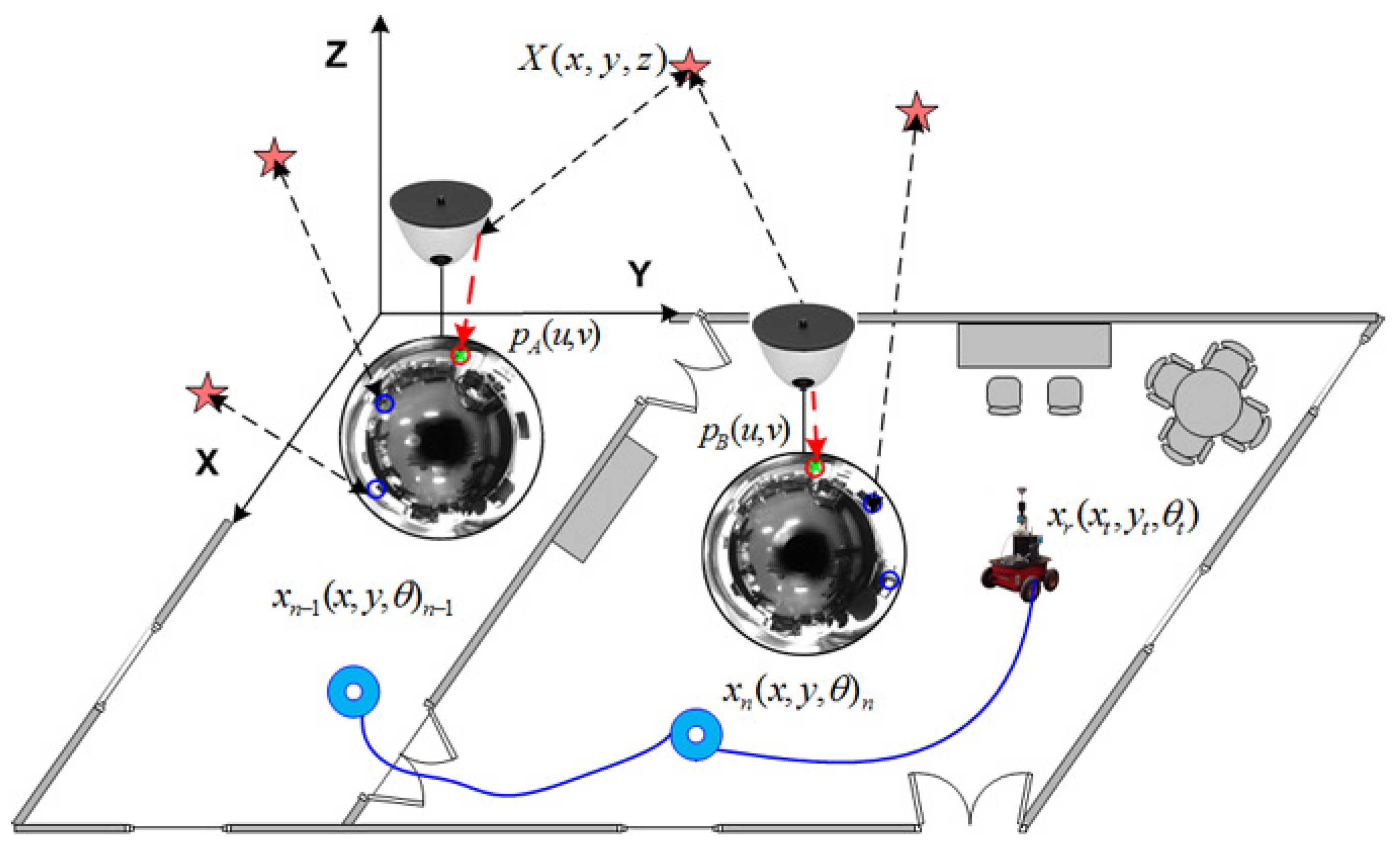
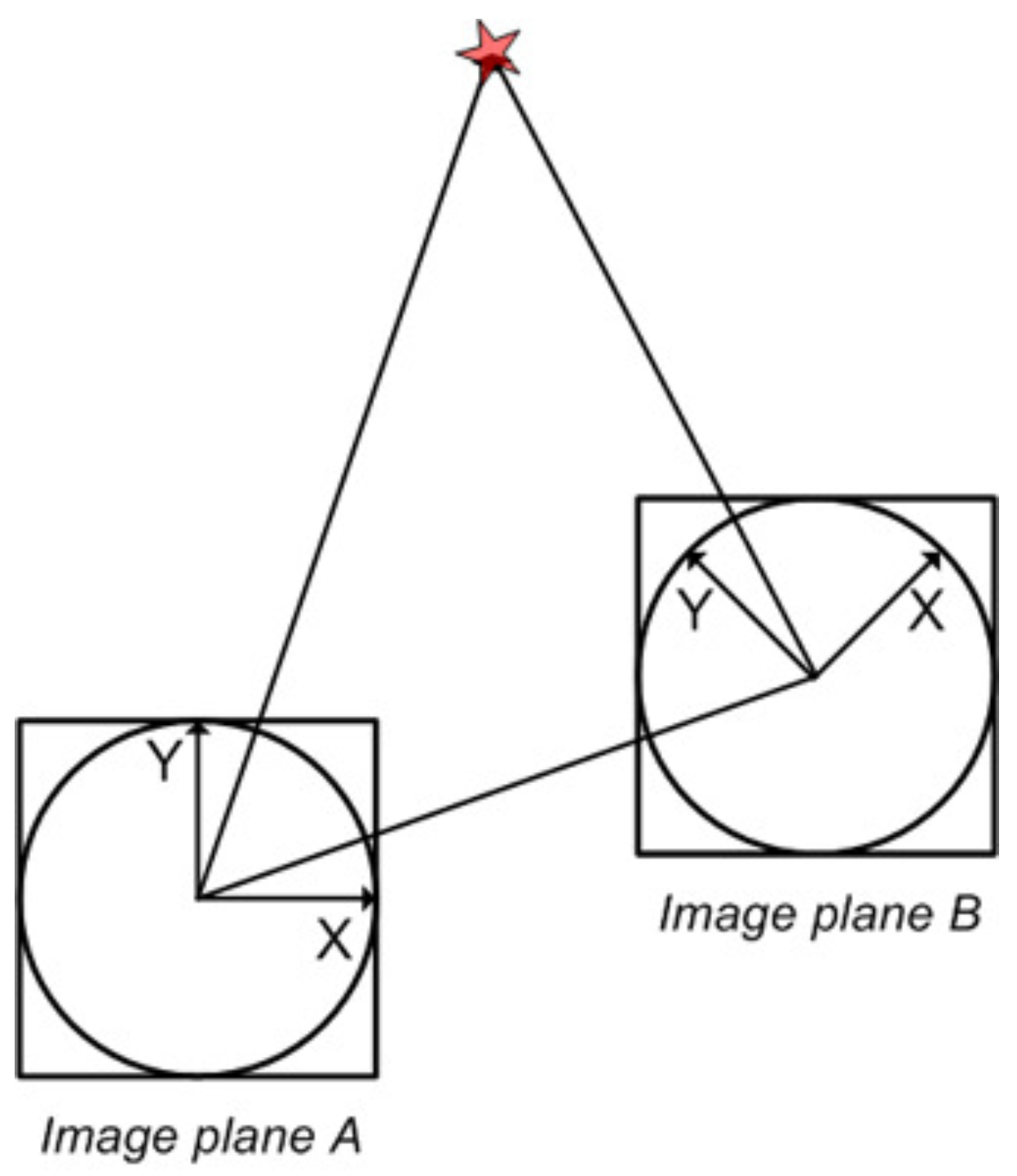
2.1. Epipolar Geometry
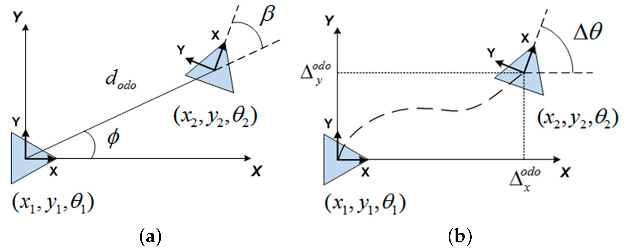
2.2. Motion Recovery
2.3. Adaptive Matching
- Prediction
- Innovation
- Updatewhere the following terms are involved:
- : relation between the control input and the current state.
- : control input as the initial seed for the prediction.
- : relation between the observation and the current state.
- : jacobian of evaluated at the corresponding state.
- : jacobian of evaluated at the corresponding state.
- : covariance of the current uncertainty of the state.
- : covariance of the gaussian noise generated by the camera sensor.
- : covariance of the gaussian noise generated by the internal odometers.
- : gain matrix of the filter which plays the role of weighting.
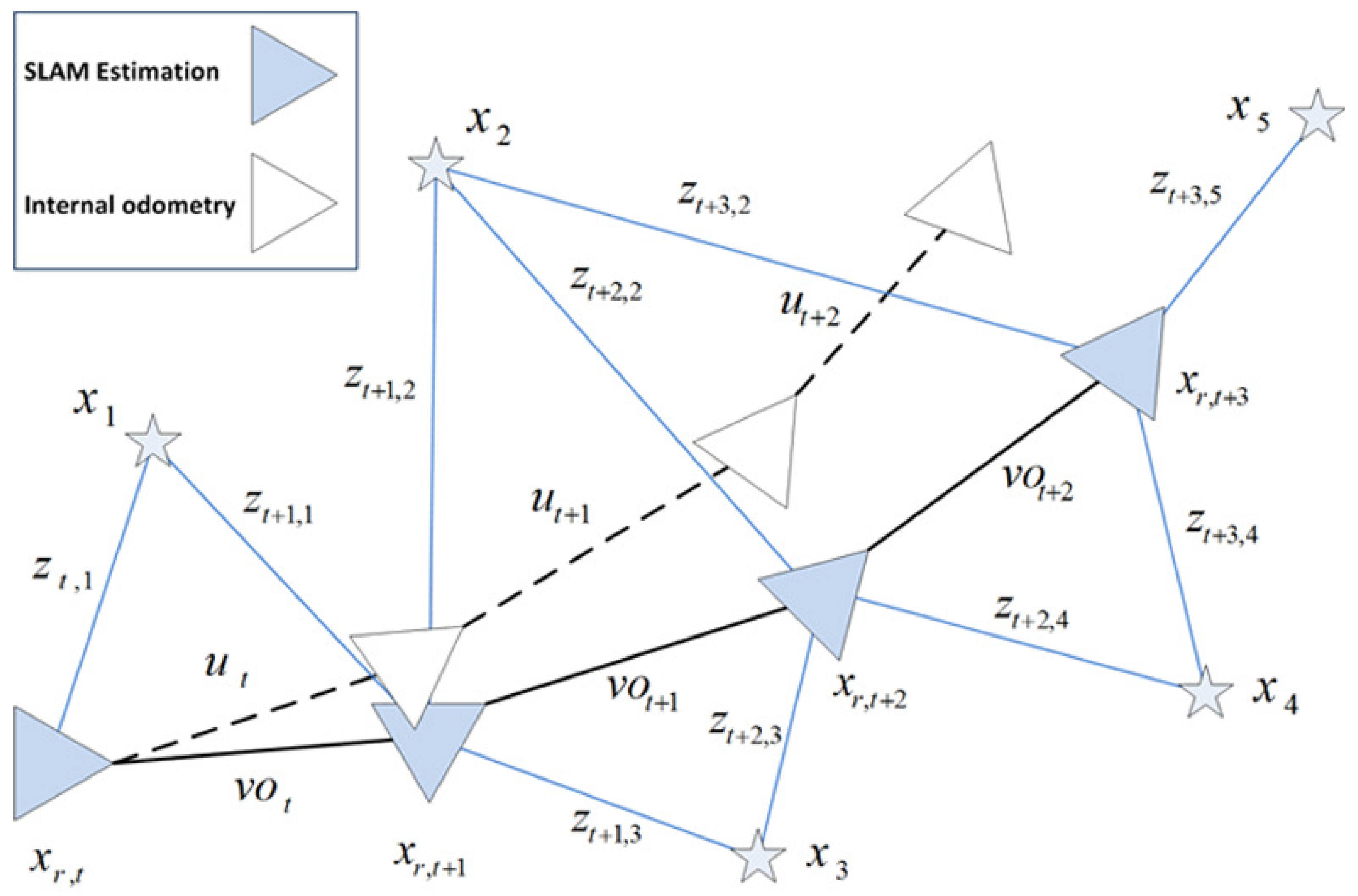
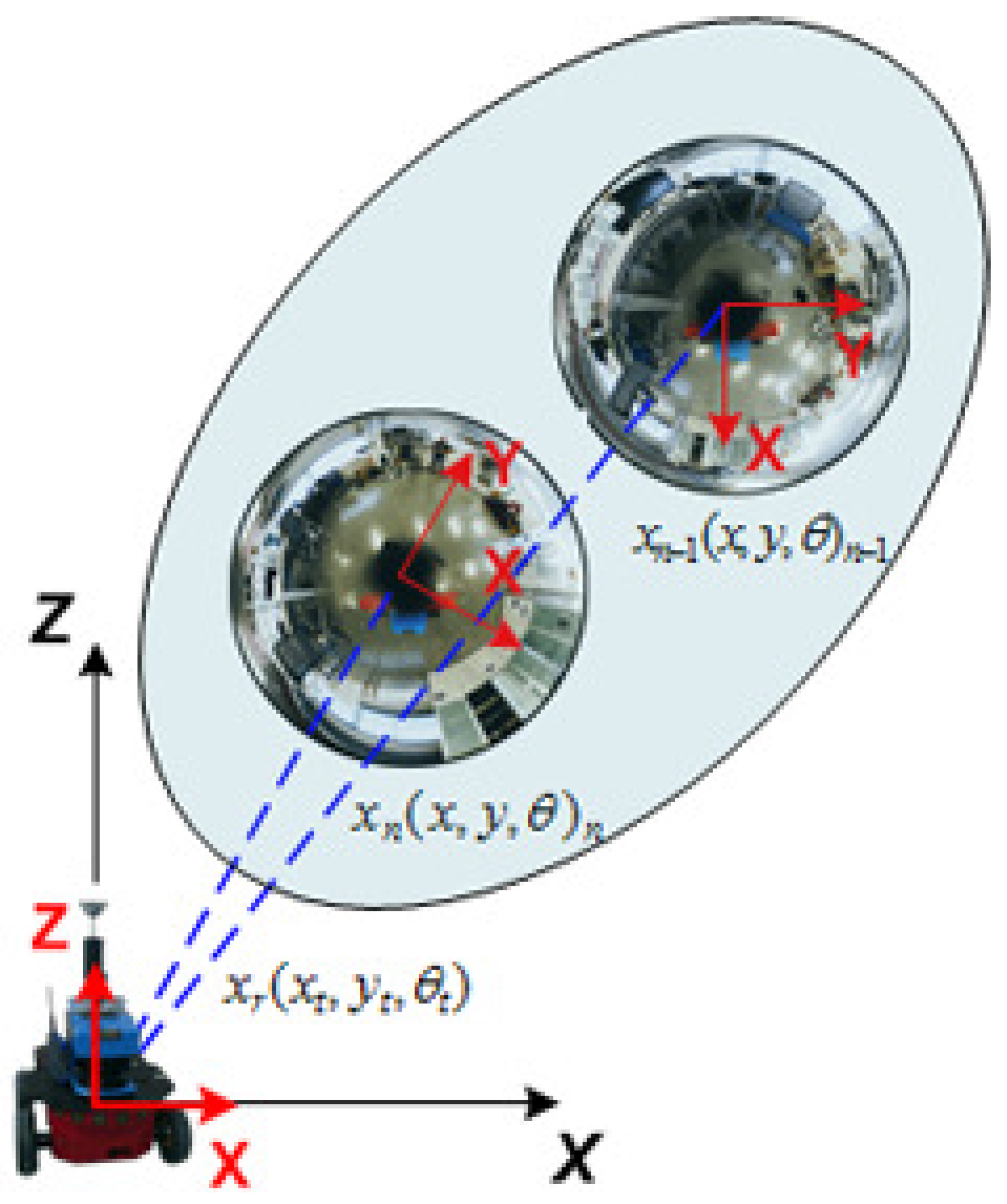
3. View-Based SLAM
- (i) initialization of views in the map.
- () observation model measurement.
- () data association.
3.1. View Initialization
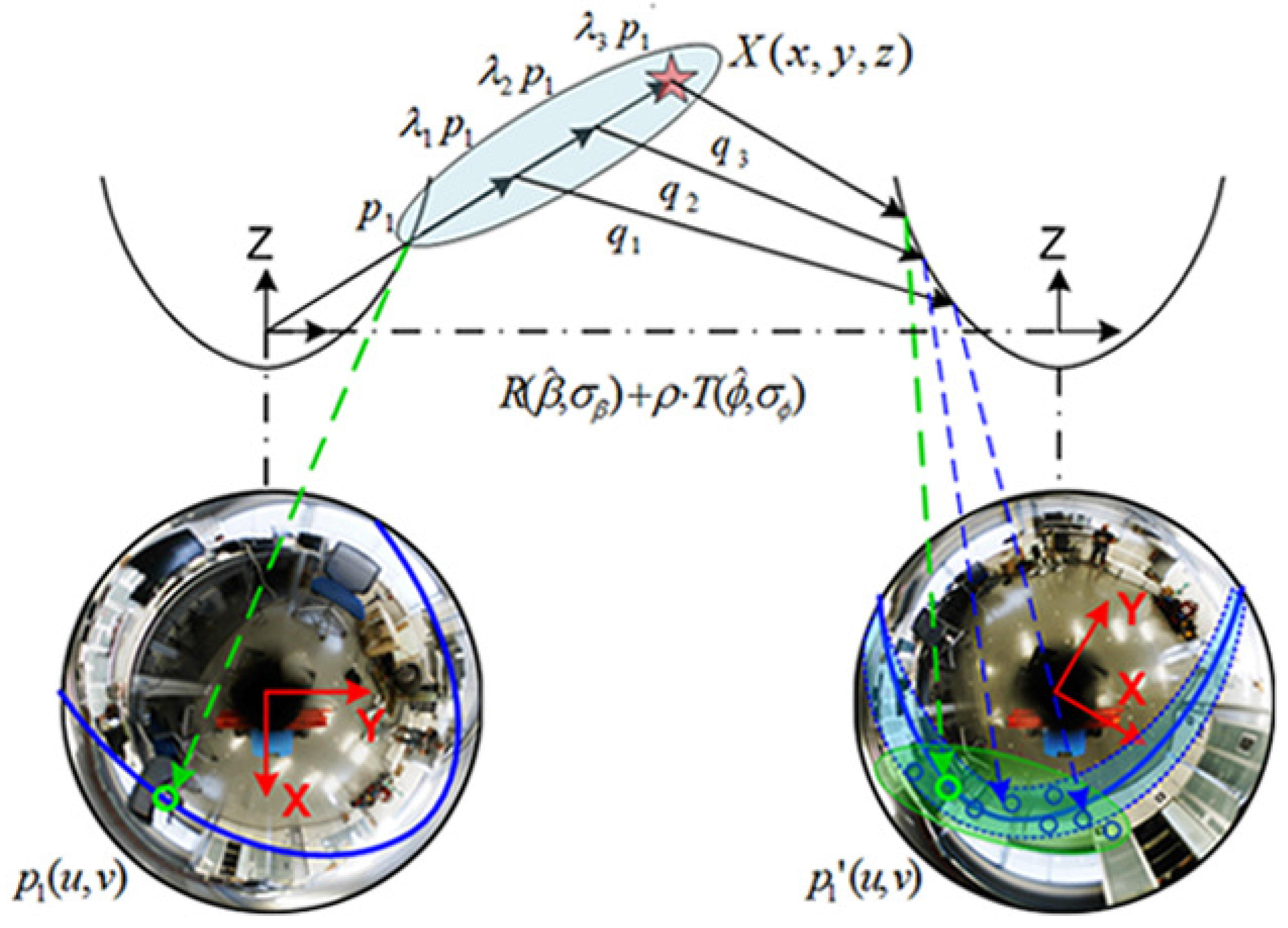
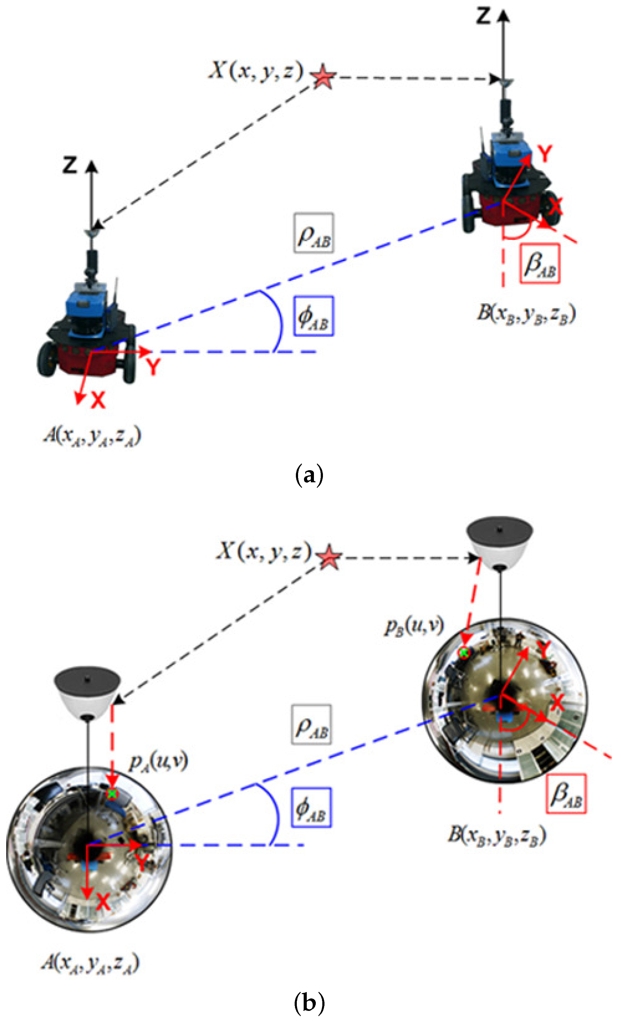
3.2. Observation Model
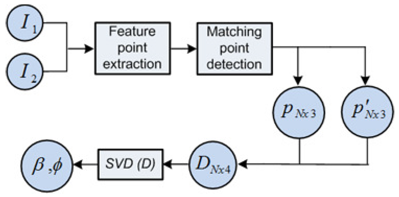
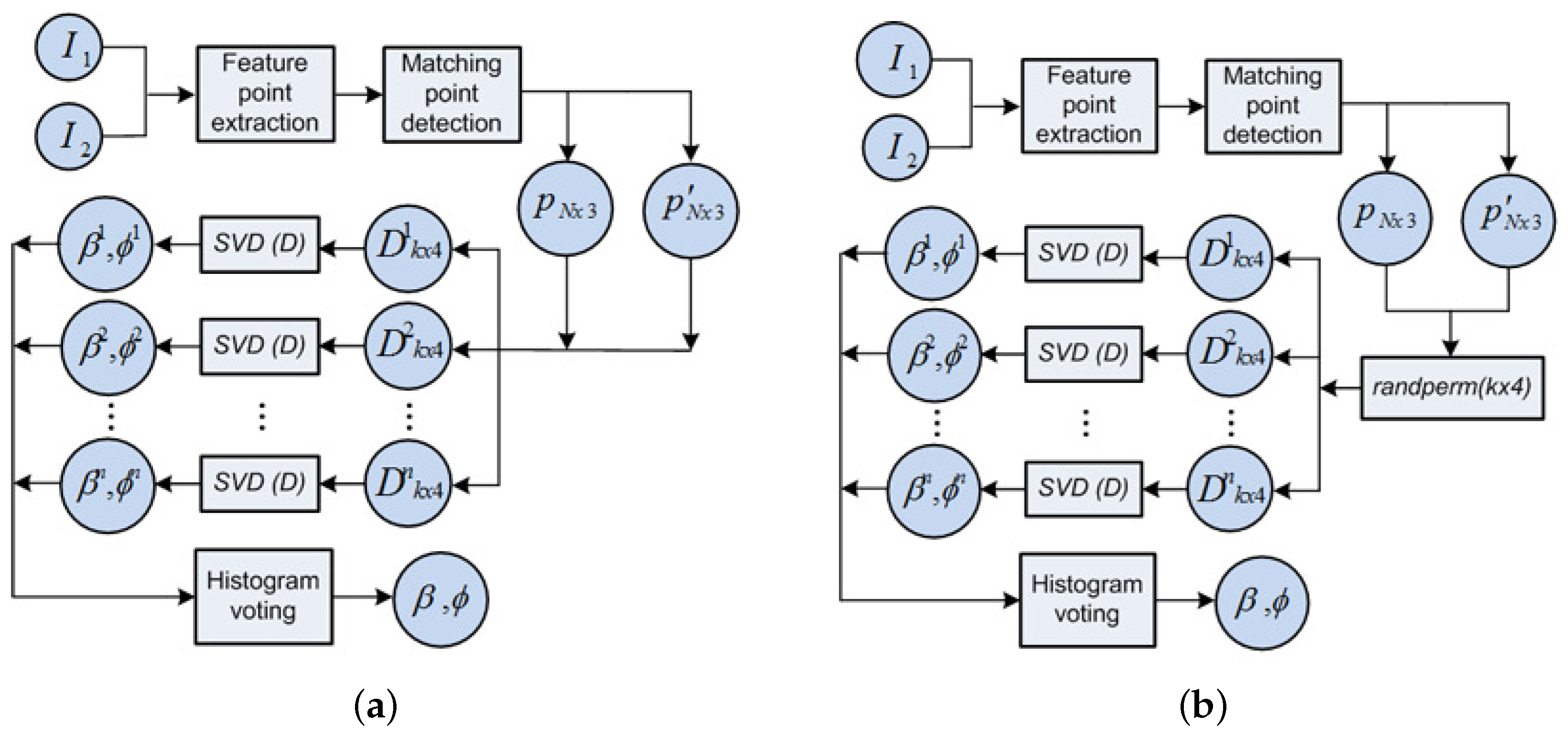
- (i) feature points, p and are extracted from the omnidirectional images and .
- () the total N points input the SVD solver at once, as , namely in Equation (7).
- () ultimately, they produce the single solution, as the observation measurement (β,).
3.3. Data Association
| Algorithm 1 Data Association |
| Require: Inputs ∈ ∀ n, where =[, , , … ] : Set of candidate views within range. : Views maximizing similarity ratio A. : Maximum range. : feature points on robot’s image at . : feature points on view . for i=1:N do if < then New candidate to the subset: =[, , …, ] end if end for for j=1:length() do Extracting on ∈ if =k then =[] end if end for return |
4. Results
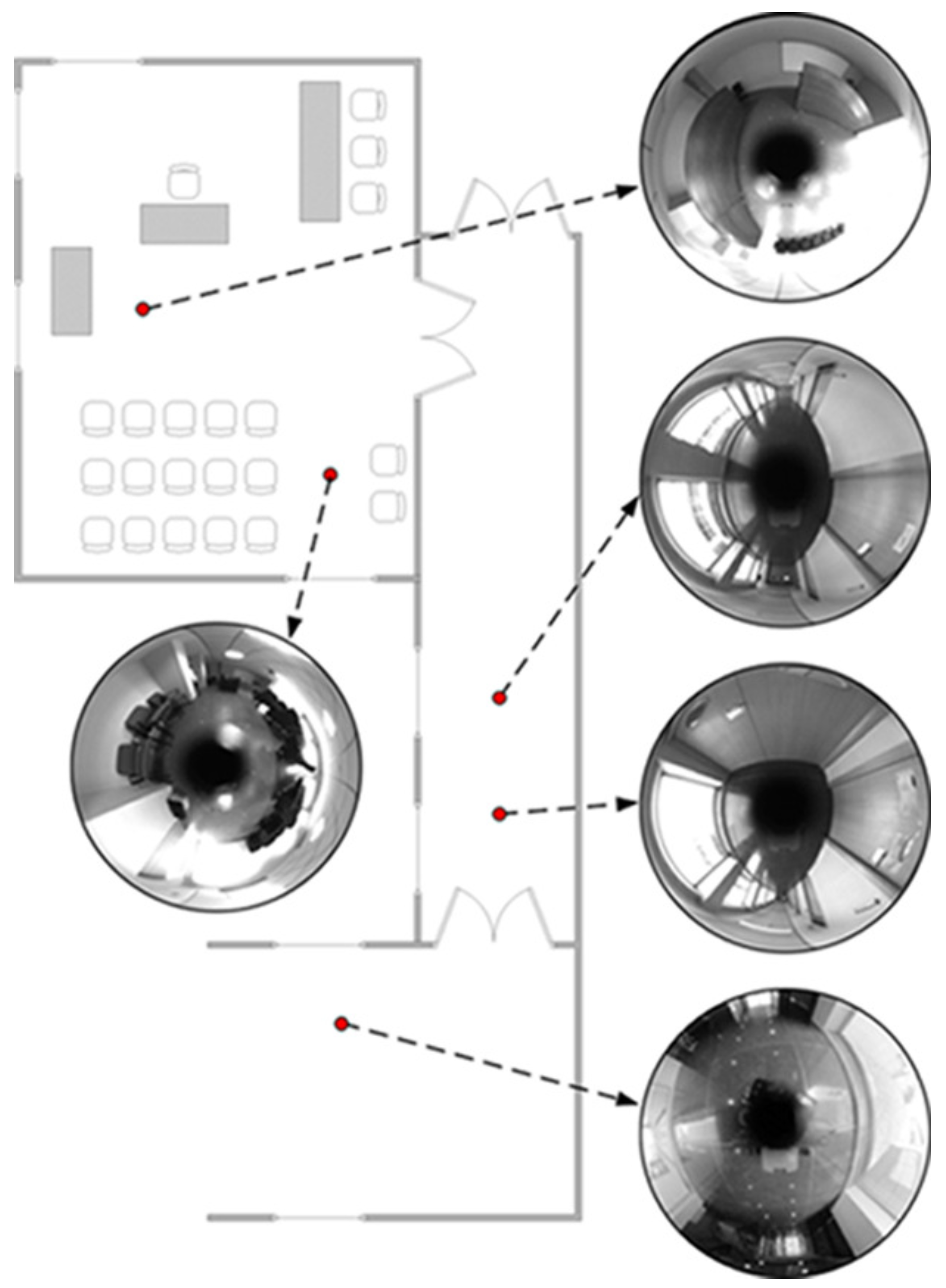
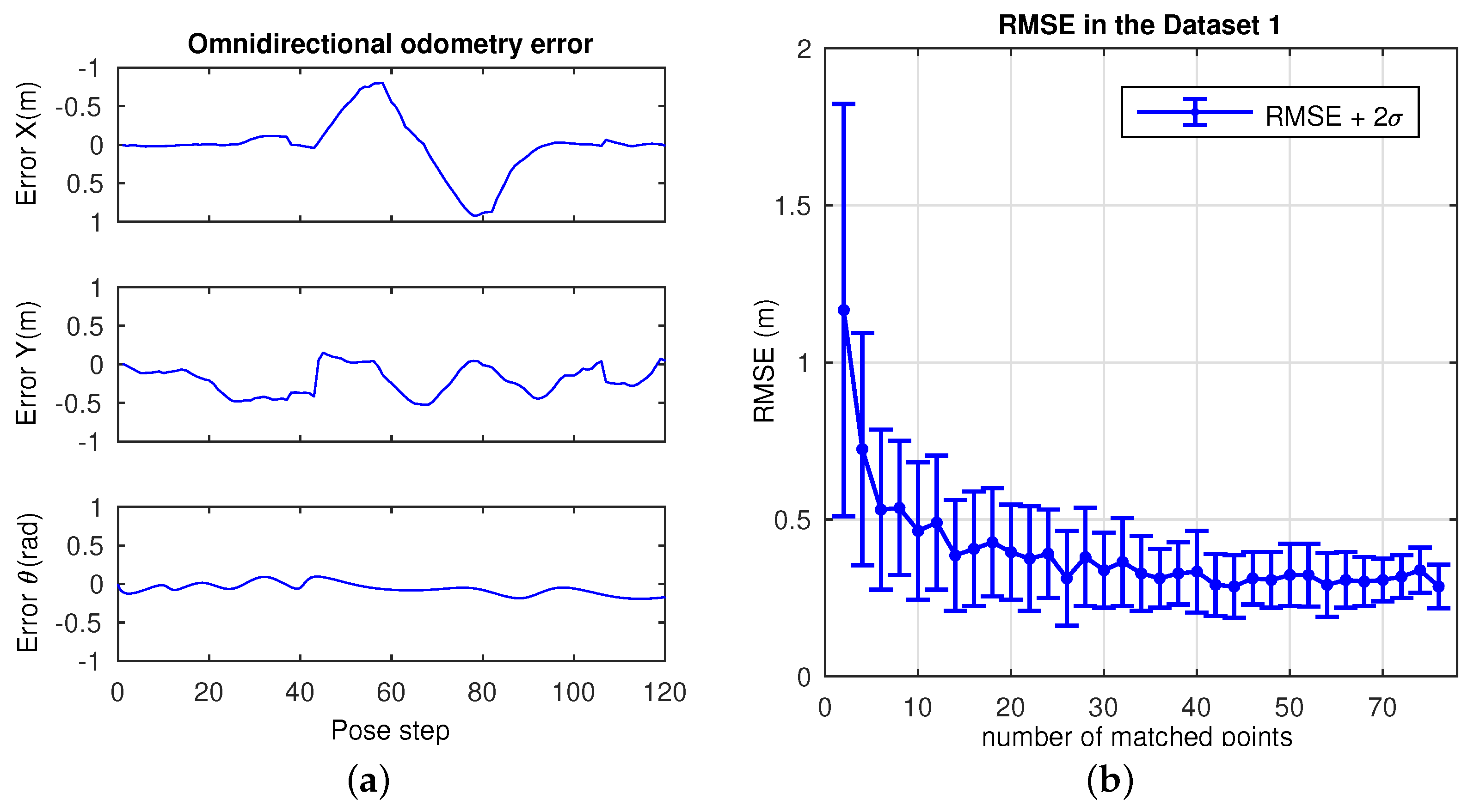
4.1. Omndirectional Odometry
Dataset 1
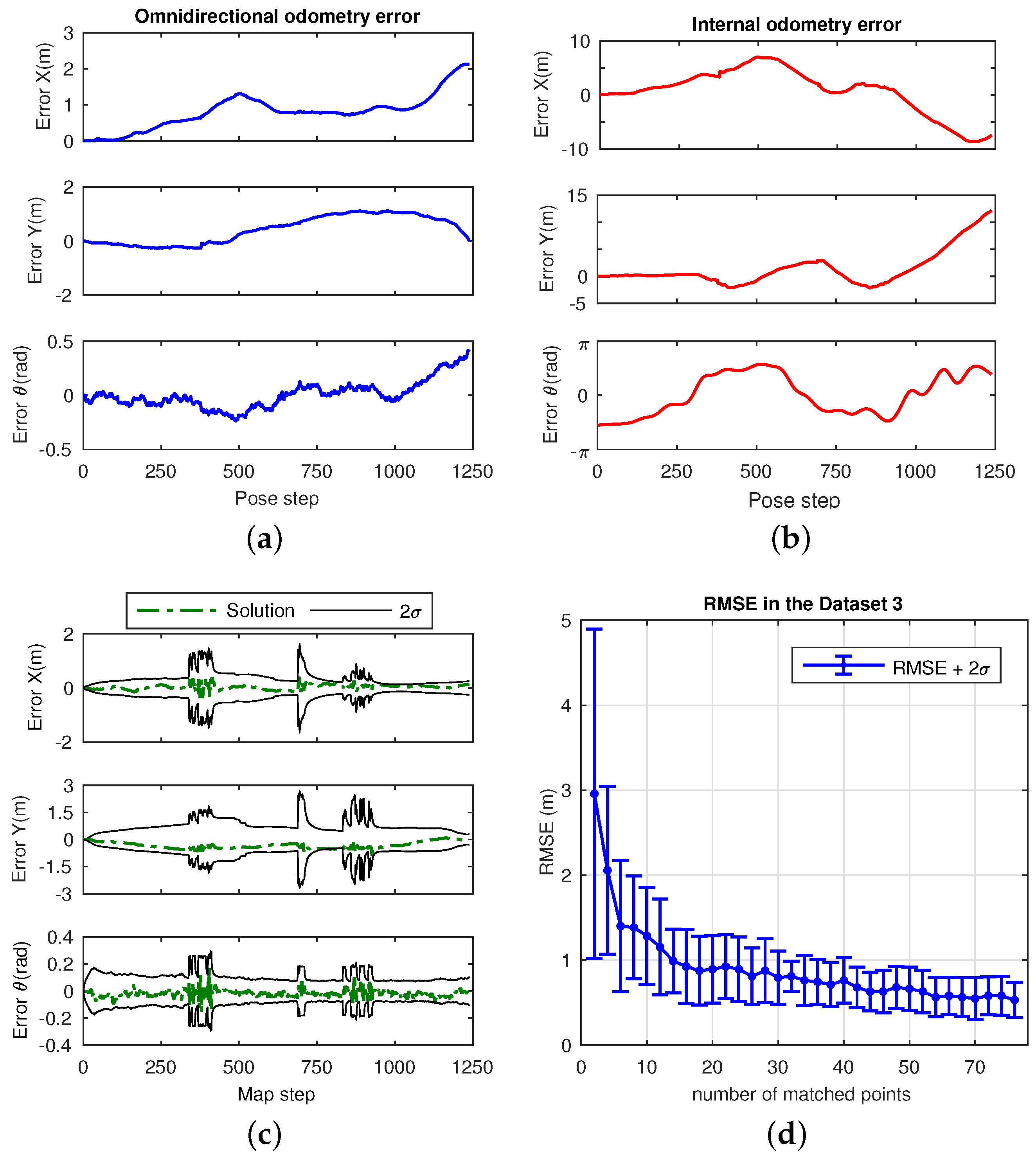
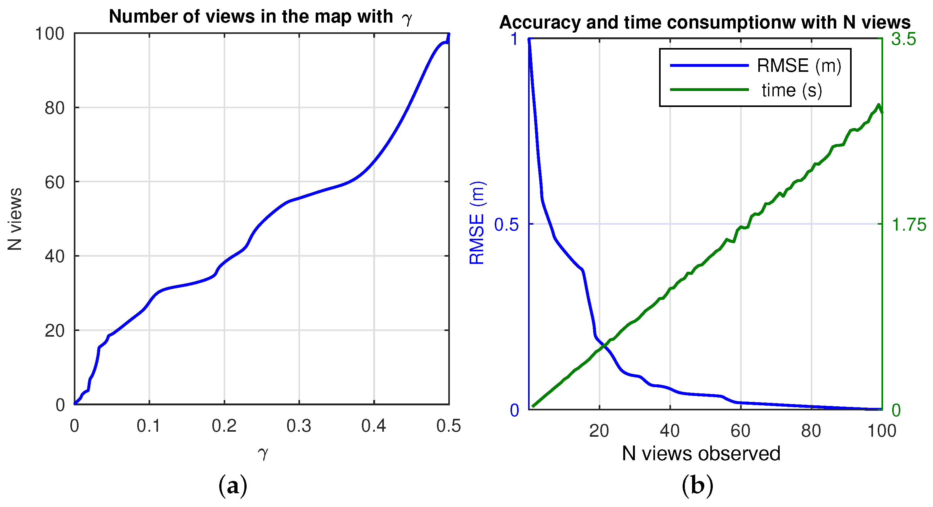
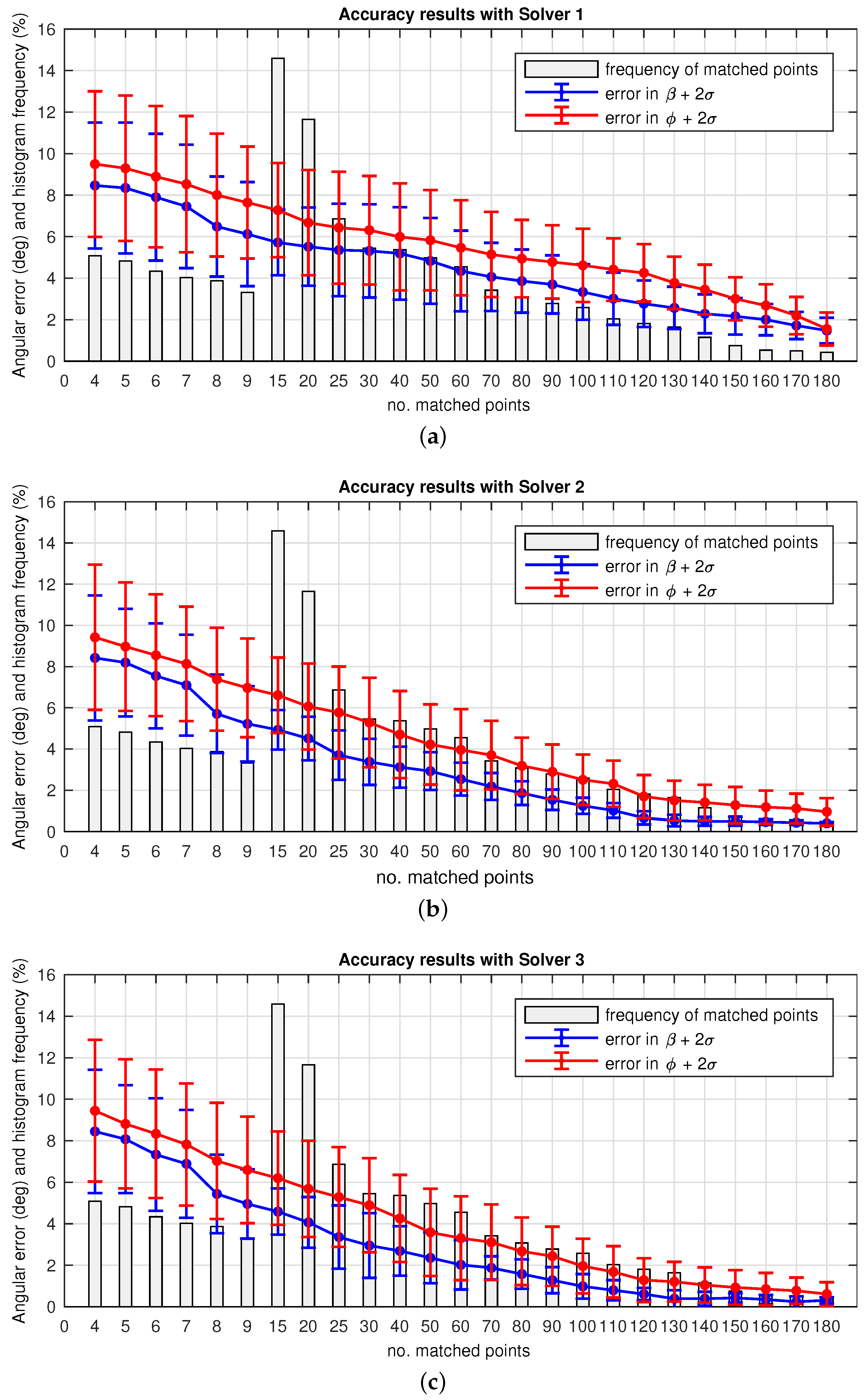
4.2. Performance: Accuracy
4.2.1. Solver 1
4.2.2. Solver 2
4.2.3. Solver 3
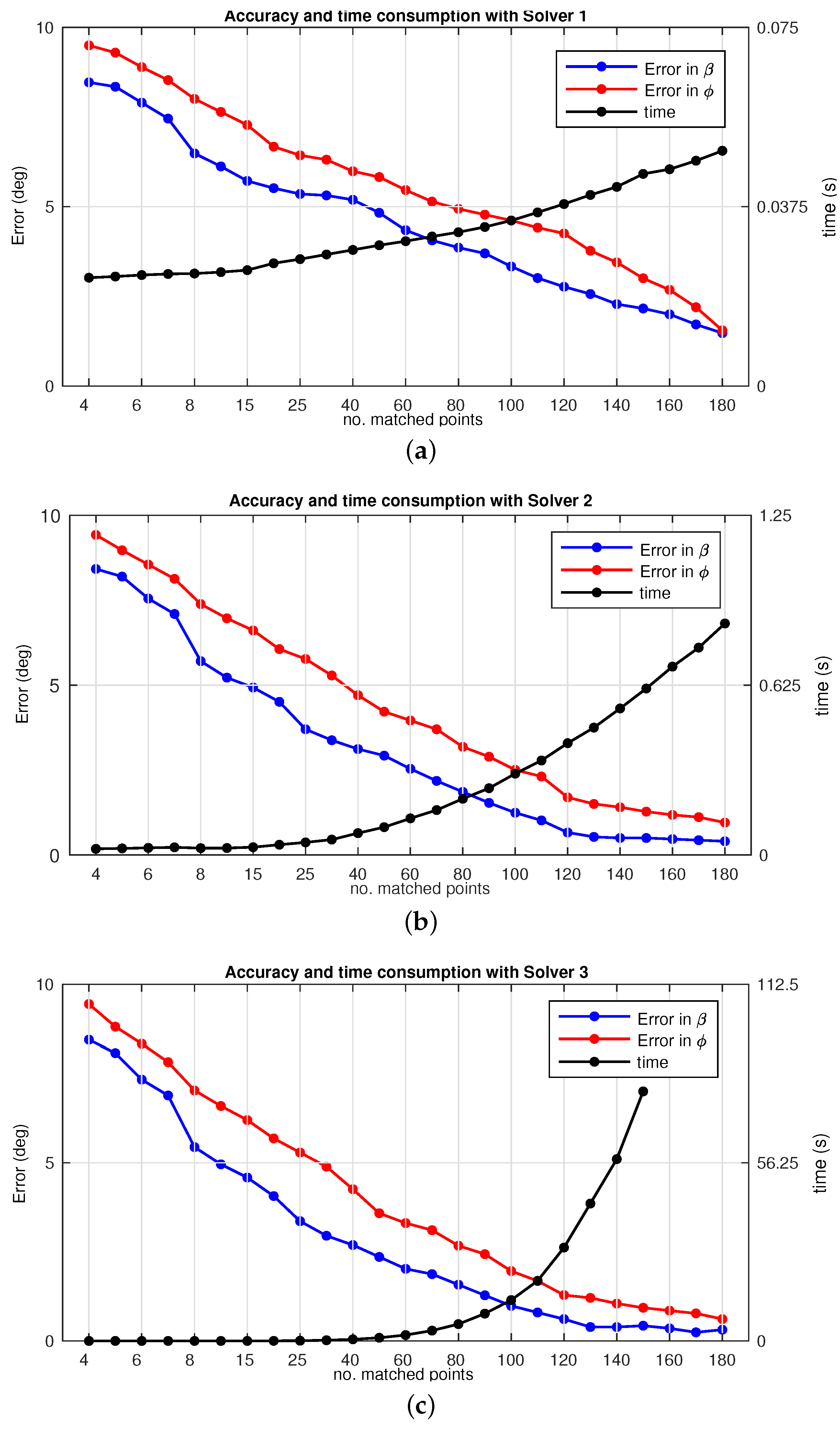
4.3. Performance: Time Consumption
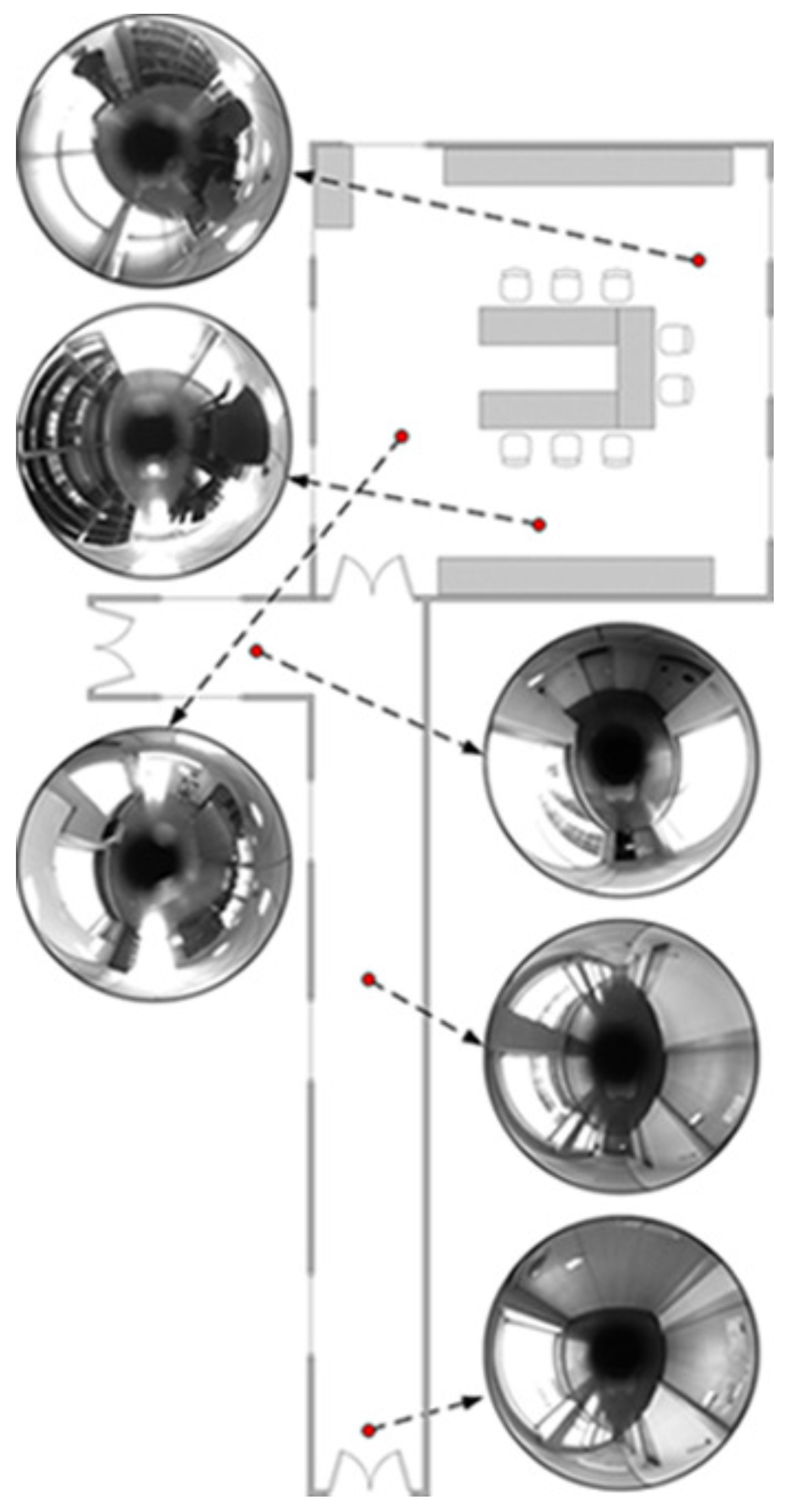
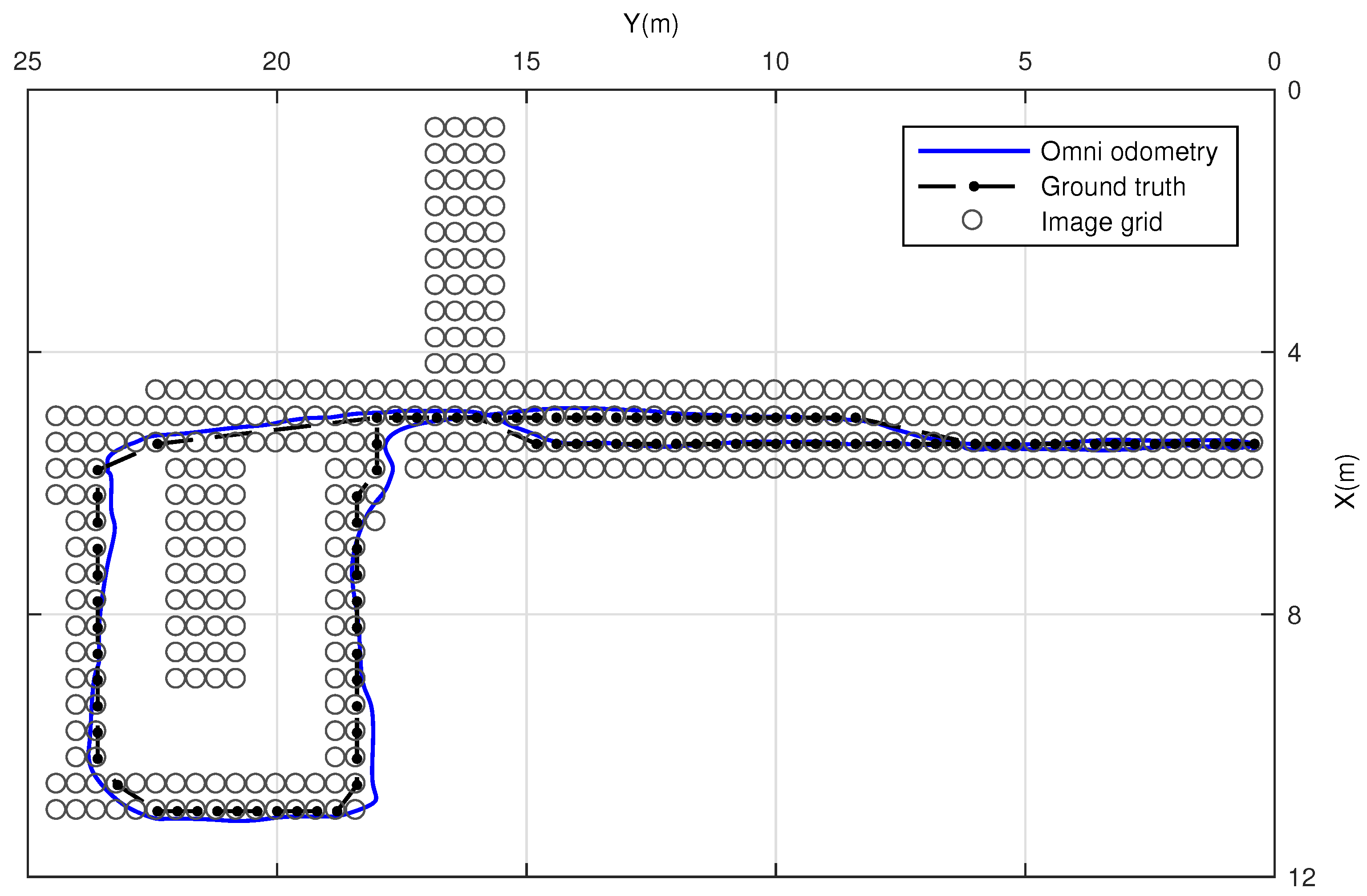
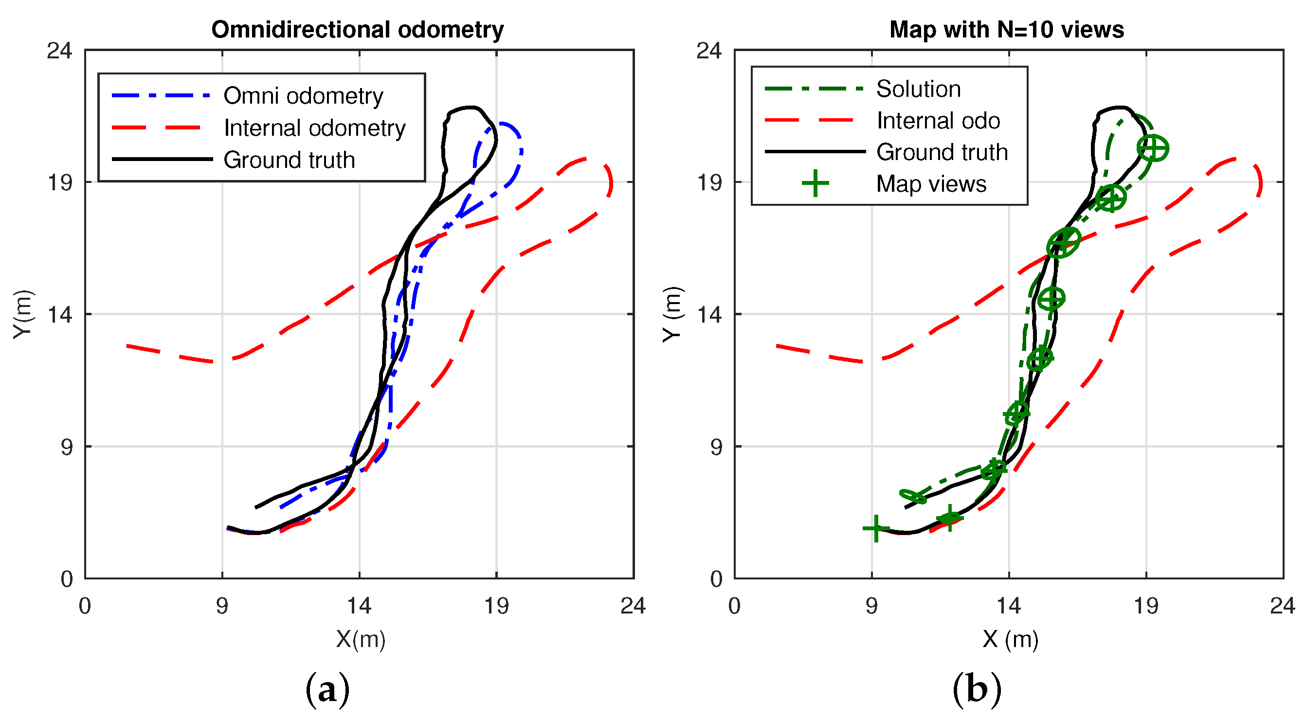
4.4. SLAM Results
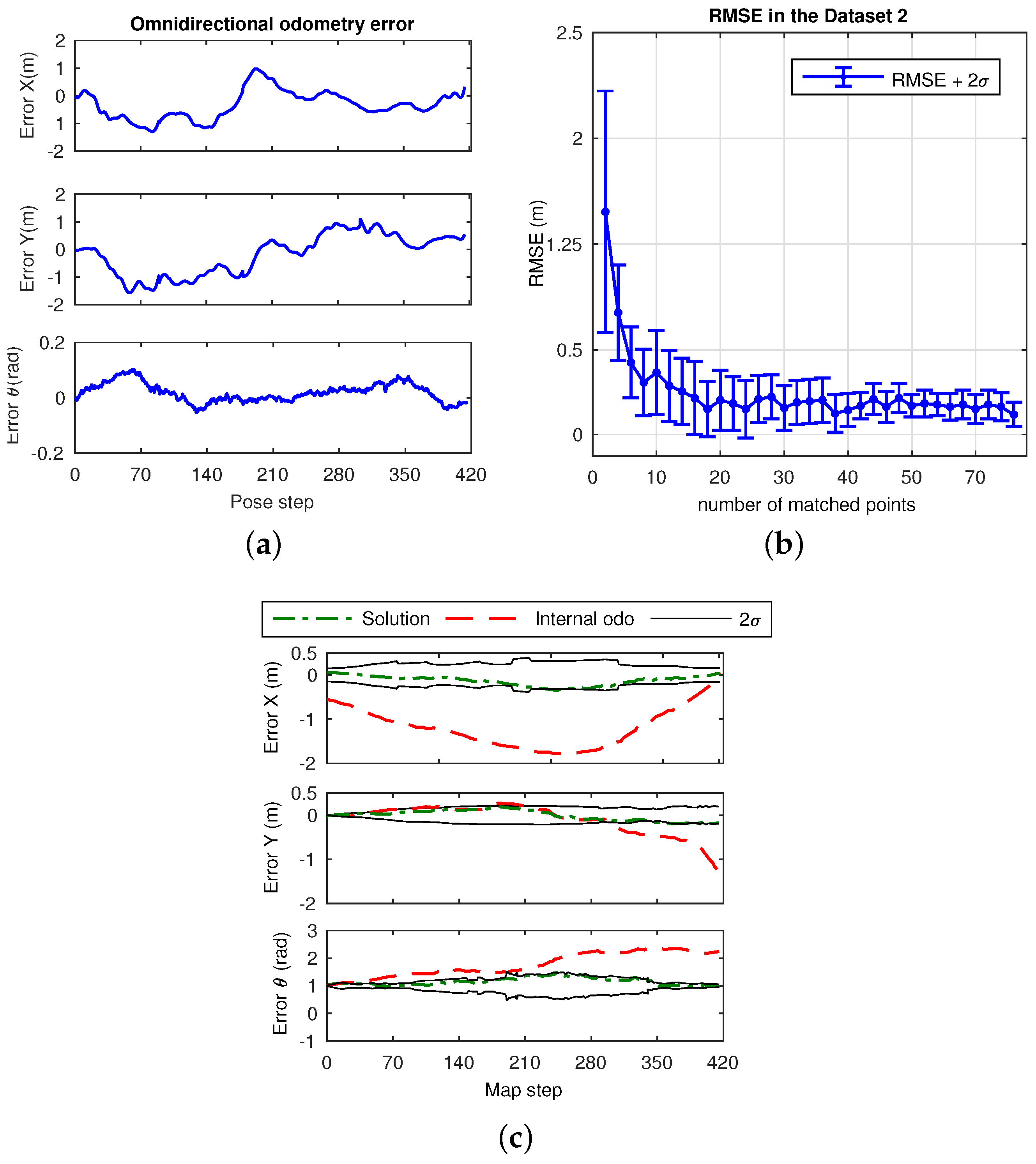
4.4.1. Dataset 2
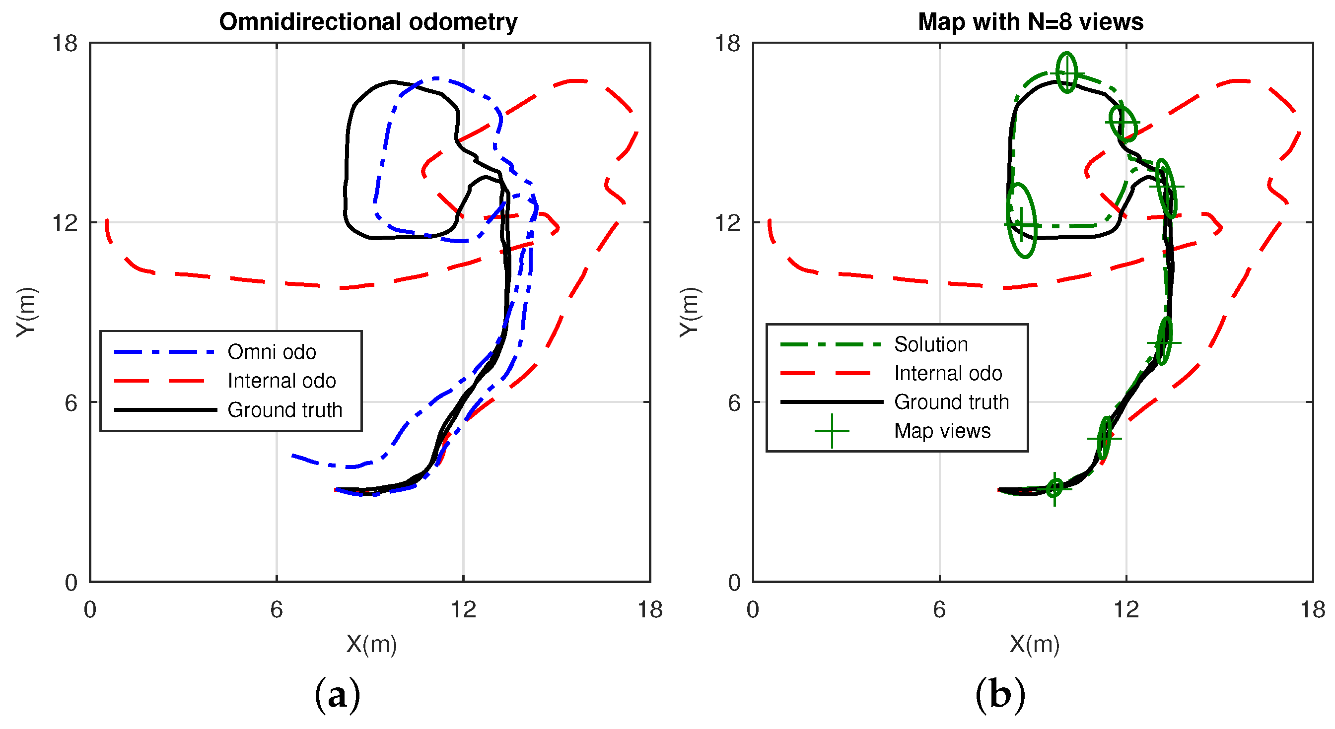
4.4.2. Dataset 3
5. Discussion
- (i) Better results are obtained at any solver case with higher number of matched points considered in order to compute the motion recovery. This implies a considerable increase on the computation time, which may become inviable.
- () Particularly, Solver 2 and Solver 3 are liable to require such time efforts, as observed in Figure 17. Despite this fact they provide useful outcomes in order to mitigate false positives.
- () Overall, a well devised tradeoff solution may be reached, depending on the final application. Solver 1 may provide sufficient accuracy at a low time consumption, for time demanding applications. The other two solver proposals can be advantageous under cases where the real need is to avoid false imparity, regardless the time consumed.
6. Conclusions
Acknowledgments
Author Contributions
Conflicts of Interest
Abbreviations
| SLAM | Simultaneous Localization and Mapping |
| EKF | Extended Kalman Filter |
| SVD | Single Value Decomposition |
| RMSE | Root Mean Squar Error |
References
- Borenstein, J.; Feng, L. Measurement and correction of systematic odometry errors in mobile robots. IEEE Trans. Robot. Autom. 1996, 12, 869–880. [Google Scholar] [CrossRef]
- Fox, D.; Burgard, W.; Thrun, S. Markov Localization for Mobile Robots in Dynamic Environments. J. Artif. Intell. Res. 1999, 11, 391–427. [Google Scholar]
- Martinelli, A. A possible strategy to evaluate the odometry error of a mobile robot. In Proceedings of the IEEE/RSJ International Conference on Intelligent Robots and Systems, Maui, HI, USA, 29 October–3 November 2001; Volume 4, pp. 1946–1951.
- Martinelli, A. The odometry error of a mobile robot with a synchronous drive system. IEEE Trans. Robot. Autom. 2002, 18, 399–405. [Google Scholar] [CrossRef]
- Krivi, S.; Mrzi, A.; Velagi, J.; Osmi, N. Optimization based algorithm for correction of systematic odometry errors of mobile robot. In Proceedings of the 9th Asian Control Conference (ASCC), Istanbul, Turkey, 23–26 June 2013; pp. 1–6.
- Xu, H.; Collins, J.J. Estimating the Odometry Error of a Mobile Robot by Neural Networks. In Proceedings of the International Conference on Machine Learning and Applications (ICMLA), Miami Beach, FL, USA, 13–15 December 2009; pp. 378–385.
- Yu, J.; Park, S.S.; Hyun, W.K.; Choi, H.Y. A correction system of odometry error for simultaneous map building based on sensor fusion. In Proceedings of the International Conference on Smart Manufacturing Application (ICSMA), Goyang-si, Korea, 9–11 April 2008; pp. 393–396.
- Ndjeng, A.N.; Gruyer, D.; Glaser, S.; Lambert, A. Low cost IMU-Odometer-GPS ego localization for unusual maneuvers. Inf. Fusion 2011, 12, 264–274. [Google Scholar] [CrossRef]
- Agrawal, M.; Konolige, K. Real-time Localization in Outdoor Environments using Stereo Vision and Inexpensive GPS. In Proceedings of the International Conference on Pattern Recognition (ICPR), Hong Kong, China, 20–24 August 2006; pp. 1063–1068.
- Golban, C.; Cobarzan, P.; Nedevschi, S. Direct formulas for stereo-based visual odometry error modeling. In Proceedings of the IEEE International Conference on Intelligent Computer Communication and Processing (ICCP), Cluj-Napoca, Romania, 3–5 September 2015; pp. 197–202.
- Nister, D.; Naroditsky, O.; Bergen, J. Visual odometry. In Proceedings of the IEEE International Conference on Computer Vision and Pattern Recognition (CVPR), Washington, DC, USA, 27 June–2 July 2004; Volume 1, pp. 652–659.
- Usenko, V.; Engel, J.; Stuckler, J.; Cremers, D. Direct visual-inertial odometry with stereo cameras. In Proceedings of the IEEE International Conference on Robotics and Automation (ICRA), Stockholm, Sweden, 16–21 May 2016; pp. 1885–1892.
- Engel, J.; Cremers, D. Scale-aware navigation of a lowcost quadrocopter with a monocular camera. Robot. Auton. Syst. 2014, 62, 1646–1656. [Google Scholar] [CrossRef]
- Nister, D. Preemptive RANSAC for live structure and motion estimation. Mach. Vis. Appl. 2005, 16, 321–329. [Google Scholar] [CrossRef]
- Nister, D.; Naroditsky, O.; Bergen, J. Visual odometry for ground vehicle applications. J. Field Robot. 2006, 23, 3–20. [Google Scholar] [CrossRef]
- Corke, P.; Strelow, D.; Singh, S. Omnidirectional visual odometry for a planetary rover. In Proceedings of the 2004 IEEE/RSJ International Conference on Intelligent Robots and Systems (IROS), Sendai, Japan, 28 September–2 October 2004; Volume 4, pp. 4007–4012.
- Scaramuzza, D.; Fraundorfer, F.; Siegwart, R. Real-Time Monocular Visual Odometry for On-Road Vehicles with 1-Point RANSAC. In Proceedings of the IEEE International Conference on Robotics & Automation (ICRA), Kobe, Japan, 12–17 May 2009; pp. 4293–4299.
- Tardif, J.P.; Pavlidis, Y.; Daniilidis, K. Monocular visual odometry in urban environments using an omnidirectional camera. In Proceedings of the IEEE/RSJ International Conference on Intelligent Robots and Systems (IROS), Nice, France, 22–26 September 2008; pp. 2531–2538.
- Scaramuzza, D.; Siegwart, R. Appearance-Guided Monocular Omnidirectional Visual Odometry for Outdoor Ground Vehicles. IEEE Trans. Robot. 2008, 24, 1015–1026. [Google Scholar] [CrossRef]
- Valiente, D.; Fernández, L.; Gil, A.; Payá, L.; Reinoso, Ó. Visual Odometry through Appearance- and Feature-Based Method with Omnidirectional Images. J. Robot. 2012, 2012, 797063. [Google Scholar] [CrossRef]
- Se, S.; Lowe, D.; Little, J. Vision-based Mobile Robot Localization and Mapping using Scale-Invariant Features. In Proceedings of the IEEE International Conference on Robotics and Automation (ICRA), Seoul, Korea, 21–26 May 2001; Volume 2, pp. 2051–2058.
- Chli, M.; Davison, A.J. Active Matching for Visual Tracking. Robot. Auton. Syst. 2009, 57, 1173–1187. [Google Scholar] [CrossRef]
- Zhou, D.; Fremont, V.; Quost, B.; Wang, B. On Modeling Ego-Motion Uncertainty for Moving Object Detection from a Mobile Platform. In Proceedings of the IEEE Intelligent Vehicles Symposium, Dearborn, MI, USA, 8–11 June 2014; pp. 1332–1338.
- Lundquist, C.; Schön, T.B. Joint ego-motion and road geometry estimation. Inf. Fusion 2011, 12, 253–263. [Google Scholar] [CrossRef]
- Liu, Y.; Xiong, R.; Wang, Y.; Huang, H.; Xie, X.; Liu, X.; Zhang, G. Stereo Visual-Inertial Odometry With Multiple Kalman Filters Ensemble. IEEE Trans. Ind. Electron. 2016, 63, 6205–6216. [Google Scholar] [CrossRef]
- Whelan, T.; Johannsson, H.; Kaess, M.; Leonard, J.J.; McDonald, J. Robust real-time visual odometry for dense RGB-D mapping. In Proceedings of the IEEE International Conference on Robotics and Automation, Karlsruhe, Germany, 6–10 May 2013; pp. 5724–5731.
- Jiang, Y.; Xu, Y.; Liu, Y. Performance evaluation of feature detection and matching in stereo visual odometry. Neurocomputing 2013, 120, 380–390. [Google Scholar] [CrossRef]
- Suaib, N.M.; Marhaban, M.H.; Saripan, M.I.; Ahmad, S.A. Performance evaluation of feature detection and feature matching for stereo visual odometry using SIFT and SURF. In Proceedings of the IEEE Regin 10 Symposium, Kuala Lumpur, Malaysia, 14–16 April 2014; pp. 200–203.
- Engel, J.; Schöps, T.; Cremers, D. LSD-SLAM: Large-Scale Direct Monocular SLAM. In European Conference on Computer Vision (ECCV); Springer: Zurich, Switzerland, 2014; pp. 834–849. [Google Scholar]
- Engel, J.; Stuckler, J.; Cremers, D. Large-scale direct SLAM with stereo cameras. In Proceedings of the IEEE/RSJ International Conference on Intelligent Robots and Systems (IROS), Hamburg, Germany, 28 September–2 October 2015; pp. 1935–1942.
- Caruso, D.; Engel, J.; Cremers, D. Large-scale direct SLAM for omnidirectional cameras. In Proceedings of the IEEE/RSJ International Conference on Intelligent Robots and Systems (IROS), Hamburg, Germany, 28 September–2 October 2015; pp. 141–148.
- Goel, P.; Roumeliotis, S.I.; Sukhatme, G.S. Robust localization using relative and absolute position estimates. In Proceedings of the 1999 IEEE/RSJ International Conference on Intelligent Robots and Systems. Human and Environment Friendly Robots with High Intelligence and Emotional Quotients (Cat. No.99CH36289), Kyongju, Korea, 17–21 October 1999; Volume 2, pp. 1134–1140.
- Wang, T.; Wu, Y.; Liang, J.; Han, C.; Chen, J.; Zhao, Q. Analysis and Experimental Kinematics of a Skid-Steering Wheeled Robot Based on a Laser Scanner Sensor. Sensors 2015, 15, 9681–9702. [Google Scholar] [CrossRef] [PubMed]
- Scaramuzza, D.; Martinelli, A.; Siegwart, R. A Toolbox for Easily Calibrating Omnidirectional Cameras. In Proceedings of the IEEE/RSJ International Conference on Intelligent Robots and Systems (IROS), Beijing, China, 9–15 October 2006; pp. 5695–5701.
- Hartley, R.; Zisserman, A. Multiple View Geometry in Computer Vision; Cambridge University Press: Cambridge, UK, 2004. [Google Scholar]
- Longuet-Higgins, H.C. A computer algorithm for reconstructing a scene from two projections. Nature 1985, 293, 133–135. [Google Scholar] [CrossRef]
- Servos, J.; Smart, M.; Waslander, S. Underwater stereo SLAM with refraction correction. In Proceedings of the IEEE/RSJ International Conference on Intelligent Robots and Systems (IROS), Tokyo, Japan, 3–7 November 2013; pp. 3350–3355.
- Bay, H.; Tuytelaars, T.; Van Gool, L. Speeded Up Robust Features (SURF). Comput. Vis. Image Underst. 2008, 110, 346–359. [Google Scholar] [CrossRef]
- Gil, A.; Reinoso, O.; Ballesta, M.; Juliá, M.; Payá, L. Estimation of Visual Maps with a Robot Network Equipped with Vision Sensors. Sensors 2010, 10, 5209–5232. [Google Scholar] [CrossRef] [PubMed]
- Davison, A.J. Real-Time Simultaneous Localisation and Mapping with a Single Camera. In Proceedings of the International Conference on Computer Vision, Washington, DC, USA, 13–16 October 2003; Volume 2, pp. 1403–1410.
- Payá, L.; Amorós, F.; Fernández, L.; Reinoso, O. Performance of Global-Appearance Descriptors in Map Building and Localization Using Omnidirectional Vision. Sensors 2014, 14, 3033–3064. [Google Scholar] [CrossRef] [PubMed]
- Neira, J.; Tardós, J.D. Data association in stochastic mapping using the joint compatibility test. IEEE Trans. Robot. Autom. 2001, 17, 890–897. [Google Scholar] [CrossRef]
- Li, Y.; Li, S.; Song, Q.; Liu, H.; Meng, M.H. Fast and Robust Data Association Using Posterior Based Approximate Joint Compatibility Test. IEEE Trans. Ind. Inf. 2014, 10, 331–339. [Google Scholar] [CrossRef]
- Stachniss, C.; Grisetti, G.; Haehnel, D.; Burgard, W. Improved Rao-Blackwellized Mapping by Adaptive Sampling and Active Loop-Closure. In Proceedings of the Workshop on Self-Organization of Adaptive Behavior (SOAVE), Ilmenau, Germany, 28–30 September 2004; pp. 1–15.
- Grisetti, G.; Stachniss, C.; Burgard, W. Improved Techniques for Grid Mapping With Rao-Blackwellized Particle Filters. IEEE Trans. Robot. 2007, 23, 34–46. [Google Scholar] [CrossRef]


© 2017 by the authors. Licensee MDPI, Basel, Switzerland. This article is an open access article distributed under the terms and conditions of the Creative Commons Attribution (CC BY) license ( http://creativecommons.org/licenses/by/4.0/).
Share and Cite
Valiente, D.; Gil, A.; Reinoso, Ó.; Juliá, M.; Holloway, M. Improved Omnidirectional Odometry for a View-Based Mapping Approach. Sensors 2017, 17, 325. https://doi.org/10.3390/s17020325
Valiente D, Gil A, Reinoso Ó, Juliá M, Holloway M. Improved Omnidirectional Odometry for a View-Based Mapping Approach. Sensors. 2017; 17(2):325. https://doi.org/10.3390/s17020325
Chicago/Turabian StyleValiente, David, Arturo Gil, Óscar Reinoso, Miguel Juliá, and Mathew Holloway. 2017. "Improved Omnidirectional Odometry for a View-Based Mapping Approach" Sensors 17, no. 2: 325. https://doi.org/10.3390/s17020325
APA StyleValiente, D., Gil, A., Reinoso, Ó., Juliá, M., & Holloway, M. (2017). Improved Omnidirectional Odometry for a View-Based Mapping Approach. Sensors, 17(2), 325. https://doi.org/10.3390/s17020325