
A Novel General Imaging Formation Algorithm for GNSS-Based Bistatic SAR


Abstract
:1. Introduction
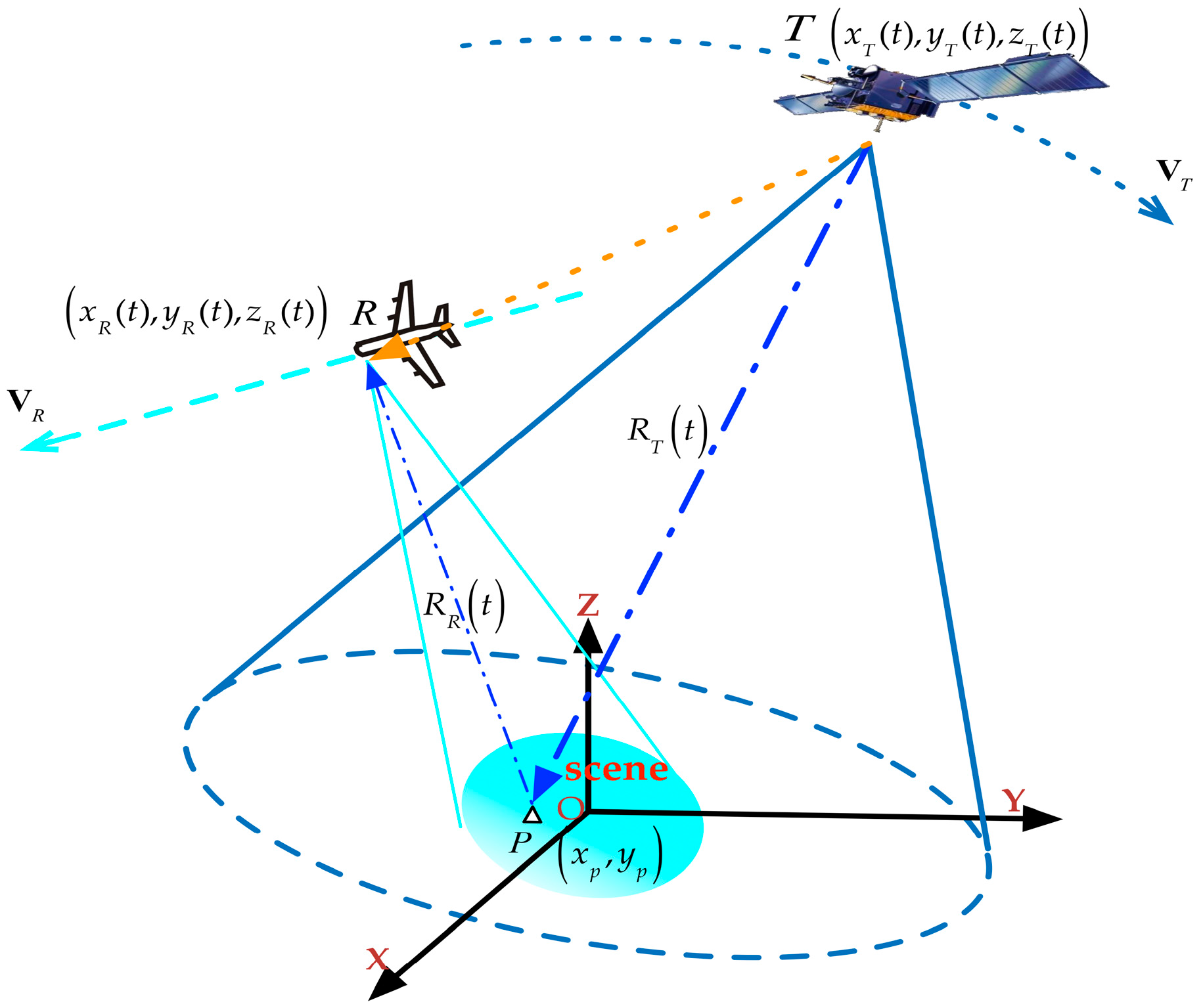
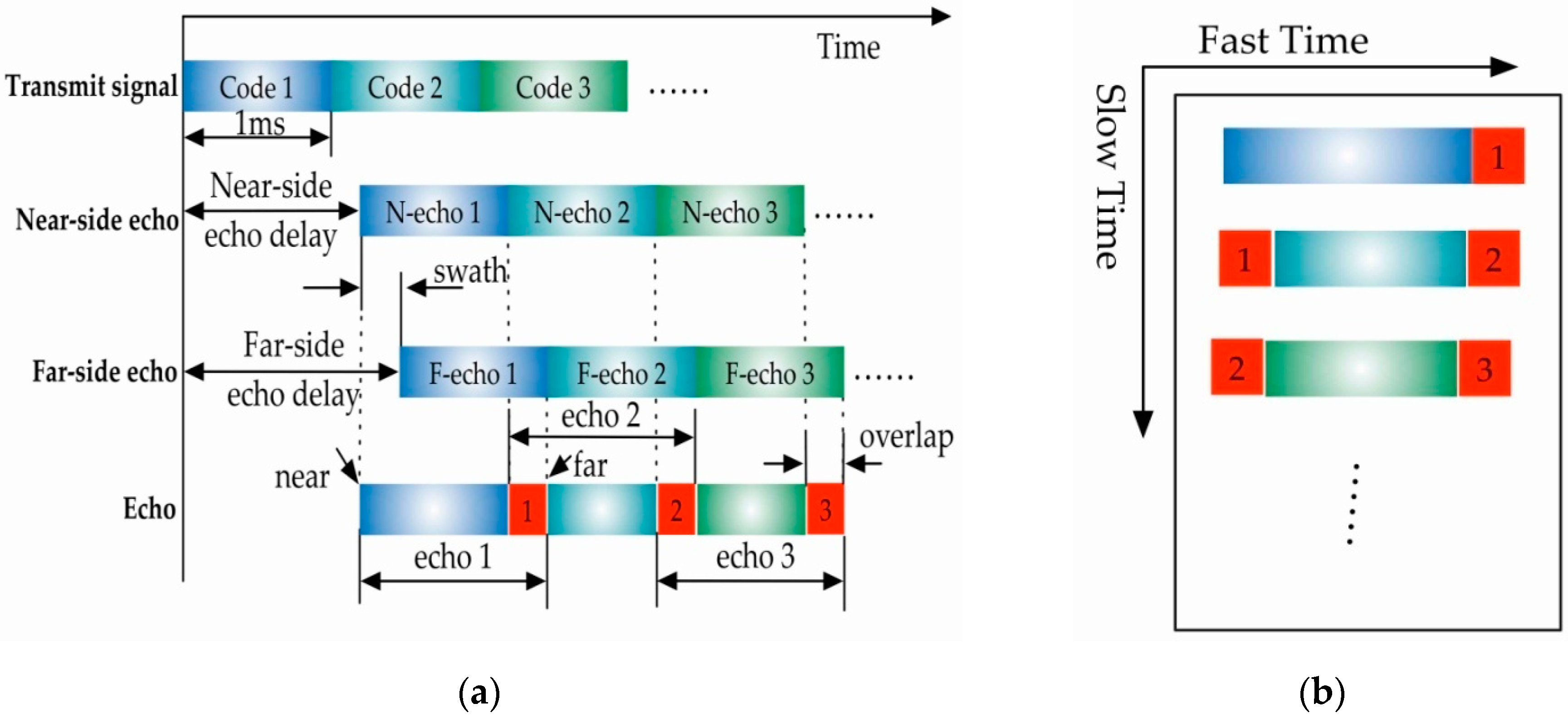
2. Signal Model of GNSS-Based Bistatic SAR
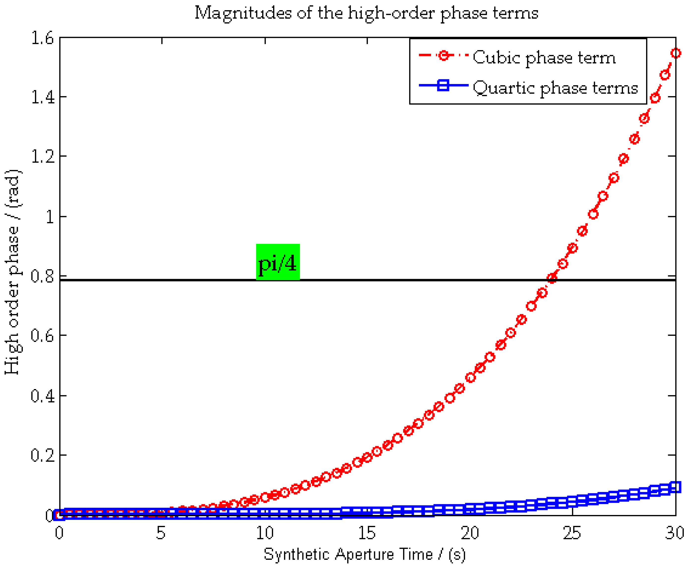
3. GNSS-Based Bistatic SAR Signal Analysis
3.1. 2-D Point Target Spectrum
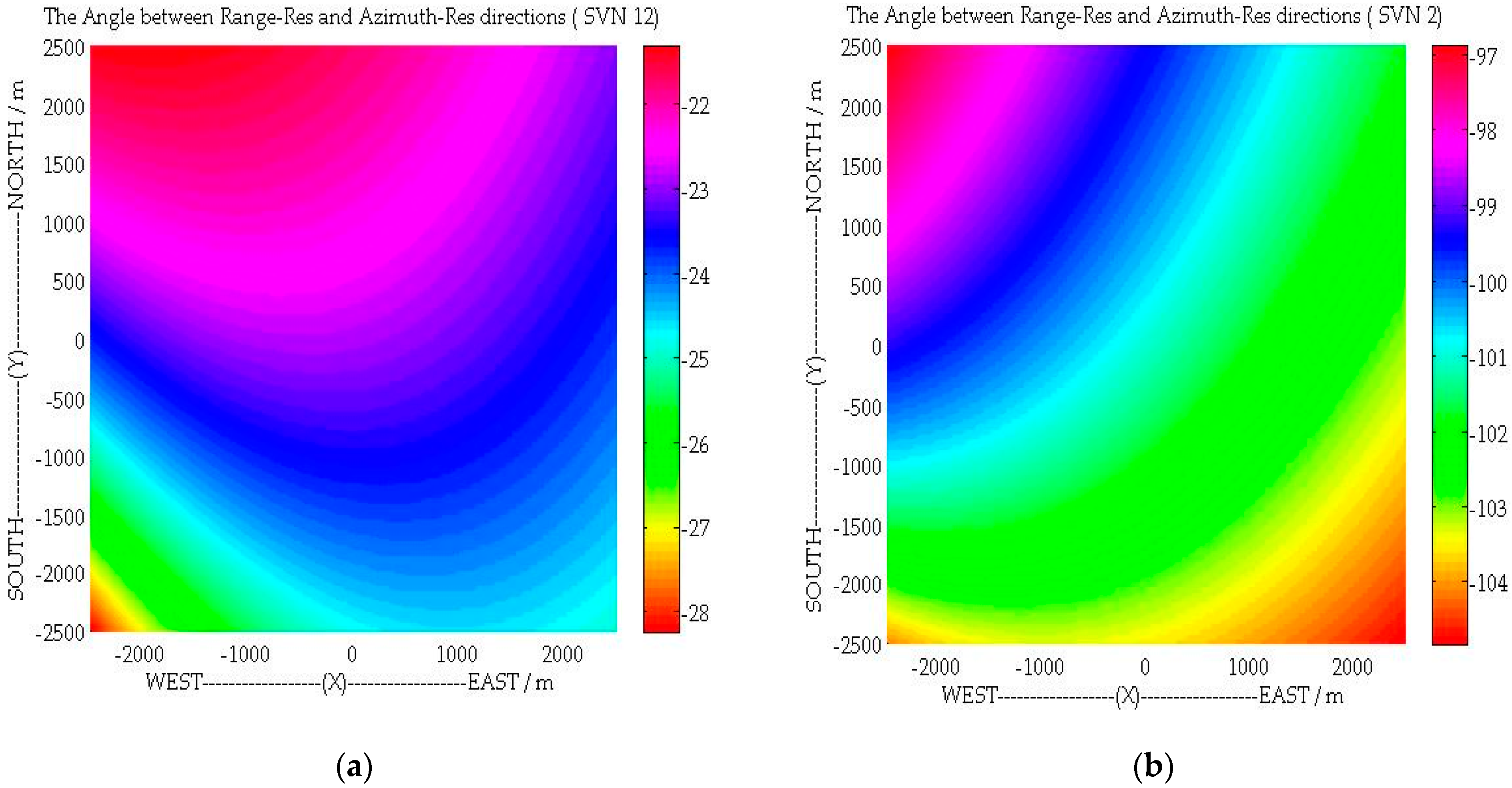
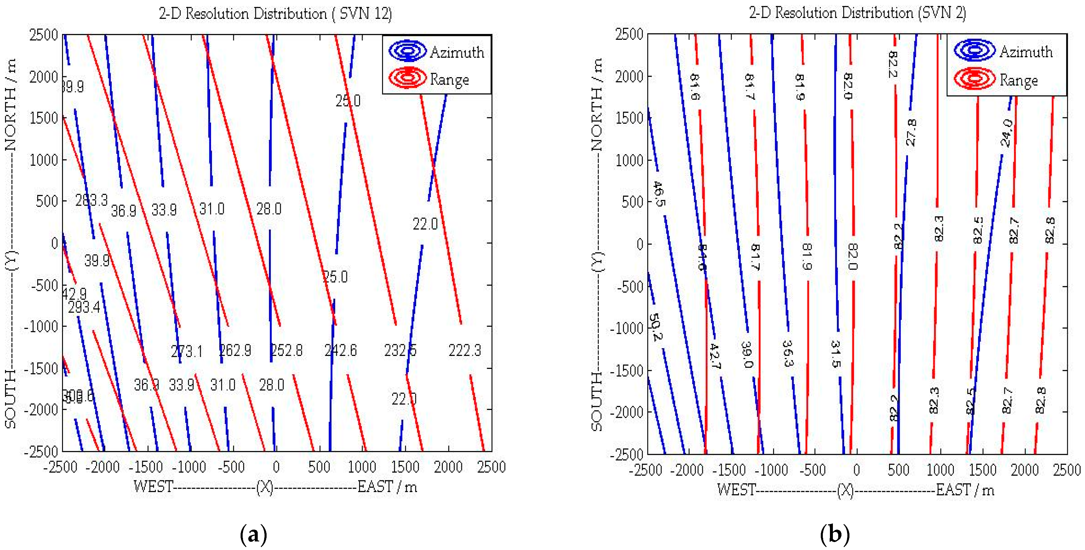
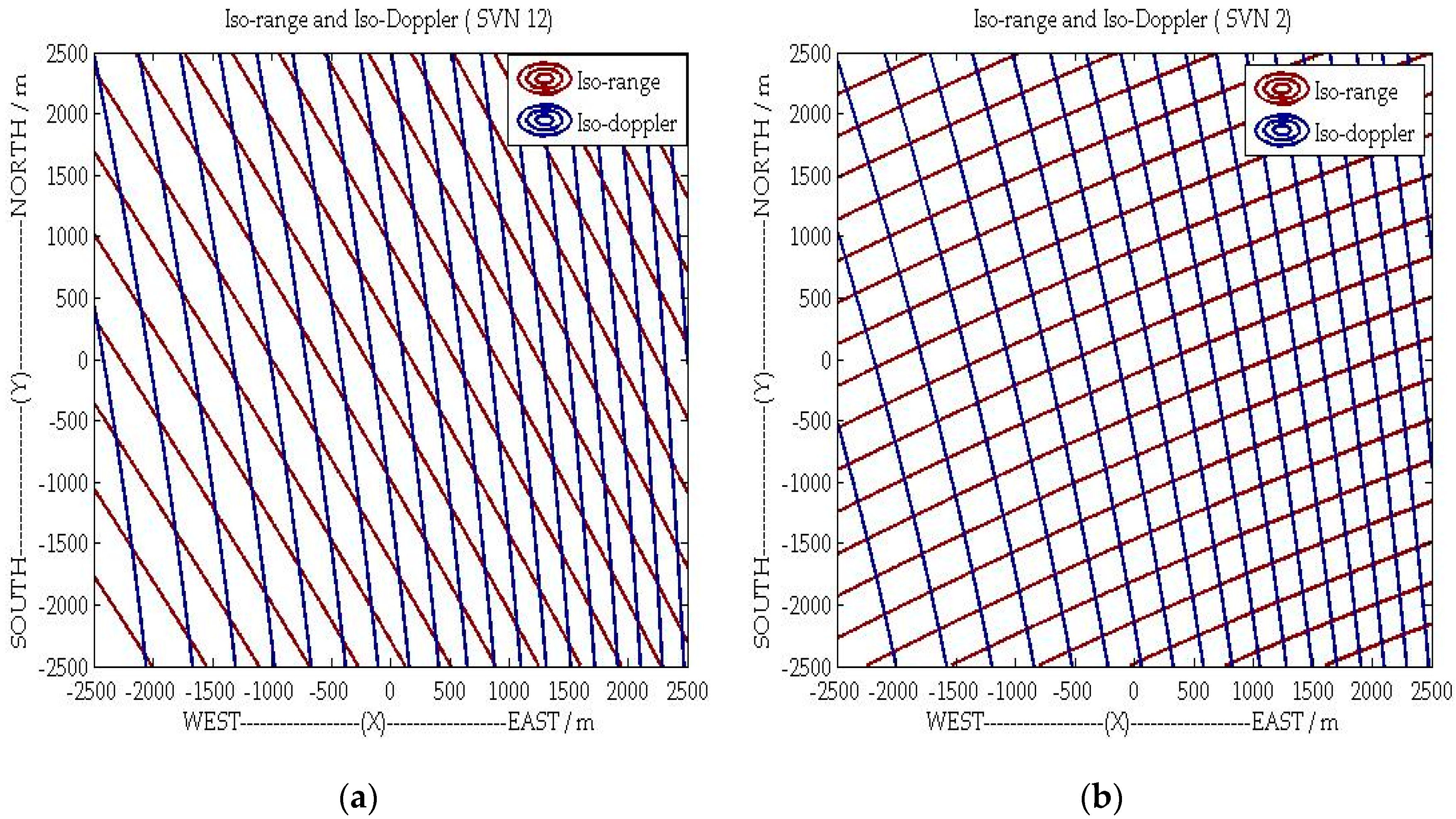
3.2. System Resolution of GNSS-Based Bistatic SAR
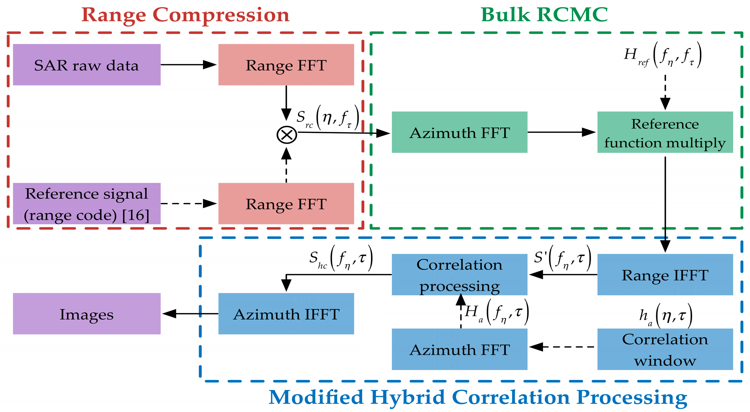
4. A General Imaging Algorithm
4.1. Range Compression
4.2. Bulk RCMC
4.3. Modified Hybrid Correlation Processing
5. Simulation and Discussions
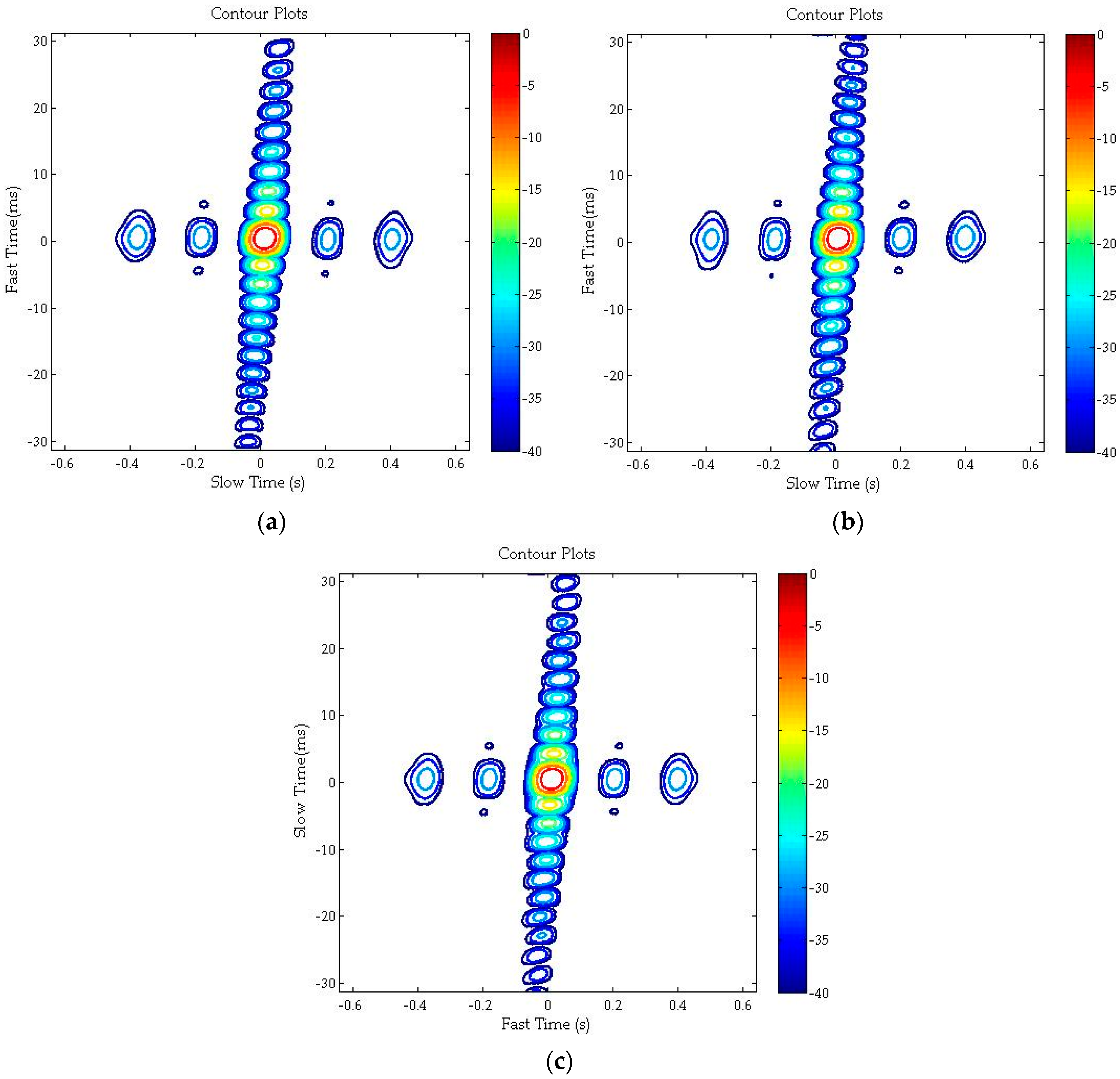
5.1. Comparative Experiments and Analysis
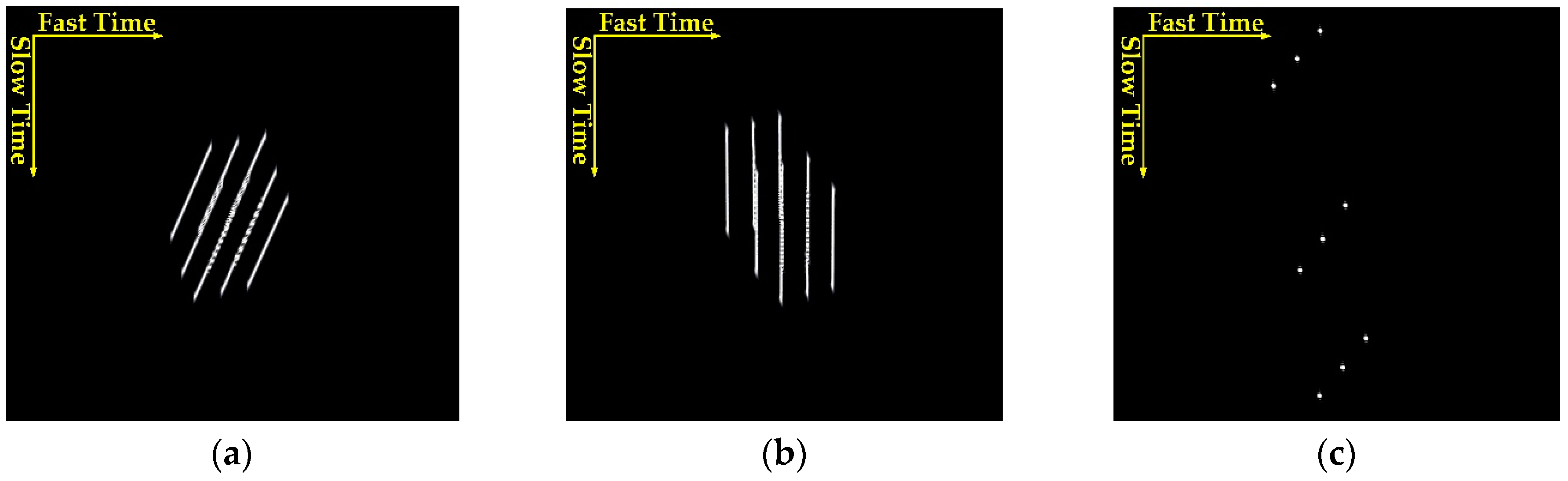
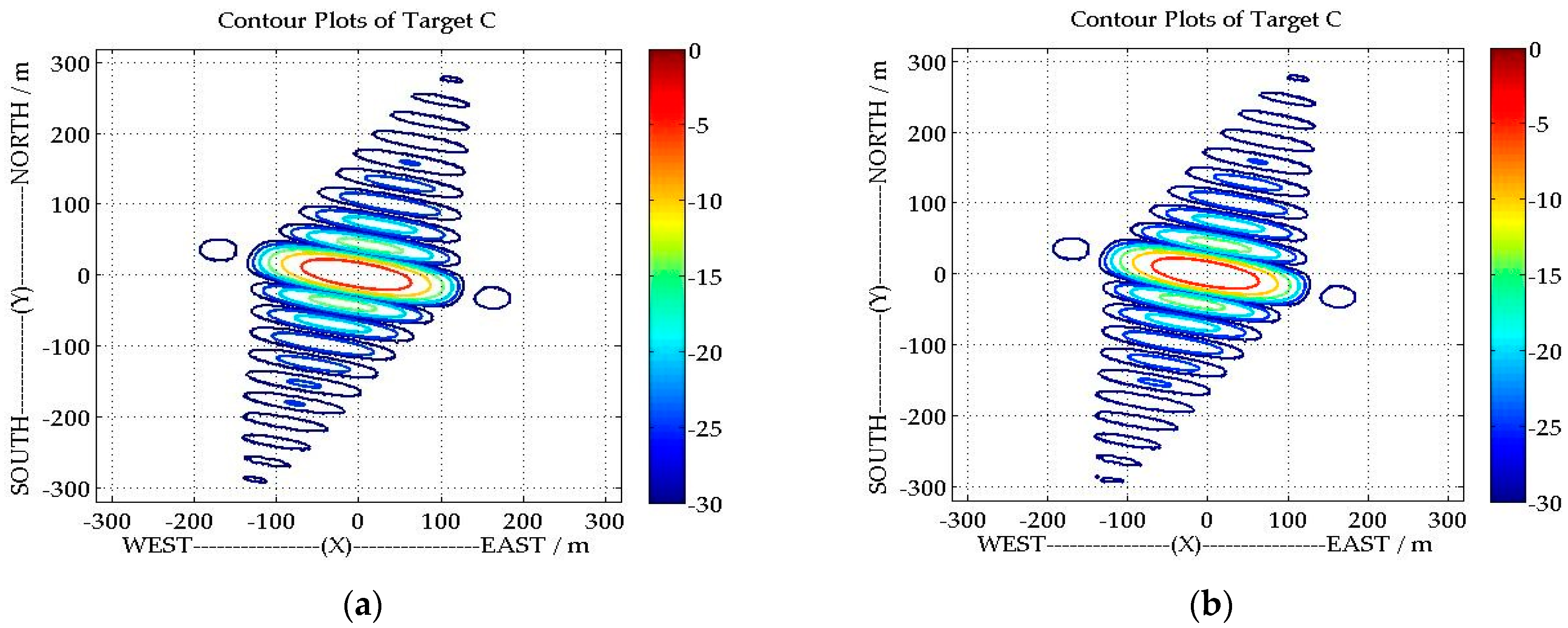
5.2. Imaging Simulation Experiments and Analysis
6. Conclusions
Acknowledgments
Author Contributions
Conflicts of Interest
References
- Moreira, A.; Krieger, G.; Hajnsek, I.; Papathanassiou, K.; Younis, M.; Lopez-Dekker, P.; Huber, S.; Villano, M.; Pardini, M.; Eineder, M.; et al. Tandem-L: A Highly Innovative Bistatic SAR Mission for Global Observation of Dynamic Processes on the Earth's Surface. IEEE Geosci. Remote Sens. Mag. 2015, 3, 8–23. [Google Scholar] [CrossRef]
- Walterscheid, I.; Espeter, T.; Brenner, A.R.; Klare, J.; Ender, J.H.G.; Nies, H.; Wang, R.; Loffeld, O. Bistatic SAR Experiments with PAMIR and TerraSAR-X--Setup, Processing and Image Results. IEEE Trans. Geosci. Remote Sens. 2010, 48, 3268–3279. [Google Scholar] [CrossRef]
- Rodriguez-Cassola, M.; Baumgartner, S.V.; Krieger, G.; Moreira, A. Bistatic TerraSR-X/F-SAR Spaceborne—Airborne SAR Experiment: Description, Data Processing and Results. IEEE Trans. Geosci. Remote Sens. 2010, 48, 781–794. [Google Scholar] [CrossRef]
- Gromek, D.; Samczynski, P.; Kulpa, K.; Krysik, P.; Malanowski, M. Initial results of passive SAR imaging using a DVB-T based on airborne radar receiver. In Proceedings of the 2014 11th European Radar Conference (EuRAD), Rome, Italy, 8–10 October 2014; pp. 137–140.
- Evers, A.; Jackson, J.A. Experimental passive SAR imaging exploiting LTE, DVB and DAB signals. In Proceedings of the 2014 IEEE Radar Conference, Cincinnati, OH, USA, 19–23 May 2014; pp. 680–685.
- Gutierrez Del Arroyo, J.R.; Jackson, J.A. WiMAX OFDM for Passive SAR Ground Imaging. IEEE Trans. Aerosp. Electron. Syst. 2013, 49, 945–959. [Google Scholar] [CrossRef]
- He, X.; Cherniakov, M.; Zeng, T. Signal detectability in SS-BSAR with GNSS non-cooperative transmitter. IEE Proc.-Radar, Sonar Navig. 2005, 152, 124–132. [Google Scholar] [CrossRef]
- Antoniou, M.; Zeng, Z.; Feifeng, L.; Cherniakov, M. Experimental demonstration of passive BSAR imaging using navigation satellites and a fixed receiver. IEEE Geosci. Remote Sens. Lett. 2012, 9, 477–481. [Google Scholar] [CrossRef]
- Jin, S.; Cardellach, E.; Xie, F. GNSS Remote Sensing: Theory, Methods and Applications; Springer: New York, NY, USA, 2014. [Google Scholar]
- Cherniakov, M. Bistatic Radar: Emerging technology, Chapter 9: Passive Bistatic SAR with GNSS Transimitters; Wiley: New York, NY, USA, 2008. [Google Scholar]
- Zavorotny, V.U.; Gleason, S.; Cardellach, E.; Camps, A. Tutorial on Remote Sensing Using GNSS Bistatic Radar of Opportunity. IEEE Geosci. Remote Sens. Mag. 2014, 2, 8–45. [Google Scholar] [CrossRef]
- Santi, F.; Antoniou, M.; Pastina, D. Point Spread Function analysis for GNSS-Based Multistatic SAR. IEEE Geosci. Remote Sens. Lett. 2015, 12, 304–308. [Google Scholar] [CrossRef]
- Zeng, T.; Ao, D.; Hu, C.; Zhang, T.; Liu, F.; Tian, W.; Lin, K. Multiangle BSAR imaging based on BeiDou-2 navigation satellites: Experiments and preliminary results. IEEE Trans. Geosci. Remote Sens. 2015, 53, 5760–5773. [Google Scholar] [CrossRef]
- Santi, F.; Bucciarelli, M.; Pastina, D.; Antoniou, M.; Tzagkas, D.; Cherniakov, M. Passive multistatic SAR with GNSS transmitters: Preliminary experimental study. In Proceedings of the 2014 11th European Radar Conference (EuRAD), Rome, Italy, 8–10 October 2014; pp. 129–132.
- Santi, F.; Bucciarelli, M.; Pastina, D.; Antoniou, M. CLEAN technique for passive bistatic and multistatic SAR with GNSS transmitters. In Proceedings of the 2015 IEEE Radar Conference (RadarCon), Arlington, VA, USA, 10–15 May 2015; pp. 1228–1233.
- Antoniou, M.; Cherniakov, M. GNSS-based bistatic SAR: A signal processing view. EURASIP J. Adv. Signal Process. 2013, 1, 1–16. [Google Scholar] [CrossRef]
- Tian, W.; Zhan, T.; Zeng, T.; Hu, C.; Long, T. Space-surface BiSAR based on GNSS signal: Synchronization, imaging and experiment result. In Proceedings of the 2014 IEEE Radar conference, Cincinnati, OH, USA, 19–23 May 2014; pp. 512–516.
- Neo, Y.L.; Wong, F.H.; Cumming, I.G. Processing of azimuth-invariant bistatic SAR data using the range Doppler algorithm. IEEE Trans. Geosci. Remote Sens. 2008, 46, 14–21. [Google Scholar] [CrossRef]
- Qiu, X.; Hu, D.; Ding, C. An omega-K algorithm with phase error compensation for bistatic SAR of a translational invariant case. IEEE Trans. Geosci. Remote Sens. 2008, 46, 2224–2232. [Google Scholar]
- Zeng, D.; Zeng, T.; Hu, C.; Long, T. Back-projection algorithm characteristic analysis in forward-looking bistatic SAR. In Proceedings of the International Conference on Radar (CIE’06), Shanghai, China, 16–19 October 2006; pp. 1–4.
- Wong, F.H.; Cumming, I.G.; Neo, Y.L. Focusing bistatic SAR data using the non-linear chirp scaling algorithm. IEEE Trans. Geosci. Remote Sens. 2008, 46, 2493–2505. [Google Scholar] [CrossRef]
- Liu, H.W.; Wang, T.; Wu, Q.; Bao, Z. Bistatic SAR Data Focusing Using an Omega-k Algorithm based on Method of Series Reversion. IEEE Trans. Geosci. Remote Sens. 2009, 47, 2899–2912. [Google Scholar]
- Antoniou, M.; Saini, R.; Cherniakov, M. Results of a Space-surface Bistatic SAR Image Formation Algorithm. IEEE Trans. Geosci. Remote Sens. 2007, 45, 3359–3371. [Google Scholar] [CrossRef]
- Wu, C.; Liu, K.; Jin, M. Modeling and a correlation algorithm for spaceborne SAR signals. IEEE Trans. Aerosp. Electron. Syst. 1982, 18, 563–575. [Google Scholar] [CrossRef]
- Wang, P.; Liu, W.; Chen, J.; Niu, M.; Yang, W. A High-Order Imaging Algorithm for High-Resolution Spaceborne SAR Based on a Modified Equivalent Squint Range Model. IEEE Trans. Geosci. Remote Sens. 2015, 53, 1225–1235. [Google Scholar] [CrossRef]
- Ortiz, A.M.; Loffeld, O.; Wang, R.; Nies, H. Motion Compensation in Bistatic SAR for Hybrid Experiment. In Proceedings of the 2008 7th European Conference on Synthetic Aperture Radar (EUSAR), Friedrichshafen, Germany, 2–5 June 2008; pp. 1–4.
- Nies, H.; Loffeld, O.; Natroshvili, K.; Ortiz, A.M. A Solution for Bistatic Motion Compensation. In Proceedings of the IEEE International Conference on Geoscience and Remote Sensing Symposium (IGARSS 2006), Denver, CO, USA, 31 July–4 August 2006; pp. 204–1207.
- Saini, R.; Zuo, R.; Cherniakov, M. Problem of signal synchronization in space-surface bistatic synthetic aperture radar based on global navigation satellite emissions experimental results. IET Proc. Radar Sonar Navigat. 2010, 4, 110–125. [Google Scholar] [CrossRef]
- Cumming, I.; Wong, F. Digital Processing of Synthetic Aperture Radar Data: Algorithms and Implementation; Artech House: Norwood, MA, USA, 2005. [Google Scholar]
- Neo, Y.L.; Wong, F.; Cumming, I.G. A two-dimensional spectrum for bistatic SAR processing using series reversion. IEEE Geosci. Remote Sens. Lett. 2007, 4, 93–96. [Google Scholar] [CrossRef]
- Antonio, M.; Alfredo, R. Spatial Resolution of Bistatic Synthetic Aperture Radar: Impact of Acquisition Geometry on Imaging Performance. IEEE Trans. Geosci. Remote Sens. 2011, 49, 3487–3503. [Google Scholar]
- Zeng, T.; Cherniakov, M.; Long, T. Generalized approach to resolution analysis in BSAR. IEEE Trans. Aerosp. Electron Syst. 2005, 41, 461–474. [Google Scholar] [CrossRef]
- Cardillo, G.P. On the use of the gradient to determine bistatic SAR resolution. Antennas Propag. Soc. Int. Symp. 1990, 2, 1032–1035. [Google Scholar]
- Misra, P.; Enge, P. GPS Signals, Measurements, and Performance; Ganga-Jamuna Press: Lincoln, MA, USA, 2006. [Google Scholar]
- Hui, M.; Antoniou, M.; Cherniakov, M. Passive GNSS-based SAR Resolution Improvement Using Joint Galileo E5 Signals. IEEE Geosci. Remote Sens. Lett. 2015, 12, 1640–1644. [Google Scholar] [CrossRef]


| Parameters | Value |
|---|---|
| Receiver center position | (6, −25,5) km |
| Receiver velocity | (−30, 60, 0) m/s |
| Transmitter center position (SVN 2) | (1.0235, −1.5541, 1.2402) × 104 km |
| Transmitter center position (SVN 12) | (−1.8028, 1.6145, 0.4677) × 104 km |
| Transmitter center velocity (SVN 2) | (185.6, −2113.7, −1800.0) m/s |
| Transmitter center velocity (SVN 12) | (−2096.1, −730.7, −2321.8) m/s |
| Synthetic aperture time | 10.0 s |
| Signal bandwidth (GPS C/A) | 2.046 MHz |
| Signal wavelength | 0.19 m |
| Sampling rate | 5.0 MHz |
| PRF | 100 Hz |
| Azimuth | Range | |||||
|---|---|---|---|---|---|---|
| Traditional BPA | 30.08 | −13.30 | −10.22 | 82.05 | −27.34 | −19.43 |
| Proposed Algorithm | 30.08 | −13.30 | −10.23 | 82.05 | −27.34 | −19.42 |
| Azimuth | Range | |||||||
|---|---|---|---|---|---|---|---|---|
| ρa,m (m) | Widen Ratio | PSLR (dB) | ISLR (dB) | ρr,m (m) | Widen Ratio | PSLR (dB) | ISLR (dB) | |
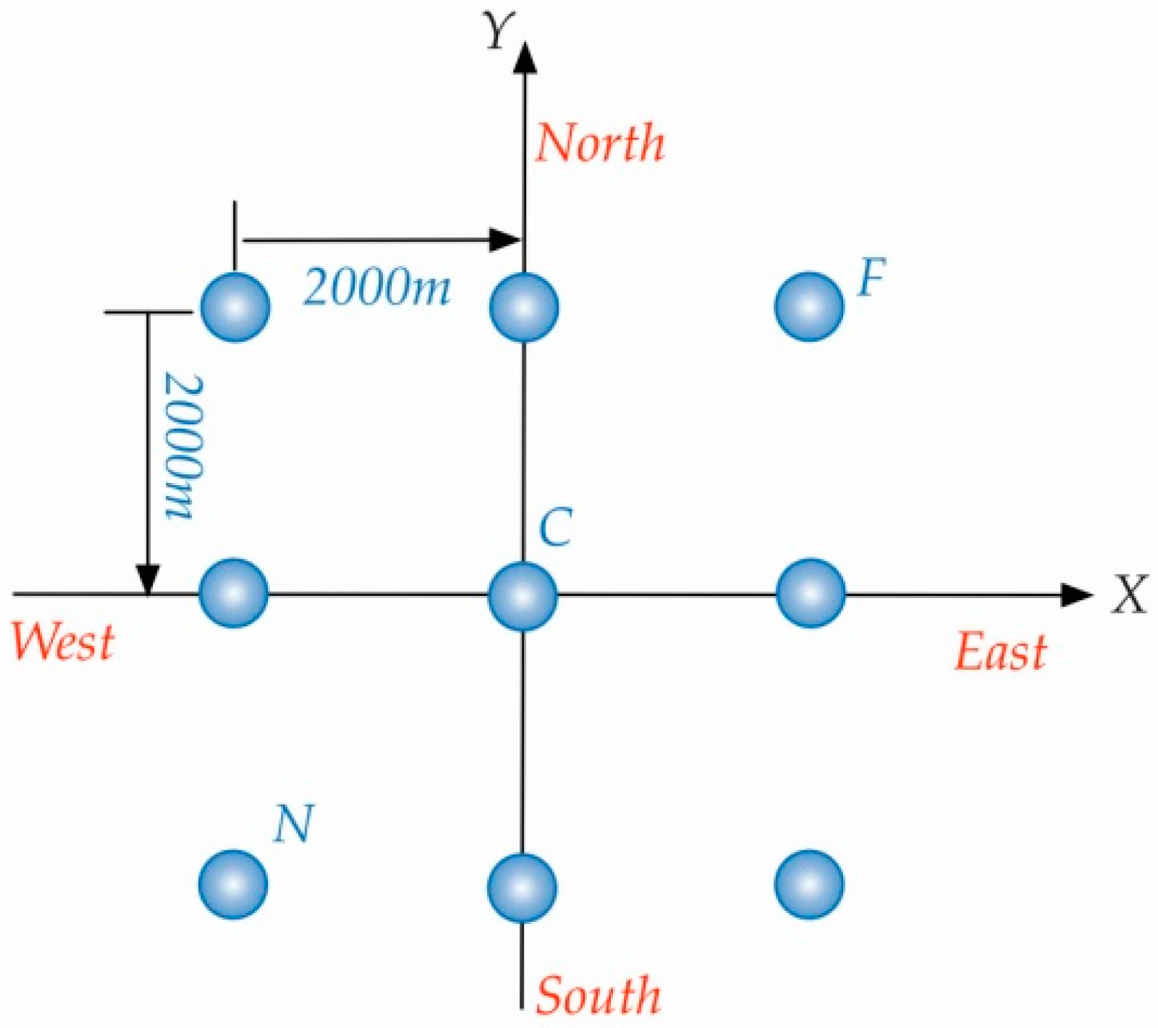
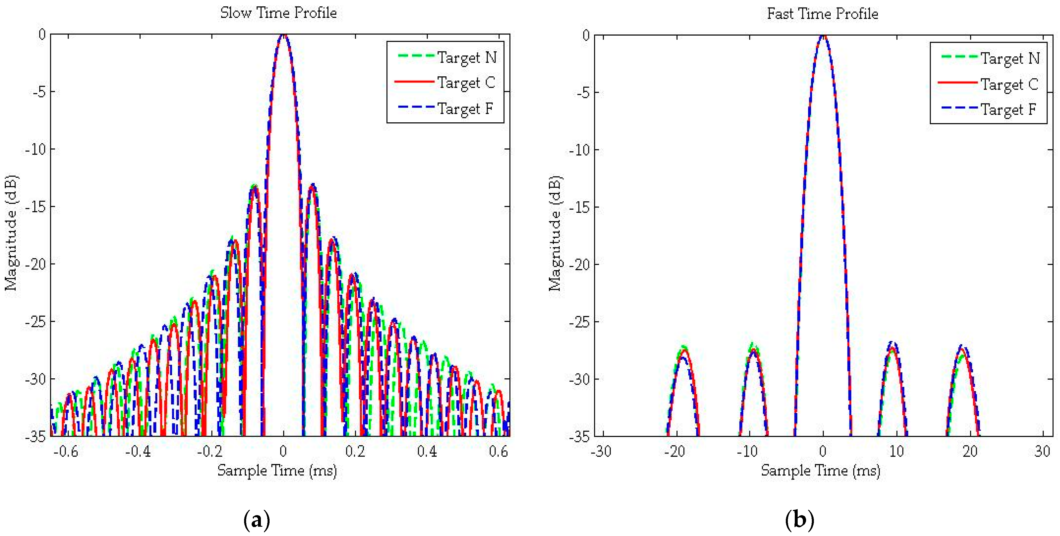
| N | 48.16 | 1.032 | −13.26 | −10.20 | 81.54 | 1.012 | −27.09 | −19.40 |
| C | 30.08 | 1.029 | −13.30 | −10.23 | 82.05 | 1.011 | −27.34 | −19.42 |
| F | 23.61 | 1.031 | −13.24 | −10.19 | 82.68 | 1.014 | −26.99 | −19.37 |
© 2016 by the authors; licensee MDPI, Basel, Switzerland. This article is an open access article distributed under the terms and conditions of the Creative Commons by Attribution (CC-BY) license (http://creativecommons.org/licenses/by/4.0/).
Share and Cite
Zeng, H.-C.; Wang, P.-B.; Chen, J.; Liu, W.; Ge, L.; Yang, W. A Novel General Imaging Formation Algorithm for GNSS-Based Bistatic SAR. Sensors 2016, 16, 294. https://doi.org/10.3390/s16030294
Zeng H-C, Wang P-B, Chen J, Liu W, Ge L, Yang W. A Novel General Imaging Formation Algorithm for GNSS-Based Bistatic SAR. Sensors. 2016; 16(3):294. https://doi.org/10.3390/s16030294
Chicago/Turabian StyleZeng, Hong-Cheng, Peng-Bo Wang, Jie Chen, Wei Liu, LinLin Ge, and Wei Yang. 2016. "A Novel General Imaging Formation Algorithm for GNSS-Based Bistatic SAR" Sensors 16, no. 3: 294. https://doi.org/10.3390/s16030294
APA StyleZeng, H.-C., Wang, P.-B., Chen, J., Liu, W., Ge, L., & Yang, W. (2016). A Novel General Imaging Formation Algorithm for GNSS-Based Bistatic SAR. Sensors, 16(3), 294. https://doi.org/10.3390/s16030294